
Mathematics Optional · UPSC Notes
Calculus — UPSC Maths Optional Notes
Free, exam-focused notes for UPSC Prelims and Mains, with Prelims tips and Mains points for every topic. 9 topics.
Open in the interactive reader: bookmarks, progress tracking and read-aloud.
Real Numbers, Limits, Continuity and Differentiability
ℝ is a complete ordered field: every non-empty set bounded above has a supremum. Limits are defined by ε-δ, and f is continuous at a when limx→a f(x) = f(a). Differentiability implies continuity but not conversely, and a continuous function on a closed bounded interval is bounded, attains its bounds and is uniformly continuous.
1. Understanding the Supremum and Completeness
Why we need it: calculus keeps producing points: the point where a continuous curve crosses a level, the highest point of a graph, the point where a tangent is horizontal.
We need a guarantee that such a point really exists as a number. On the rational numbers ℚ alone this guarantee fails, so we need an axiom that says the real line has no holes.
In words: a number M is an upper bound of a set S if no element of S is bigger than M.
A set can have many upper bounds; if 5 is one, so are 6 and 100. The supremum (least upper bound) is the smallest of them.
'M = sup S' therefore has two parts. Part 1: x ≤ M for every x ∈ S (M is a ceiling). Part 2: for every ε > 0 some x ∈ S satisfies x > M − ε (no lower ceiling works).
Read the quantifiers carefully: 'for every ε' comes first, and the element x may depend on ε. The infimum is defined the same way with the inequalities reversed.
The completeness axiom says: every non-empty set of reals that has some upper bound has a supremum that is itself a real number.
First example, slowly: take S = {1 − 1/n : n ∈ ℕ} = {0, 1/2, 2/3, 3/4, ...}.
Step 1 (guess): the elements increase towards 1, so guess sup S = 1.
Step 2 (ceiling): 1 − 1/n < 1 for every n, because 1/n > 0. So 1 is an upper bound.
Step 3 (no lower ceiling): let ε > 0. By the Archimedean property choose n with n > 1/ε. Then 1/n < ε, so 1 − 1/n > 1 − ε.
Step 4 (conclude): both parts hold, so sup S = 1. Notice that 1 ∉ S: a supremum need not be an element of the set. Here inf S = min S = 0, which is attained at n = 1.
Non-example: inside ℚ, the set A = {x ∈ ℚ : x > 0, x2 < 2} is bounded above (by 2) but has no least rational upper bound.
Any rational upper bound r has r2 > 2 (no rational squares to 2), and then a slightly smaller rational is still an upper bound. The condition that fails is completeness: the 'supremum' √2 is missing from ℚ.
Building up: completeness is the engine behind the big theorems on [a, b].
For the intermediate value theorem one takes c = sup{x ∈ [a, b] : f(x) < k} and shows f(c) = k (Standard Proofs, Theorem 2).
Completeness also gives the Bolzano-Weierstrass theorem (every bounded sequence has a convergent subsequence), which proves boundedness, attainment of bounds and uniform continuity (Theorems 3, 4 and 10).
Where it is used: UPSC asks for sup and inf of sets such as {1/m + 1/n} or {(−1)n/n}: always prove both parts, and say whether the bound is attained.
In Real Analysis the same idea gives the monotone convergence theorem and Cauchy's criterion for sequences.
2. Real Number System
ℝ is a complete ordered field. Completeness (LUB) axiom: every non-empty subset of ℝ that is bounded above has a least upper bound (supremum) in ℝ.
Idea: completeness says the real line has no gaps: every set that is bounded above has a least 'ceiling', and that ceiling is itself a real number. ℚ has gaps (at √2, π, ...), and every theorem below that produces a point (intermediate value theorem, extreme values, Rolle) depends on completeness: x2 − 2 changes sign on [1, 2] ∩ ℚ but has no rational zero.
Archimedean property: for any x, y > 0 there is n ∈ ℕ with nx > y. Between any two real numbers there lie both a rational and an irrational number (density).
Derivation (a rational between x < y): by the Archimedean property choose n ∈ ℕ with n(y − x) > 1, and let m be the least integer greater than nx. Then m − 1 ≤ nx < m, so nx < m ≤ nx + 1 < ny, that is x < m/n < y.
For an irrational, take a rational r with x − √2 < r < y − √2; then r + √2 is irrational and lies between x and y.
sup S = M means: x ≤ M for all x ∈ S, and for every ε > 0 there is x ∈ S with x > M − ε. ℚ is not complete: {x ∈ ℚ: x2 < 2} has no supremum in ℚ.
Idea: M is an upper bound that cannot be lowered, since any smaller number M − ε is beaten by some element of S. The supremum need not belong to S: sup{1 − 1/n: n ∈ ℕ} = 1, which is not in the set.
3. Understanding the ε-δ Definition of a Limit
Why we need it: 'f(x) gets close to l as x gets close to a' is too vague to prove anything. How close, and close for which x?
The ε-δ definition turns 'close' into two numbers, so that a limit can be proved or disproved by inequalities.
In words: limx→a f(x) = l means: for every ε > 0 there is δ > 0 such that 0 < |x − a| < δ implies |f(x) − l| < ε.
ε is the output tolerance: how far f(x) may be from l. It is given to you, and it may be as small as the opponent likes.
δ is the input window: how near x must be to a. You must find it, and it may depend on ε.
'0 < |x − a|' excludes x = a itself, so the value f(a) never matters for the limit.
First example, slowly: prove limx→1 (3x + 2) = 5.
Step 1 (work backwards): we want |(3x + 2) − 5| < ε. Simplify: |3x − 3| = 3|x − 1|.
Step 2: 3|x − 1| < ε holds exactly when |x − 1| < ε/3. So choose δ = ε/3.
Step 3 (write forwards): given ε > 0, let δ = ε/3. If 0 < |x − 1| < δ, then |(3x + 2) − 5| = 3|x − 1| < 3δ = ε.
Step 4: notice that δ depends on ε (smaller ε, smaller δ), which is allowed. For a non-linear f, first restrict to |x − a| < 1 to bound the extra factor, as in the method below.
Non-example: f(x) = sin(1/x) has no limit as x → 0.
Along xn = 1/(2nπ + π/2), f = 1; along yn = 1/(2nπ), f = 0; both sequences tend to 0.
Whatever l you propose, with ε = 1/2 every window around 0 contains points where f = 1 and points where f = 0, and these cannot both be within 1/2 of l. The condition 'there is δ' fails.
Building up: from the definition one proves the algebra of limits (sum, product, quotient with non-zero limit), the squeeze theorem and the sequential criterion.
For the squeeze theorem: if g ≤ f ≤ h near a and g, h → l, take the smaller of the two δ's for g and h; then l − ε < g ≤ f ≤ h < l + ε.
The sequential criterion converts every limit question into one about sequences: a single bad sequence disproves a limit, but a proof needs all sequences (or a direct ε-δ argument).
Where it is used: 'find δ for a given ε' questions (often with ε = 0.01), limits of functions of two variables, and every definition that follows: continuity, derivative, Riemann integral.
4. Limits
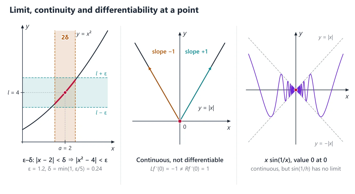
limx→a f(x) = l if for every ε > 0 there is δ > 0 such that 0 < |x − a| < δ ⇒ |f(x) − l| < ε.
Idea: read the definition as a challenge: for every tolerance ε demanded around l, one can find a window of half-width δ around a (excluding a itself) on which f stays within that tolerance. The value f(a), and even whether f is defined at a, plays no part.
Finding δ (method): factor |f(x) − l| as |x − a|·g(x), bound g by a constant K on |x − a| < 1, and take δ = min(1, ε/K). For x2 → 4 as x → 2: |x2 − 4| = |x − 2||x + 2| ≤ 5|x − 2| when |x − 2| < 1, so δ = min(1, ε/5) works.
The limit exists if and only if the left limit f(a − 0) and the right limit f(a + 0) exist and are equal.
Sequential criterion: limx→a f(x) = l if and only if f(xn) → l for every sequence xn → a with xn ≠ a; to show that a limit does not exist, find two such sequences along which f has different limits.
Standard limits: limx→0 (sin x)/x = 1, limx→0 (ex − 1)/x = 1, limx→0 (1 + x)1/x = e, limx→0 (ax − 1)/x = log a (a > 0).
Derivation of lim (sin x)/x = 1: for 0 < x < π/2, comparing the areas of the triangle, the sector and the tangent triangle on an arc x of the unit circle gives sin x < x < tan x, so cos x < (sin x)/x < 1. Since cos x → 1 and (sin x)/x is even, the squeeze (sandwich) theorem gives the limit 1; the angle must be in radians.
5. Understanding Continuity and Uniform Continuity
Why we need it: we want functions whose values can be predicted from nearby values: a small error in x should cause only a small error in f(x).
Continuity is exactly this property at one point; uniform continuity asks for it with the same precision across the whole interval.
In words: f is continuous at a when three things hold: f(a) is defined, limx→a f(x) exists, and the two are equal.
In ε-δ language: for every ε > 0 there is δ > 0 with |x − a| < δ ⇒ |f(x) − f(a)| < ε. Here x = a is allowed, since f(a) is now the target.
For uniform continuity on a set I, the order of the quantifiers changes: δ is chosen after ε but before the points, so one δ works for every pair x, y ∈ I with |x − y| < δ.
First example, slowly: test f(x) = (x2 − 4)/(x − 2) for x ≠ 2, f(2) = 3, at x = 2.
Step 1: f(2) = 3 is defined.
Step 2: for x ≠ 2, f(x) = (x − 2)(x + 2)/(x − 2) = x + 2, so limx→2 f(x) = 4. Cancelling is legal because the limit never uses x = 2.
Step 3: 4 ≠ 3, so f is discontinuous at 2. The limit exists, so the discontinuity is removable: redefining f(2) = 4 makes f continuous.
Step 4 (uniformity): on all of ℝ the redefined f(x) = x + 2 satisfies |f(x) − f(y)| = |x − y|, so δ = ε works at every point at once: f is uniformly continuous.
Non-example: f(x) = x2 is continuous at every point of ℝ but not uniformly continuous on ℝ.
Take xn = n + 1/n and yn = n. Then |xn − yn| = 1/n → 0, but xn2 − yn2 = 2 + 1/n2 > 2.
So for ε = 2 no single δ works: the graph gets steeper as x grows, and the δ needed at x shrinks like ε/(2|x|). The failing condition is 'δ independent of the point'.
Building up: continuity is preserved by sums, products, quotients (non-zero denominator) and composition, because limits are.
On a closed bounded interval continuity becomes much stronger: f is bounded, attains its maximum and minimum, takes every intermediate value and is uniformly continuous (Standard Proofs, Theorems 2, 3, 4 and 10).
The proof of uniform continuity (Heine-Cantor) argues by contradiction: if one ε defeats every δ = 1/n, Bolzano-Weierstrass gives a limit point c where continuity fails, which is impossible.
Where it is used: classifying discontinuities of piecewise functions, finding the constant that makes f continuous, IVT root-existence questions, and proving Riemann integrability of continuous functions.
6. Continuity
f is continuous at a if limx→a f(x) = f(a), that is, f(a − 0) = f(a + 0) = f(a).
Idea: continuity means no jump, no hole and no wild oscillation at a, so the graph can be drawn near a without lifting the pen. Equivalently (sequential form), xn → a implies f(xn) → f(a).
Discontinuities: removable (the limit exists but differs from f(a), or f(a) is undefined); first kind or jump (both one-sided limits exist but differ); second kind (at least one one-sided limit does not exist, for example sin(1/x) at 0).
Theorems on [a, b]: a function continuous on a closed bounded interval is bounded, attains its supremum and infimum, takes every value between f(a) and f(b) (intermediate value theorem), and is uniformly continuous.
These are proved in Standard Proofs, Theorems 2, 3, 4 and 10. Both 'closed' and 'bounded' are needed: 1/x on (0, 1] is continuous but unbounded, x on (0, 1) has no maximum, and x/(1 + x) on [0, ∞) is bounded but never attains its supremum 1.
Uniform continuity: for every ε > 0 there is δ > 0, independent of the point, with |x − y| < δ ⇒ |f(x) − f(y)| < ε. Example: 1/x is continuous but not uniformly continuous on (0, 1), and x2 is not uniformly continuous on ℝ.
Idea: one δ must serve every point at once. The graph of 1/x gets steeper and steeper near 0, so the δ that works at x shrinks to 0 as x → 0+. A bounded derivative, |f′| ≤ K, gives uniform continuity with δ = ε/K, since |f(x) − f(y)| = |f′(c)||x − y| ≤ K|x − y| by the MVT.
Exponential one-sided limits: as x → 0+, e1/x → ∞ and e−1/x → 0; as x → 0−, e1/x → 0 and e−1/x → ∞. Functions built from e±1/x usually have a jump at 0, so always compute both one-sided limits.
Value that makes f continuous: if f is given by a formula on [a, b) and is to be continuous on [a, b], then f(b) must equal limx→b− f(x), which is often a 0/0 form.
7. Understanding the Derivative
Why we need it: to measure how fast a quantity changes at one instant (speed, slope of a tangent, marginal cost) we need more than continuity.
The derivative turns 'rate of change at a point' into a limit that can be computed and tested.
In words: (f(a + h) − f(a))/h is the slope of the chord from (a, f(a)) to (a + h, f(a + h)).
f′(a) is the limit of these chord slopes as h → 0 from both sides. If h → 0+ only, we get the right derivative Rf′(a); if h → 0− only, the left derivative Lf′(a).
f is differentiable at a exactly when both one-sided derivatives exist, are finite and are equal.
First example, slowly: f(x) = x|x| at a = 0.
Step 1: f(0) = 0, so the difference quotient is (f(h) − 0)/h = h|h|/h = |h|.
Step 2: as h → 0+, |h| = h → 0, so Rf′(0) = 0. As h → 0−, |h| = −h → 0, so Lf′(0) = 0.
Step 3: both are finite and equal, so f′(0) = 0, although f is built from |x|, which has a corner at 0.
Step 4: away from 0, f(x) = x2 (x > 0) or −x2 (x < 0), so f′(x) = 2|x| for every x. This f′ is continuous but has a corner at 0, so f″(0) does not exist.
Non-example: f(x) = x1/3 at 0 is continuous, and its graph even has a tangent line there (the y-axis).
But (f(h) − f(0))/h = h−2/3 → +∞, so the limit is not finite and f is not differentiable at 0. The condition that fails is finiteness, not equality of the two sides.
Building up: writing f(a + h) − f(a) = h·(difference quotient) shows at once that a differentiable function is continuous (Standard Proofs, Theorem 1).
The same identity, with care at points where f(x) = f(a), gives the product, quotient and chain rules (derived below).
Darboux's theorem then shows that derivatives, even discontinuous ones, have the intermediate value property (Standard Proofs, Theorem 9).
Where it is used: differentiability at junction points of piecewise and modulus functions, functional equations, and as the hypothesis of Rolle, the mean value theorems and Taylor's theorem in the next topic.
8. Differentiability
f′(a) = limh→0 (f(a + h) − f(a))/h; f is differentiable at a if the left derivative Lf′(a) and the right derivative Rf′(a) are finite and equal.
Idea: f′(a) is the slope of the tangent, the limit of the slopes of chords through (a, f(a)). Differentiability means that f is approximately linear near a: f(a + h) = f(a) + hf′(a) + hε(h) with ε(h) → 0.
Differentiability ⇒ continuity, but not conversely: |x| is continuous at 0 with Lf′(0) = −1 and Rf′(0) = 1.
Proved in Standard Proofs, Theorem 1. Further standard examples (value 0 at x = 0): x sin(1/x) is continuous but not differentiable at 0; x2 sin(1/x) is differentiable at 0 with f′(0) = 0, but f′(x) = 2x sin(1/x) − cos(1/x) for x ≠ 0 has no limit at 0, so f′ is not continuous there.
Darboux's theorem: if f is differentiable on [a, b], then f′ takes every value between f′(a) and f′(b); hence a derivative cannot have a jump discontinuity.
Proved in Standard Proofs, Theorem 9. Idea: a derivative can be discontinuous, as for x2 sin(1/x), but only by oscillating, never by jumping; so a step function such as sgn x is not the derivative of any function on an interval containing 0.
Modulus functions: if g is differentiable at c, g(c) = 0 and g′(c) ≠ 0, then |g| has one-sided derivatives −|g′(c)| and |g′(c)| at c and is not differentiable there; where g(c) ≠ 0, |g| equals g or −g near c.
Derivative of a determinant: if the entries are differentiable functions of x, the derivative is the sum of the determinants obtained by differentiating one row at a time.
Functional equations: for f(x + y) = f(x)f(y) or f(x + y) = f(x) + f(y), put x = y = 0 to find f(0), then compute f′(x) from first principles using the equation. f′ = kf with f(0) = 1 gives f = ekx; f′ = k with f(0) = 0 gives f = kx.
9. Derivation: Product and Chain Rules from the Definition
Product rule: f(a + h)g(a + h) − f(a)g(a) = f(a + h)[g(a + h) − g(a)] + g(a)[f(a + h) − f(a)]. Divide by h and let h → 0; f(a + h) → f(a) because f is differentiable, hence continuous, at a, so (fg)′(a) = f(a)g′(a) + g(a)f′(a).
Carathéodory's form: f is differentiable at a if and only if f(x) − f(a) = φ(x)(x − a) for a function φ continuous at a, and then f′(a) = φ(a) (take φ(x) = (f(x) − f(a))/(x − a) for x ≠ a and φ(a) = f′(a)).
Chain rule: write f(x) − f(a) = φ(x)(x − a) and g(y) − g(f(a)) = ψ(y)(y − f(a)). Then g(f(x)) − g(f(a)) = ψ(f(x))φ(x)(x − a), and ψ(f(x))φ(x) is continuous at a with value g′(f(a))f′(a), so (g∘f)′(a) = g′(f(a))f′(a). This avoids the false step of dividing by f(x) − f(a), which may be 0 for x ≠ a.
10. Choosing the Method
If f is defined piecewise → at the junction compute f(a − 0), f(a + 0) and f(a) for continuity, and Lf′(a), Rf′(a) from the definition for differentiability; away from the junction the usual rules apply.
If you suspect that a limit does not exist → find two sequences xn, yn → a (both ≠ a) along which f has different limits; if you must prove a limit exists → use an ε-δ estimate, the squeeze theorem or standard limits, never a single sequence.
The table in this topic collects the standard situations; examiners expect the one-sided limits or derivatives to be written out explicitly.
11. Common Mistakes
Finding f′(a) at a junction by differentiating each formula and substituting a; this computes lim f′(x), which may fail to exist even when f′(a) exists (x2 sin(1/x) at 0). Use the definition at the junction.
Treating 'the limit exists' as 'f is continuous'; the limit must also equal f(a), and f(a) must be defined.
Proving that a limit exists by testing one sequence or one direction; sequences can only disprove.
Letting δ depend on the point x when proving uniform continuity; δ may depend only on ε.
Writing limx→∞ (sin x)/x = 1 (it is 0), or using degrees in (sin x)/x → 1.
Assuming |g| is never differentiable where g = 0: |x3| is differentiable at 0, because g′(0) = 0 there.
12. Connections
Link: sequences, series and uniform convergence in Real Analysis rest on the same completeness axiom, and the sequential criterion ties limits of functions to limits of sequences.
Link: complex differentiability uses the same difference quotient, but h → 0 through ℂ from every direction, which forces the Cauchy-Riemann equations (Complex Analysis).
Link: continuity on [a, b] guarantees Riemann integrability (Standard Proofs, Theorem 11), and the intermediate value theorem is the basis of the bisection method for roots (Numerical Analysis).
13. Worked Examples
Example 1: Discuss the continuity and differentiability at 0 of f(x) = x sin(1/x) for x ≠ 0, f(0) = 0.
|f(x) − 0| ≤ |x| → 0, so f is continuous at 0. (f(h) − f(0))/h = sin(1/h) has no limit as h → 0, so f is not differentiable at 0.
For g(x) = x2 sin(1/x), g(0) = 0: (g(h) − g(0))/h = h sin(1/h) → 0, so g′(0) = 0; but g′(x) = 2x sin(1/x) − cos(1/x) for x ≠ 0 has no limit at 0, so g′ exists everywhere but is not continuous at 0.
Example 2: Show that f(x) = 1 for rational x and f(x) = 0 for irrational x is discontinuous at every point.
Near any a, a sequence of rationals tending to a gives f → 1 and a sequence of irrationals gives f → 0, so limx→a f(x) does not exist.
Example 3: Find a and b so that f(x) = ax + b for x < 1 and f(x) = x2 for x ≥ 1 is differentiable at 1.
Continuity at 1 gives a + b = 1. Lf′(1) = a and Rf′(1) = 2, so a = 2 and b = −1.
Example 4: Let f(x) = x2 sin(1/x) for x ≠ 0 and f(0) = 0. Show that f is differentiable everywhere but f′ is not continuous at 0.
f′(0) = limh→0 (h2 sin(1/h))/h = limh→0 h sin(1/h) = 0, since |h sin(1/h)| ≤ |h|.
For x ≠ 0, f′(x) = 2x sin(1/x) − cos(1/x). The first term tends to 0 as x → 0.
Along xn = 1/(nπ) → 0, f′(xn) = −cos(nπ) = (−1)n+1, which oscillates between 1 and −1. So limx→0 f′(x) does not exist and f′ has a discontinuity of the second kind at 0.
Example 5: Prove that f(x) = 1/x is continuous but not uniformly continuous on (0, 1), and uniformly continuous on [a, 1] for every a > 0.
Continuity on (0, 1) follows since 1/x is a quotient of continuous functions with non-zero denominator.
Take xn = 1/n and yn = 1/(n + 1): |xn − yn| = 1/(n(n + 1)) → 0 but |f(xn) − f(yn)| = 1. So for ε = 1/2 no δ > 0 works, and f is not uniformly continuous on (0, 1).
On [a, 1]: |1/x − 1/y| = |x − y|/(xy) ≤ |x − y|/a2, so δ = a2ε works for every pair of points.
Example 6: Find the supremum and infimum of S = {1/m + 1/n : m, n ∈ ℕ} and state whether they belong to S.
Since 1/m ≤ 1 and 1/n ≤ 1, every element is ≤ 2, and 2 = 1/1 + 1/1 ∈ S. So sup S = max S = 2.
Every element is > 0, so 0 is a lower bound. Given ε > 0, choose m = n > 2/ε; then 1/m + 1/n = 2/n < ε, so no number ε > 0 is a lower bound.
Hence inf S = 0, and 0 ∉ S (the infimum is not attained).
14. Solved UPSC Questions
Example 7 (UPSC 2016, 15 marks): Let
f(x, y) = (2x4y − 5x2y2 + y5)/(x2 + y2)2, (x, y) ≠ (0, 0)
f(x, y) = 0, (x, y) = (0, 0)
Find a δ > 0 such that |f(x, y) − f(0, 0)| < ·01, whenever √(x2 + y2) < δ.
[Misprint: as printed, the middle term 5x2y2 has degree 4, and along y = x, f = (3x5 − 5x4)/(4x4) → −5/4 ≠ 0, so f is not continuous at (0, 0) and no δ exists. The intended term is 5x2y3, which is solved below.]
Put r = √(x2 + y2), so |x| ≤ r and |y| ≤ r. Then |2x4y| ≤ 2r5, |5x2y3| ≤ 5r5, |y5| ≤ r5, and (x2 + y2)2 = r4.
Hence |f(x, y) − f(0, 0)| ≤ 8r5/r4 = 8r for (x, y) ≠ (0, 0), and 8r < 0.01 whenever r < 0.01/8 = 0.00125.
So δ = 0.00125 (or any smaller positive number) works; the same argument with ε in place of 0.01 proves that f is continuous at (0, 0).
Answer: δ = 0.00125 = 1/800 (for the intended function).
Example 8 (UPSC 2019, 15 marks): Is f(x) = |cos x| + |sin x| differentiable at x = π/2 ? If yes, then find its derivative at x = π/2. If no, then give a proof of it.
Near x = π/2, sin x > 0, so |sin x| = sin x, while cos x > 0 to the left of π/2 and cos x < 0 to the right. Also f(π/2) = 0 + 1 = 1.
With x = π/2 + h: cos x = −sin h and sin x = cos h. For h < 0, |cos x| = −sin h, so (f(π/2 + h) − 1)/h = (cos h − 1)/h − (sin h)/h → 0 − 1 = −1; thus Lf′(π/2) = −1.
For h > 0, |cos x| = sin h, so (f(π/2 + h) − 1)/h = (sin h)/h + (cos h − 1)/h → 1; thus Rf′(π/2) = 1.
Lf′(π/2) ≠ Rf′(π/2), so f is not differentiable at π/2 (it is continuous there, with a corner).
Answer: No: the left derivative is −1 and the right derivative is 1.
Example 9 (UPSC 2021, 10 marks): Given : Δ(x) = |[f(x + α), f(x + 2α), f(x + 3α)], [f(α), f(2α), f(3α)], [f′(α), f′(2α), f′(3α)]| where f is a real valued differentiable function and α is a constant. Find limx→0 Δ(x)/x.
Δ(0) has its first two rows equal, so Δ(0) = 0 and limx→0 Δ(x)/x = lim (Δ(x) − Δ(0))/(x − 0) = Δ′(0).
Only the first row depends on x, and f is differentiable, so Δ′(x) is the determinant with first row (f′(x + α), f′(x + 2α), f′(x + 3α)) and the other two rows unchanged.
At x = 0 this first row is (f′(α), f′(2α), f′(3α)), identical to the third row, so Δ′(0) = 0.
Answer: limx→0 Δ(x)/x = 0.
Example 10 (UPSC 2024, 10 marks): Discuss the continuity of the function
f(x) = 1/(1 − e−1/x), x ≠ 0
f(x) = 0, x = 0
for all values of x.
For x ≠ 0, e−1/x = 1 is impossible (−1/x ≠ 0), so the denominator never vanishes and f is continuous at every x ≠ 0, being a quotient of continuous functions.
x → 0+: −1/x → −∞, e−1/x → 0, so f(0 + 0) = 1. x → 0−: −1/x → +∞, e−1/x → ∞, so f(0 − 0) = 0.
f(0 − 0) = 0 = f(0) ≠ 1 = f(0 + 0): f is continuous from the left but not from the right, and x = 0 is a discontinuity of the first kind (jump 1).
Answer: f is continuous for all x ≠ 0 and has a jump discontinuity at x = 0.
Example 11 (UPSC 2025, 10 marks): Given that f(x + y) = f(x) f(y) for all real x, y, f(x) ≠ 0 for any real x and f′(0) = 2. Show that for all real x, f′(x) = 2f(x). Hence find f(x).
Put x = y = 0: f(0) = f(0)2, and f(0) ≠ 0, so f(0) = 1.
For any x: (f(x + h) − f(x))/h = f(x)(f(h) − 1)/h = f(x)(f(0 + h) − f(0))/h → f(x)f′(0) as h → 0. So f is differentiable everywhere and f′(x) = 2f(x).
Then (e−2xf(x))′ = e−2x(f′(x) − 2f(x)) = 0, so e−2xf(x) is constant, equal to its value f(0) = 1 at x = 0.
Answer: f′(x) = 2f(x) for all x, and f(x) = e2x.
15. Practice Exercises
Exercise 1 (basic): Find sup S and inf S for S = {(−1)n + 1/n : n ∈ ℕ}, and say whether each belongs to S.
Answer: sup S = max S = 3/2 (at n = 2); inf S = −1, not attained (odd n give −1 + 1/n > −1).
Exercise 2 (basic): Using the ε-δ definition, prove that limx→3 (2x + 1) = 7.
Answer: |(2x + 1) − 7| = 2|x − 3| < ε whenever |x − 3| < δ = ε/2.
Exercise 3 (basic): Classify the discontinuity of f(x) = [x] (the greatest integer not exceeding x) at x = 2.
Answer: f(2 − 0) = 1, f(2 + 0) = 2 = f(2): continuous from the right only; a jump (first kind) of size 1.
Exercise 4 (standard): Find a δ > 0 such that |x2 + x − 6| < 0.01 whenever |x − 2| < δ.
Answer: |x2 + x − 6| = |x − 2||x + 3| ≤ 6|x − 2| for |x − 2| < 1, so δ = min(1, 0.01/6) = 1/600 works.
Exercise 5 (standard): Find k so that f(x) = (1 − cos 4x)/x2 for x ≠ 0 and f(0) = k is continuous at 0.
Answer: 1 − cos 4x = 2 sin22x, so the limit is 2·4 = 8; k = 8.
Exercise 6 (standard): Find the points where f(x) = |x − 1| + |x − 2| is not differentiable, with the one-sided derivatives there.
Answer: f = 3 − 2x, 1 and 2x − 3 on the three pieces; at x = 1, Lf′ = −2, Rf′ = 0; at x = 2, Lf′ = 0, Rf′ = 2. Differentiable elsewhere.
Exercise 7 (standard): Show that sin x is uniformly continuous on ℝ, but sin(1/x) is not uniformly continuous on (0, 1).
Answer: |sin x − sin y| ≤ |x − y| (MVT), so δ = ε. For sin(1/x) take xn = 1/(2nπ + π/2), yn = 1/(2nπ): |xn − yn| → 0 but |f(xn) − f(yn)| = 1.
Exercise 8 (UPSC level): Let f(x) = |x|p sin(1/x) for x ≠ 0 and f(0) = 0, where p is real. Find the values of p for which (i) f is continuous at 0, (ii) f is differentiable at 0, (iii) f′ is continuous at 0.
Answer: (i) p > 0; (ii) p > 1, with f′(0) = 0; (iii) p > 2, since for x > 0, f′(x) = pxp−1 sin(1/x) − xp−2 cos(1/x) tends to 0 only when p − 2 > 0.
Exercise 9 (UPSC level): Suppose f(x + y) = f(x) + f(y) for all real x, y, and f is differentiable at 0 with f′(0) = 3. Show that f is differentiable everywhere and find f.
Answer: x = y = 0 gives f(0) = 0; (f(x + h) − f(x))/h = (f(h) − f(0))/h → 3, so f′ ≡ 3 and f(x) = 3x.
Exercise 10 (UPSC level): Let f(x) = x for rational x and f(x) = 1 − x for irrational x. Prove that f is continuous at x = 1/2 and at no other point.
Answer: |f(x) − 1/2| = |x − 1/2| for every x, so δ = ε works at 1/2. At a ≠ 1/2, rational and irrational sequences tending to a give the different limits a and 1 − a.
| Situation | Method | Watch out for |
|---|---|---|
| Piecewise function at a junction point | f(a − 0), f(a + 0), f(a); then Lf′(a), Rf′(a) from the definition | Do not substitute a into the derivative of each piece |
| Terms with e1/x, [x] or |x| | Compute the two one-sided limits separately | e1/x → ∞ as x → 0+ but → 0 as x → 0− |
| Factor sin(1/x) or cos(1/x) | Squeeze: |xk sin(1/x)| ≤ |x|k | Without a factor tending to 0 the limit does not exist |
| Limit suspected not to exist | Two sequences tending to a with different limits of f | The sequences must avoid the point a |
| Different formulas on ℚ and on ℝ − ℚ | Sequential criterion with rational and irrational sequences | Continuous only where the two formulas agree |
| Uniform continuity | Bounded derivative, or continuity on a closed bounded interval | To disprove: |xn − yn| → 0 but |f(xn) − f(yn)| ≥ ε0 |
Mains points
- Standard 10-mark questions: test continuity and differentiability of a piecewise function, or of functions such as xm sin(1/x), at a point using left and right limits and derivatives.
- Write the ε-δ argument explicitly when the question says 'using the definition'; choose δ in terms of ε, for example δ = ε.
- To prove a limit does not exist, two paths or two sequences with different limits are enough; state them clearly.
- Proof questions on uniform continuity: show the δ is independent of x, or use the sequences xn = 1/n, yn = 1/(n + 1) to disprove it.
- Classify each discontinuity (removable, first kind, second kind); questions often ask the type, not just whether f is continuous.
Did you know?
- Weierstrass (1872) published a function that is continuous everywhere but differentiable nowhere, ∑ an cos(bnπx), which surprised mathematicians who believed continuous curves must be smooth almost everywhere.
Mean Value Theorems, Taylor's Theorem and Indeterminate Forms
Rolle's, Lagrange's and Cauchy's mean value theorems link the change in a function to its derivative at an interior point. Taylor's theorem expands f(a + h) in powers of h with a remainder in Lagrange, Cauchy or Schlömilch-Roche form. L'Hôpital's rule and series expansions evaluate the indeterminate forms 0/0, ∞/∞, 0·∞, ∞ − ∞, 00, 1∞ and ∞0.
1. Understanding Rolle's Theorem
Why we need it: many questions ask us to show that an equation has a root, or that a derivative vanishes somewhere, without being able to solve anything explicitly.
Rolle's theorem is the basic existence tool: equal values at two points force a horizontal tangent between them.
In words: there are three hypotheses and one conclusion.
(1) f is continuous on the closed interval [a, b]: no jumps, including at the end points.
(2) f is differentiable on the open interval (a, b): no corners or vertical tangents inside; nothing is required at a and b.
(3) f(a) = f(b). Conclusion: there is at least one c strictly between a and b with f′(c) = 0. The theorem says nothing about how many such c there are or where exactly they lie.
First example, slowly: verify Rolle's theorem for f(x) = x2 − 4x + 3 on [1, 3].
Step 1: f is a polynomial, so it is continuous on [1, 3] and differentiable on (1, 3).
Step 2: f(1) = 1 − 4 + 3 = 0 and f(3) = 9 − 12 + 3 = 0, so f(1) = f(3).
Step 3: f′(x) = 2x − 4 = 0 gives c = 2, and 2 ∈ (1, 3). The theorem is verified.
Step 4 (picture): the parabola has its vertex at (2, −1), the lowest point between the two equal end values.
Non-example: f(x) = 1/x2 on [−1, 1] has f(−1) = f(1) = 1, but f′(x) = −2/x3 is never 0.
The failing hypothesis is continuity on [−1, 1]: f is not even defined at 0, where the graph shoots to infinity.
Building up: a continuous f on [a, b] attains a maximum and a minimum. If both occur only at the ends, then f is constant (the ends have equal values) and f′ = 0 everywhere.
Otherwise one of them occurs at an interior point c, and at an interior extremum the right derivative is ≤ 0 and the left derivative ≥ 0 (or the reverse), so f′(c) = 0 (Standard Proofs, Theorem 5).
Where it is used: roots between roots (with an auxiliary function such as e−xF(x)), proving that an equation has at most one root, and as the step from which every mean value theorem and Taylor's theorem is proved.
2. Rolle's Theorem
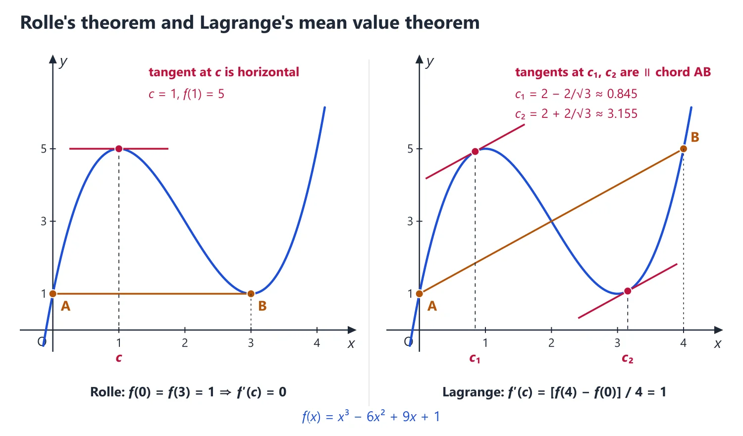
If f is continuous on [a, b], differentiable on (a, b) and f(a) = f(b), then f′(c) = 0 for some c ∈ (a, b).
Idea: a smooth curve that starts and ends at the same height must have a horizontal tangent somewhere in between, at a highest or lowest point (see the figure above). Proved in Standard Proofs, Theorem 5.
Each hypothesis is needed: |x| on [−1, 1] is not differentiable at 0 and has no such c.
Continuity at the end points is also needed: f(x) = x on [0, 1) with f(1) = 0 has f(0) = f(1), yet f′ = 1 throughout (0, 1). Equal end values are needed: f(x) = x on [0, 1] satisfies the other two conditions and f′ = 1.
Root between roots (method): to show that g(x) = 0 has a root between two roots of F(x) = 0, find φ with the same zeros as F (often e−xF, F/cos x or similar) whose derivative is a non-vanishing multiple of g, and apply Rolle's theorem to φ.
3. Understanding the Mean Value Theorems
Why we need it: we often know facts about f′ (it is positive, or at most 1/2) and want facts about f itself (it increases, or changes by at most half the change in x).
The mean value theorem (MVT) is the bridge from the derivative at one point to the change of f over an interval.
In words: (f(b) − f(a))/(b − a) is the average rate of change of f over [a, b], the slope of the chord.
Lagrange's MVT says that this average rate equals the instantaneous rate f′(c) at some interior point c, under the same continuity and differentiability hypotheses as Rolle (but without f(a) = f(b)).
In the form f(a + h) = f(a) + hf′(a + θh), the unknown point is written as a + θh with 0 < θ < 1; θ depends on f, a and h.
Cauchy's MVT compares two functions: the ratio of their changes equals the ratio of their derivatives at one common point c.
First example, slowly: show that |sin b − sin a| ≤ |b − a| for all real a, b.
Step 1: if a = b both sides are 0. Otherwise let a < b (the inequality is symmetric).
Step 2: sin x is continuous on [a, b] and differentiable on (a, b), so Lagrange's MVT applies.
Step 3: sin b − sin a = (b − a) cos c for some c ∈ (a, b).
Step 4: |cos c| ≤ 1, so |sin b − sin a| ≤ |b − a|. We never needed to know c: only a bound on f′ over the whole interval.
Non-example: f(x) = |x| on [−1, 2] has chord slope (2 − 1)/3 = 1/3, but f′(x) is −1 or 1 wherever it exists, never 1/3.
The failing hypothesis is differentiability at the interior point 0.
Building up: tilt the picture. Subtract the chord from f: φ(x) = f(x) − f(a) − ((f(b) − f(a))/(b − a))(x − a).
Then φ(a) = φ(b) = 0, Rolle gives φ′(c) = 0, and φ′(c) = 0 is exactly f′(c) = chord slope (Standard Proofs, Theorem 6).
Cauchy's version uses φ = f − Kg with K the ratio of the changes, so that φ(a) = φ(b) (Theorem 7). From Lagrange: f′ ≥ 0 on an interval gives f increasing, and |f′| ≤ M gives |f(x) − f(y)| ≤ M|x − y|.
Where it is used: two-sided inequalities such as bounds for log, tan−1 or sin−1, finding θ and lim θ, monotonicity, and the proof of L'Hôpital's rule.
4. Mean Value Theorems
Lagrange's MVT: if f is continuous on [a, b] and differentiable on (a, b), then f(b) − f(a) = (b − a)f′(c) for some c ∈ (a, b). Equivalent form: f(a + h) = f(a) + hf′(a + θh), 0 < θ < 1.
Idea: at some interior point the tangent is parallel to the chord AB joining the end points (see the figure above); in terms of motion, the average velocity over a time interval is attained as an instantaneous velocity at some moment. The proof (Standard Proofs, Theorem 6) applies Rolle's theorem to f minus its chord, φ(x) = f(x) − f(a) − ((f(b) − f(a))/(b − a))(x − a).
Cauchy's MVT: if f, g are continuous on [a, b], differentiable on (a, b) and g′(x) ≠ 0 on (a, b), then (f(b) − f(a))/(g(b) − g(a)) = f′(c)/g′(c) for some c ∈ (a, b).
Idea: for the curve x = g(t), y = f(t), the left side is the slope of the chord and f′(c)/g′(c) the slope of a tangent, so this is Lagrange's theorem for a curve in parametric form (Standard Proofs, Theorem 7). The condition g′ ≠ 0 makes g(b) ≠ g(a) (by Rolle) and f′(c)/g′(c) defined.
Applying Lagrange's MVT separately to f and to g gives two different points c1, c2, so Cauchy's theorem cannot be obtained by dividing the two results.
Consequences: f′ = 0 on an interval ⇒ f is constant; f′ > 0 ⇒ f is strictly increasing; the MVT proves inequalities such as x/(1 + x) < log(1 + x) < x for x > 0.
Why it works: for any x < y in the interval, f(y) − f(x) = (y − x)f′(c) = 0. The interval matters: sgn x on ℝ − {0} has derivative 0 everywhere on its domain but is not constant.
Inequalities by the MVT (method): apply Lagrange's MVT to f on [a, b] to get f(b) − f(a) = (b − a)f′(c); if f′ is monotonic on [a, b], f′(c) lies strictly between f′(a) and f′(b), which gives both bounds at once.
5. Understanding Taylor's Theorem
Why we need it: polynomials are easy to compute, differentiate and compare. We want to replace a complicated function near a point by a polynomial and know how large the error is.
The MVT is the first step (f is approximately constant, with error hf′); Taylor's theorem continues to any order.
In words: the Taylor polynomial of degree n − 1 about a is the unique polynomial whose value and first n − 1 derivatives at a agree with those of f.
The coefficient of hk is f(k)(a)/k!, because differentiating hk k times gives k!.
The remainder Rn is whatever is left over. Lagrange's form says it equals the next term, hnf(n)/n!, but with the n-th derivative taken at an unknown point a + θh.
So a bound |f(n)| ≤ M on the interval gives |Rn| ≤ M|h|n/n!.
First example, slowly: approximate √(1.2) by a degree-2 Taylor polynomial of f(x) = √x about a = 1 and bound the error.
Step 1 (derivatives): f = x1/2, f′ = (1/2)x−1/2, f″ = −(1/4)x−3/2, f‴ = (3/8)x−5/2. At x = 1: f = 1, f′ = 1/2, f″ = −1/4.
Step 2 (polynomial): with h = 0.2, √(1.2) ≈ 1 + (1/2)(0.2) − (1/8)(0.04) = 1 + 0.1 − 0.005 = 1.095.
Step 3 (remainder, n = 3): R3 = (h3/3!)f‴(1 + θh) = (0.008/6)(3/8)(1 + 0.2θ)−5/2.
Step 4 (bound): (1 + 0.2θ)−5/2 is at most 1, so 0 < R3 ≤ 0.0005. Hence 1.095 < √(1.2) ≤ 1.0955; the true value is 1.09545...
Notice that the sign of the remainder told us the approximation is too small.
Non-example: f(x) = |x|3 has f(0) = f′(0) = f″(0) = 0, but f‴(0) does not exist (f″(x) = 6|x|).
Taylor's theorem with n = 3 still applies about 0, since f″ is continuous and f‴ exists on (0, h). But f‴(0) does not exist, so the Taylor polynomial of degree 3 about 0 is not defined, and f has no Maclaurin series.
Even when all derivatives exist the series may fail: for e−1/x2 it is 0. The condition that must be checked is Rn → 0.
Building up: build an auxiliary function that equals f(b) at both ends, using the Taylor polynomial with a moving centre x plus a correcting term A(b − x)p.
Its derivative telescopes to a single term, Rolle's theorem makes it vanish at some c, and solving for A gives the remainder; p = n gives Lagrange's form, p = 1 Cauchy's (derived below and in Standard Proofs, Theorem 8).
Where it is used: series expansions of composite functions, approximate values to a stated accuracy, limits by expansion, the higher derivative test for extrema, and error terms in Numerical Analysis.
6. Taylor's Theorem with Remainders
If f(n−1) is continuous on [a, a + h] and f(n) exists on (a, a + h), then f(a + h) = f(a) + hf′(a) + (h2/2!)f″(a) + ... + (hn−1/(n − 1)!)f(n−1)(a) + Rn, where for some θ ∈ (0, 1):
Idea: the Taylor polynomial is the polynomial of degree n − 1 that matches f and its first n − 1 derivatives at a; the remainder Rn is the error, and the Lagrange form says that the error looks like the next term with f(n) evaluated at an unknown intermediate point. The Lagrange form is proved in Standard Proofs, Theorem 8.
Lagrange form: Rn = (hn/n!) f(n)(a + θh).
Cauchy form: Rn = (hn(1 − θ)n−1/(n − 1)!) f(n)(a + θh).
Schlömilch-Roche form: Rn = (hn(1 − θ)n−p/(p·(n − 1)!)) f(n)(a + θh) with p > 0; p = n gives the Lagrange form and p = 1 the Cauchy form.
Derivation of the general remainder: let b = a + h and φ(x) = f(x) + (b − x)f′(x) + ... + ((b − x)n−1/(n − 1)!)f(n−1)(x) + A(b − x)p, with A chosen so that φ(a) = f(b); also φ(b) = f(b).
The sum telescopes as in Standard Proofs, Theorem 8, so φ′(x) = ((b − x)n−1/(n − 1)!)f(n)(x) − pA(b − x)p−1. Rolle's theorem gives φ′(c) = 0 at c = a + θh, where b − c = h(1 − θ) ≠ 0, so A = (h(1 − θ))n−pf(n)(a + θh)/(p·(n − 1)!).
The equation φ(a) = f(a + h) is Taylor's formula with Rn = Ahp = (hn(1 − θ)n−p/(p·(n − 1)!))f(n)(a + θh). The value of θ depends on p, n and h, so the θ of the Lagrange form and of the Cauchy form are in general different numbers.
Maclaurin's theorem: put a = 0, h = x. The infinite series converges to f(x) exactly when Rn → 0 as n → ∞.
Why Rn → 0 must be checked: f(x) = e−1/x2 (with f(0) = 0) has f(n)(0) = 0 for every n, so its Maclaurin series is identically 0 while f(x) > 0 for x ≠ 0. For ex, |Rn| = |x|neθx/n! ≤ |x|ne|x|/n! → 0 for every x, so the series is valid on all of ℝ.
Standard expansions: ex = 1 + x + x2/2! + ...; sin x = x − x3/3! + x5/5! − ...; cos x = 1 − x2/2! + x4/4! − ...; log(1 + x) = x − x2/2 + x3/3 − ... (−1 < x ≤ 1); (1 + x)m = 1 + mx + m(m − 1)x2/2! + ... (|x| < 1).
Composite series: for functions such as ex cos x or log(1 + sin x), substitute the series of the inner function into that of the outer one and keep powers up to the required order; the coefficient of xn is f(n)(0)/n!.
Expansion about x = 1: log x = (x − 1) − (x − 1)2/2 + (x − 1)3/3 − ... for 0 < x ≤ 2. For an alternating series with terms decreasing to 0, the error after any term is less than the first omitted term.
7. Understanding Indeterminate Forms and L'Hôpital's Rule
Why we need it: the rule 'limit of a quotient = quotient of the limits' breaks down when both limits are 0 or both are infinite.
The answer then depends on how fast numerator and denominator move, and we need a systematic way to compare those speeds.
In words: a form is indeterminate when knowing the limits of the pieces is not enough to know the limit of the whole.
For 0/0: x/x → 1, x2/x → 0 and x/x3 → ∞ as x → 0, although every numerator and denominator tends to 0.
L'Hôpital's rule replaces the ratio of the values by the ratio of the rates: if f, g → 0 (or g → ∞) and f′/g′ has a limit l, then f/g → l.
The other forms 0·∞, ∞ − ∞, 00, 1∞, ∞0 are first rewritten as 0/0 or ∞/∞, by moving a factor into the denominator, combining fractions, or taking logarithms.
First example, slowly: find limx→0+ xx (form 00).
Step 1: let y = xx, so log y = x log x, a 0·∞ form (x → 0, log x → −∞).
Step 2: rewrite as a quotient: x log x = (log x)/(1/x), now of the form ∞/∞.
Step 3: L'Hôpital: (1/x)/(−1/x2) = −x → 0. So log y → 0.
Step 4: y = elog y and et is continuous, so y → e0 = 1. Always undo the logarithm at the end.
Non-example: limx→0 (1 + x)/(2 + x) = 1/2 is not indeterminate.
Applying the rule anyway gives 1/1 = 1, which is wrong: the hypothesis 'f, g → 0 or g → ∞' fails, so the rule says nothing.
Building up: for 0/0 at a, define f(a) = g(a) = 0 and apply Cauchy's MVT on [a, x]: f(x)/g(x) = f′(c)/g′(c) with c between a and x.
As x → a, c is squeezed to a, so f(x)/g(x) has the same limit as f′/g′ (derived in full below).
Taylor expansions give the same answers and show why: if f = αxk + ... and g = βxk + ... with β ≠ 0, then f/g → α/β, the ratio of the first non-zero terms.
Where it is used: 10-mark limit questions, finding constants that make a limit finite, the 'value that makes f continuous', asymptote intercepts and limits in improper integrals.
8. Indeterminate Forms
L'Hôpital's rule: if f(x), g(x) → 0 (or both → ∞) as x → a, f and g are differentiable near a with g′(x) ≠ 0, and lim f′(x)/g′(x) = l exists (finite or infinite), then lim f(x)/g(x) = l.
Derivation (0/0 case, x → a+): set f(a) = g(a) = 0, so f and g are continuous on [a, x]. Cauchy's MVT gives f(x)/g(x) = (f(x) − f(a))/(g(x) − g(a)) = f′(c)/g′(c) for some c ∈ (a, x); as x → a+, c → a+, so f(x)/g(x) → l. The left-hand limit is handled the same way.
Idea: near a, f and g behave like their tangent lines f′(a)(x − a) and g′(a)(x − a), so their ratio behaves like the ratio of the slopes.
0·∞: write f·g as f/(1/g). ∞ − ∞: combine into one fraction. 00, 1∞, ∞0: put y = fg, find L = lim g log f; the limit is eL.
Why the logarithm works: fg = eg log f and ex is continuous, so lim fg = elim g log f. For 1∞ a shortcut is lim fg = elim g(f − 1), because (log f)/(f − 1) → 1 as f → 1; for example limx→0 (1 + sin x)1/x = elim (sin x)/x = e.
A series expansion is often faster than repeated L'Hôpital; check that the form is still indeterminate before each application.
Finding constants: to make limx→0 (expression)/xn finite, expand the numerator in powers of x; the coefficients of x0, ..., xn−1 must vanish, and the coefficient of xn is then the limit.
A standard 0·∞ limit: limx→a (a − x) tan(πx/2a) = 2a/π, obtained by writing the product as (a − x)/cot(πx/2a) and applying L'Hôpital's rule.
9. Choosing the Method
If an inequality involving f(b) − f(a) and b − a is asked (log, tan−1, sin−1, ex) → Lagrange's MVT on [a, b], with the monotonicity of f′ giving both bounds.
If a ratio of two differences (f(b) − f(a))/(g(b) − g(a)) appears → Cauchy's MVT, with g the function in the denominator (often x2, 1/x, log x or ex).
If a root between two roots is asked → Rolle's theorem on a suitable product or antiderivative; if exactly one root is asked → existence by the intermediate value theorem and uniqueness by Rolle (two roots would force f′ = 0 between them).
If θ in f(a + h) = f(a) + hf′(a + θh) or its limit as h → 0 is asked → solve for θ directly; when f″ is continuous at a with f″(a) ≠ 0, comparing with the second-order Taylor formula gives limh→0 θ = 1/2.
If a 0/0 limit involves sin, tan, ex, log(1 + x) or (1 + x)m → Maclaurin expansions to the first non-vanishing order are usually faster and safer than repeated L'Hôpital; if the form is 1∞, 00 or ∞0 → take logarithms first.
If a series expansion of a composite function is asked → substitute known series; if a general coefficient is asked → obtain a recurrence for f(n)(0) by differentiating a relation such as (1 + x)y′ = my (Leibniz's theorem).
10. Common Mistakes
Applying L'Hôpital's rule to a form that is not 0/0 or ∞/∞: limx→0 (cos x)/(x + 1) = 1, but differentiating top and bottom gives the wrong value 0.
Differentiating f/g by the quotient rule instead of differentiating f and g separately.
Concluding that lim f/g does not exist because lim f′/g′ does not: (x + sin x)/x → 1 as x → ∞, although (1 + cos x)/1 oscillates.
Using Rolle's theorem or the MVT without checking the hypotheses: x2/3 on [−1, 1] has equal end values but is not differentiable at 0, and f′(x) = (2/3)x−1/3 never vanishes.
Treating θ as independent of h, or using one c for f and another for g in Cauchy's MVT.
Using a Maclaurin series outside its range: log(1 + x) = x − x2/2 + ... needs −1 < x ≤ 1, and the binomial series needs |x| < 1.
11. Connections
Link: the Lagrange remainder gives the error terms of interpolation formulae and of the trapezoidal and Simpson's rules, and the second-order Taylor expansion gives the quadratic convergence of Newton-Raphson (Numerical Analysis).
Link: in Complex Analysis a function differentiable in a disc always equals its Taylor series there, in sharp contrast with e−1/x2 on ℝ.
Link: the MVT is the bridge from derivatives to monotonicity and bounds throughout Real Analysis (uniform continuity from a bounded derivative, term-by-term differentiation of series).
12. Worked Examples
Example 1: Evaluate limx→0 (x − sin x)/x3.
x − sin x = x3/6 − x5/120 + ..., so the limit is 1/6; three applications of L'Hôpital's rule give the same value.
Example 2: Evaluate limx→0 (1/x2 − 1/sin2x).
The expression equals (sin2x − x2)/(x2 sin2x). Since sin2x = x2 − x4/3 + ..., the numerator behaves like −x4/3 and the denominator like x4, so the limit is −1/3.
Example 3: Evaluate limx→0 (cos x)1/x2.
log y = (log cos x)/x2, and by L'Hôpital lim (−tan x)/(2x) = −1/2, so the limit is e−1/2.
Example 4: For f(x) = x3, find θ in f(h) = f(0) + hf′(θh). Here h3 = h·3θ2h2, so θ = 1/√3, which lies in (0, 1).
Example 5: Prove x/(1 + x) < log(1 + x) < x for x > 0. Lagrange's MVT for log t on [1, 1 + x] gives log(1 + x) = x/c with 1 < c < 1 + x, and 1/(1 + x) < 1/c < 1 gives the result.
Example 6: Using Maclaurin's theorem with Lagrange's remainder, show that log(1 + x) = x − x2/2 + x3/3 − ... for 0 ≤ x ≤ 1, and deduce log 2 = 1 − 1/2 + 1/3 − ...
For f(x) = log(1 + x), f(n)(x) = (−1)n−1(n − 1)!/(1 + x)n, so f(n)(0) = (−1)n−1(n − 1)!.
Lagrange's remainder: Rn = (xn/n!) f(n)(θx) = (−1)n−1 xn/(n(1 + θx)n), 0 < θ < 1.
For 0 ≤ x ≤ 1, 0 ≤ x/(1 + θx) ≤ 1, so |Rn| ≤ 1/n → 0, and the Maclaurin series converges to log(1 + x). Putting x = 1 gives log 2 = 1 − 1/2 + 1/3 − ...
For −1 < x < 0 this bound fails; there one uses Cauchy's form of the remainder.
13. Solved UPSC Questions
Example 7 (UPSC 2014, 10 marks): Prove that between two real roots of ex cos x + 1 = 0, a real root of ex sin x + 1 = 0 lies.
Let φ(x) = e−x + cos x. Since ex > 0, ex cos x + 1 = exφ(x) = 0 ⇔ φ(x) = 0.
Let α < β be real roots of ex cos x + 1 = 0. Then φ(α) = φ(β) = 0, and φ is continuous on [α, β] and differentiable on (α, β); by Rolle's theorem φ′(c) = 0 for some c ∈ (α, β).
φ′(x) = −e−x − sin x = −e−x(1 + ex sin x), so φ′(c) = 0 gives ec sin c + 1 = 0.
Answer: c ∈ (α, β) is a root of ex sin x + 1 = 0, as required.
Example 8 (UPSC 2021, 10 marks): Show that between any two roots of ex cos x = 1, there exists at least one root of ex sin x − 1 = 0.
Let ψ(x) = e−x − cos x. Then ex cos x = 1 ⇔ cos x = e−x ⇔ ψ(x) = 0.
If α < β are roots of ex cos x = 1, then ψ(α) = ψ(β) = 0 and ψ is differentiable on ℝ, so Rolle's theorem gives c ∈ (α, β) with ψ′(c) = 0.
ψ′(x) = −e−x + sin x = e−x(ex sin x − 1), so ψ′(c) = 0 gives ec sin c − 1 = 0.
Answer: Between any two roots of ex cos x = 1 there is a root c of ex sin x − 1 = 0.
Example 9 (UPSC 2018, 10 marks): Determine if limz→1 (1 − z) tan(πz/2) exists or not. If the limit exists, then find its value.
As z → 1, 1 − z → 0 and tan(πz/2) → ±∞: the form is 0·∞. Write (1 − z) tan(πz/2) = [(1 − z)/cos(πz/2)] · sin(πz/2).
(1 − z)/cos(πz/2) is a 0/0 form; by L'Hôpital's rule it tends to lim (−1)/(−(π/2) sin(πz/2)) = 2/π, and sin(πz/2) → 1.
(Check: with z = 1 − t, tan(π/2 − πt/2) = cot(πt/2), and t cot(πt/2) = (2/π)·(πt/2)/tan(πt/2) → 2/π from both sides.)
Answer: The limit exists and equals 2/π.
Example 10 (UPSC 2022, 10 marks): Evaluate limx→∞ (ex + x)1/x.
Let y = (ex + x)1/x (form ∞0), so log y = log(ex + x)/x, of the form ∞/∞.
By L'Hôpital's rule, lim log y = lim (ex + 1)/(ex + x) = lim (1 + e−x)/(1 + xe−x) = 1, since e−x → 0 and xe−x → 0.
(Directly: log(ex + x) = x + log(1 + xe−x), so log y = 1 + log(1 + xe−x)/x → 1.)
Answer: limx→∞ (ex + x)1/x = e.
Example 11 (UPSC 2023, 10 marks): Find the values of p and q for which limx→0 [x(1 + p cos x) − q sin x]/x3 exists and equals 1.
With cos x = 1 − x2/2 + O(x4) and sin x = x − x3/6 + O(x5): x(1 + p cos x) − q sin x = (1 + p − q)x + (−p/2 + q/6)x3 + O(x5).
After dividing by x3, the limit is finite only if 1 + p − q = 0, and then it equals −p/2 + q/6.
So q = 1 + p and −p/2 + (1 + p)/6 = 1, i.e. −3p + 1 + p = 6, giving p = −5/2 and q = −3/2.
Check: x − (5/2)x cos x + (3/2) sin x = x − (5/2)x + (5/4)x3 + (3/2)x − (1/4)x3 + O(x5) = x3 + O(x5).
Answer: p = −5/2, q = −3/2.
Example 12 (UPSC 2024, 10 marks): Expand ln(x) in powers of (x − 1) by Taylor's theorem and hence find the value of ln(1·1) correct up to four decimal places.
For f(x) = ln x, f(n)(x) = (−1)n−1(n − 1)!/xn, so f(1) = 0 and f(n)(1)/n! = (−1)n−1/n.
Taylor's theorem about 1 with h = x − 1: ln x = h − h2/2 + h3/3 − ... + (−1)nhn−1/(n − 1) + Rn, where the Lagrange remainder is Rn = (−1)n−1hn/(n(1 + θh)n); for 0 ≤ h ≤ 1, |Rn| ≤ hn/n → 0.
For x = 1.1, h = 0.1: ln 1.1 = 0.1 − 0.005 + 0.000333 − 0.000025 + 0.000002 − ... ; with four terms, |R5| ≤ (0.1)5/5 = 0.000002.
Sum of four terms: 0.1 − 0.005 + 0.0003333 − 0.000025 = 0.0953083, and the true value lies between 0.0953083 and 0.0953103.
Answer: ln x = (x − 1) − (x − 1)2/2 + (x − 1)3/3 − ... (0 < x ≤ 2); ln 1.1 = 0.0953 to four decimal places.
Example 13 (UPSC 2025, 15 marks): Using Mean Value Theorem, prove that
π/6 + √3/15 < sin−1(3/5) < π/6 + 1/8.
Apply Lagrange's MVT to f(x) = sin−1x on [1/2, 3/5]; f is continuous there and differentiable on the open interval with f′(x) = 1/√(1 − x2).
So sin−1(3/5) − sin−1(1/2) = (3/5 − 1/2)/√(1 − c2) = 1/(10√(1 − c2)) for some c ∈ (1/2, 3/5), and sin−1(1/2) = π/6.
1/√(1 − x2) increases on (0, 1), so 1/√(1 − 1/4) < 1/√(1 − c2) < 1/√(1 − 9/25), i.e. 2/√3 < 1/√(1 − c2) < 5/4.
Dividing by 10: √3/15 = 2/(10√3) < sin−1(3/5) − π/6 < 5/40 = 1/8.
Answer: π/6 + √3/15 < sin−1(3/5) < π/6 + 1/8.
Example 14 (UPSC 2026, 10 marks): Using Maclaurin's theorem, obtain the first four terms of the expansion of ex cos x in ascending powers of x. Hence or otherwise find the limit of (ex − ex cos x)/(x − sin x) as x tends to zero.
u = x cos x = x − x3/2 + O(x5), so u2 = x2 + O(x4) and u3 = x3 + O(x5). In eu = 1 + u + u2/2 + u3/6 + O(u4):
ex cos x = 1 + (x − x3/2) + x2/2 + x3/6 + O(x4) = 1 + x + x2/2 − x3/3 + O(x4). By Maclaurin's theorem these are f(0), f′(0)x, f″(0)x2/2! and f‴(0)x3/3! for f(x) = ex cos x.
ex − ex cos x = (1 + x + x2/2 + x3/6) − (1 + x + x2/2 − x3/3) + O(x4) = x3/2 + O(x4), and x − sin x = x3/6 + O(x5).
Hence the ratio is (1/2 + O(x))/(1/6 + O(x2)) → 3.
Answer: ex cos x = 1 + x + x2/2 − x3/3 + ...; the limit is 3.
14. Practice Exercises
Exercise 1 (basic): Verify Rolle's theorem for f(x) = x2 − 5x + 6 on [2, 3].
Answer: f(2) = f(3) = 0, f is a polynomial, and f′(c) = 2c − 5 = 0 gives c = 5/2 ∈ (2, 3).
Exercise 2 (basic): Find the point c of Lagrange's MVT for f(x) = x3 on [0, 2].
Answer: 8 − 0 = 2·3c2, so c2 = 4/3 and c = 2/√3 ≈ 1.155 ∈ (0, 2).
Exercise 3 (basic): Evaluate limx→0 (ex − 1 − x)/x2.
Answer: 1/2 (numerator = x2/2 + x3/6 + ...).
Exercise 4 (standard): Prove that (b − a)/b < log(b/a) < (b − a)/a for 0 < a < b.
Answer: Lagrange's MVT for log x on [a, b]: log b − log a = (b − a)/c with a < c < b, and 1/b < 1/c < 1/a.
Exercise 5 (standard): Evaluate limx→0 (tan x − x)/(x − sin x).
Answer: 2, since tan x − x = x3/3 + ... and x − sin x = x3/6 + ...
Exercise 6 (standard): Evaluate limx→0 (1/x − 1/(ex − 1)).
Answer: combine: (ex − 1 − x)/(x(ex − 1)) = (x2/2 + ...)/(x2 + ...) → 1/2.
Exercise 7 (standard): Expand ex sin x in powers of x up to the term in x5.
Answer: x + x2 + x3/3 − x5/30 + ... (the x4 coefficient is 0).
Exercise 8 (standard): Show that x3 − 3x + c = 0 cannot have two distinct roots in (0, 1), whatever the real number c.
Answer: two roots in (0, 1) would give, by Rolle, a zero of 3x2 − 3 in (0, 1); but 3x2 − 3 < 0 there.
Exercise 9 (UPSC level): For f(x) = 1/x, a = 1 and h > 0, find θ in f(a + h) = f(a) + hf′(a + θh) and show that θ → 1/2 as h → 0.
Answer: 1/(1 + h) − 1 = −h/(1 + θh)2 gives (1 + θh)2 = 1 + h, θ = (√(1 + h) − 1)/h = 1/(√(1 + h) + 1) → 1/2.
Exercise 10 (UPSC level): Find a, b, c such that limx→0 (aex − b cos x + ce−x)/(x sin x) = 2.
Answer: the constant and x coefficients must vanish: a − b + c = 0, a − c = 0; the x2 coefficient (a + b + c)/2 must equal 2. So a = 1, b = 2, c = 1.
Exercise 11 (UPSC level): Using Maclaurin's theorem with Lagrange's remainder, show that |sin x − (x − x3/6)| ≤ |x|5/120, and hence find sin(0.2) to five decimal places. Also evaluate limx→0 ((1 + x)1/x/e)1/x.
Answer: the x4 term is 0, so R5 = (x5/120) cos θx; sin(0.2) ≈ 0.2 − 0.0013333 = 0.198667, and the remainder is positive and at most 0.0000027, so sin(0.2) = 0.19867. The limit is e−1/2, since (1/x)(log(1 + x)/x − 1) → −1/2.
| Form | Conversion | Example |
|---|---|---|
| 0/0 | L'Hôpital or series directly | limx→0 (x − sin x)/x3 = 1/6 |
| ∞/∞ | L'Hôpital directly | limx→∞ xn/ex = 0 |
| 0·∞ | f·g = f/(1/g) | limx→0+ x log x = 0 |
| ∞ − ∞ | Single fraction | limx→0 (1/x2 − 1/sin2x) = −1/3 |
| 1∞ | elim g log f | limx→0 (cos x)1/x2 = e−1/2 |
| 00 | elim g log f | limx→0+ xx = 1 |
| ∞0 | elim g log f | limx→∞ x1/x = 1 |
Mains points
- Common questions: verify Rolle's or Lagrange's theorem for a given function on an interval and find c; prove an inequality using the MVT.
- Taylor's theorem questions ask for an expansion with a stated remainder form, or for lim θ as h → 0 in f(a + h) = f(a) + hf′(a) + (h2/2)f″(a + θh); expand both sides further and compare coefficients.
- Before applying L'Hôpital's rule, write the form (0/0 or ∞/∞) in the answer; examiners deduct marks when the rule is used on a determinate form.
- For exponential forms, take logarithms first and state the final answer as eL.
- Check every hypothesis (continuity on the closed interval, differentiability on the open interval) before quoting a mean value theorem; questions often hide a point where one fails.
Did you know?
- L'Hôpital's rule was discovered by Johann Bernoulli, who sold his results to the Marquis de l'Hôpital; the rule appeared in l'Hôpital's 1696 textbook, the first calculus textbook.
Maxima and Minima, Asymptotes and Curve Tracing
Local extrema of f occur where f′ = 0 or f′ does not exist and are classified by the first or higher derivative test. Asymptotes of algebraic curves are found from the highest-degree terms (slopes) and the next terms (intercepts). Curve tracing combines symmetry, the origin, intercepts, asymptotes, regions of existence and monotonicity.
1. Understanding Local Extrema and the Derivative Tests
Why we need it: optimisation questions (largest volume, least cost, shortest distance) ask for the best value of a quantity. Checking every x is impossible, so we need a short list of candidates and a way to judge each one.
In words: f has a local maximum at c if f(c) ≥ f(x) for all x in some interval around c; 'local' means only nearby points are compared.
An absolute maximum on a set compares c with every point of the set. A local maximum need not be absolute, and an absolute maximum on [a, b] may sit at an end point, where f′ need not vanish.
A critical point is an interior point where f′ = 0 or f′ does not exist. Every interior local extremum is a critical point, so the candidates are: critical points and end points.
The first derivative test reads the sign of f′ on the two sides: rising then falling (+ to −) means a peak; falling then rising (− to +) means a valley.
The second derivative test reads the bending at c: f′(c) = 0 and f″(c) < 0 means the graph is cap-shaped there (maximum); f″(c) > 0 means cup-shaped (minimum).
First example, slowly: find the absolute extrema of f(x) = x3 − 3x on [0, 2].
Step 1 (critical points): f′(x) = 3x2 − 3 = 3(x − 1)(x + 1). In the open interval (0, 2) only x = 1 qualifies; x = −1 lies outside.
Step 2 (classify): f″(x) = 6x, so f″(1) = 6 > 0, a local minimum. Check by signs: f′ < 0 on (0, 1) and f′ > 0 on (1, 2), − to +.
Step 3 (values): f(0) = 0, f(1) = −2, f(2) = 8 − 6 = 2.
Step 4 (compare): the absolute minimum is −2 at x = 1 and the absolute maximum is 2 at the end point x = 2, where f′(2) = 9 ≠ 0. The end point had to be checked separately.
Non-example: f(x) = x3 at 0 has f′(0) = 0 but no extremum: f′ = 3x2 is positive on both sides, so f keeps rising through 0.
The condition that fails is the sign change of f′. Here f″(0) = 0 and f‴(0) = 6 ≠ 0, the first non-zero derivative has odd order, and 0 is a point of inflexion.
Building up: the first derivative test follows from the MVT: f′ > 0 on (c − δ, c) makes f increasing up to c, and f′ < 0 on (c, c + δ) makes it decreasing after c, so f(c) is the largest nearby value.
The higher derivative test follows from Taylor's theorem: near c, f(c + h) − f(c) behaves like (hn/n!)f(n)(c), whose sign is fixed for even n and flips with h for odd n (derived below).
Where it is used: 10 to 20-mark optimisation questions on cones, cylinders, boxes and triangles, extreme values on a closed interval, stability of equilibrium in Statics, and as the model for the Hessian test in several variables.
2. Maxima and Minima (One Variable)
f has a local maximum at c if f(c) ≥ f(x) in some neighbourhood of c. Necessary condition: if f is differentiable at an interior extremum c, then f′(c) = 0.
Why f′(c) = 0: if f′(c) > 0, the quotient (f(c + h) − f(c))/h is positive for small h, so f(c + h) > f(c) for small h > 0, which contradicts a maximum; f′(c) < 0 fails in the same way. The condition is not sufficient (x3 at 0) and an extremum may occur where f′ does not exist (|x| at 0).
First derivative test: if f′ changes sign from + to − at c, f has a maximum; from − to +, a minimum; if f′ does not change sign, neither.
Higher derivative test: if f′(c) = f″(c) = ... = f(n−1)(c) = 0 and f(n)(c) ≠ 0, then for n even there is a maximum if f(n)(c) < 0 and a minimum if f(n)(c) > 0; for n odd there is no extremum (c is a point of inflexion).
Derivation: Taylor's theorem gives f(c + h) − f(c) = (hn/n!)f(n)(c + θh). If f(n) is continuous at c, f(n)(c + θh) has the sign of f(n)(c) for small h; for even n, hn > 0 on both sides (an extremum), while for odd n, hn changes sign with h (no extremum).
Idea: f″(c) > 0 means the graph bends upward like a cup, so a horizontal tangent there sits at a bottom; x4 needs the fourth derivative at 0 because f′ = f″ = f‴ = 0 there.
Absolute extrema on [a, b]: compare the values of f at the critical points (f′ = 0 or f′ undefined) and at the end points a, b.
Optimisation problems (method): (1) name the variables and write the quantity to optimise; (2) use the constraint to reduce it to one variable on its natural interval; (3) solve f′ = 0; (4) confirm with f″ or by comparing end values; (5) answer exactly what is asked (a ratio, an angle, a height).
Monotone case: if f′ does not vanish inside [a, b], f is monotonic there and its maximum and minimum occur at the end points.
Functions defined by integrals: for f(x) = ∫ax g(t) dt with g continuous, f′(x) = g(x); the critical points are the zeros of g, and the sign of g decides where f increases or decreases.
3. Understanding Asymptotes
Why we need it: a sketch of a curve is incomplete without knowing what its infinite branches do. Asymptotes are the lines that the far-away parts of the curve approach, and they fix the shape of the sketch at the edges.
In words: a line L is an asymptote if, as a point P moves along a branch of the curve to infinity, the perpendicular distance from P to L tends to 0.
Three kinds occur. Vertical: x = k, where y → ±∞ as x → k. Horizontal: y = k, where y → k as x → ±∞. Oblique: y = mx + c with m ≠ 0, where y − (mx + c) → 0 as x → ±∞.
For an oblique asymptote of y = f(x), the slope is m = lim f(x)/x and the intercept is c = lim (f(x) − mx), both taken as x → ∞ (or as x → −∞).
For an algebraic curve the same two limits are packaged as φn(m) = 0 and c = −φn−1(m)/φn′(m): the highest-degree terms decide the directions and the next terms the positions.
First example, slowly: find the asymptotes of y = (2x2 + 3x − 1)/(x − 1).
Step 1 (vertical): the denominator vanishes at x = 1, and the numerator there is 2 + 3 − 1 = 4 ≠ 0, so y → ±∞ as x → 1: x = 1 is a vertical asymptote.
Step 2 (slope): m = lim y/x = lim (2x2 + 3x − 1)/(x2 − x) = 2.
Step 3 (intercept): y − 2x = (2x2 + 3x − 1 − 2x2 + 2x)/(x − 1) = (5x − 1)/(x − 1) → 5, so c = 5.
Step 4 (check by division): 2x2 + 3x − 1 = (2x + 5)(x − 1) + 4, so y = 2x + 5 + 4/(x − 1), and the last term → 0. The asymptotes are x = 1 and y = 2x + 5.
Step 5 (side of approach): for large positive x, 4/(x − 1) > 0, so the curve lies just above the line; for large negative x it lies just below. Such details make the sketch correct.
Non-example: the parabola y = x2 goes to infinity but has no asymptote.
Here y/x = x → ∞, so no finite slope m exists. Similarly y = x + √|x| has slope limit m = 1, but y − x = √|x| → ∞, so the intercept condition fails and y = x + c is not an asymptote for any c.
Building up: substituting y = mx + c into an algebraic equation of degree n gives an equation in x whose leading coefficients are φn(m) and cφn′(m) + φn−1(m).
A line meets the curve 'twice at infinity', which is what an asymptote does, exactly when both coefficients vanish; this is the derivation given below.
Asymptotes parallel to the axes are the special directions in which m is infinite or 0, and they come from the coefficients of the highest powers of y and x. For polar curves, r → ∞ when 1/r = f(θ) → 0, which gives r sin(θ − θ1) = 1/f′(θ1).
Where it is used: 'find all the asymptotes' questions (10 marks), every curve-tracing question, and the asymptotes of hyperbolas and asymptotic cones in Analytic Geometry.
4. Asymptotes
A straight line is an asymptote of a curve if the distance from a point on the curve to the line tends to 0 as the point moves to infinity along the curve.
Idea: an asymptote is the line that a branch of the curve hugs far away. The curve may cross its asymptote, even infinitely often (y = (sin x)/x crosses y = 0 at every x = kπ, k ≠ 0); only the distance tending to 0 matters.
Oblique asymptotes y = mx + c of an algebraic curve of degree n: let φk(m) be the k-th degree part of the equation with x = 1, y = m. Substituting y = mx + c gives xnφn(m) + xn−1[cφn′(m) + φn−1(m)] + ... = 0.
Solve φn(m) = 0 for m and take c = −φn−1(m)/φn′(m); if φn′(m) = 0 also, c is found from (c2/2)φn″(m) + cφn−1′(m) + φn−2(m) = 0, giving two parallel asymptotes.
Why it works: the abscissae of the points where the line y = mx + c meets the curve are the roots of the equation above. The line is an asymptote when two of these points have moved off to infinity, which happens exactly when the coefficients of xn and xn−1 both vanish: φn(m) = 0 and cφn′(m) + φn−1(m) = 0.
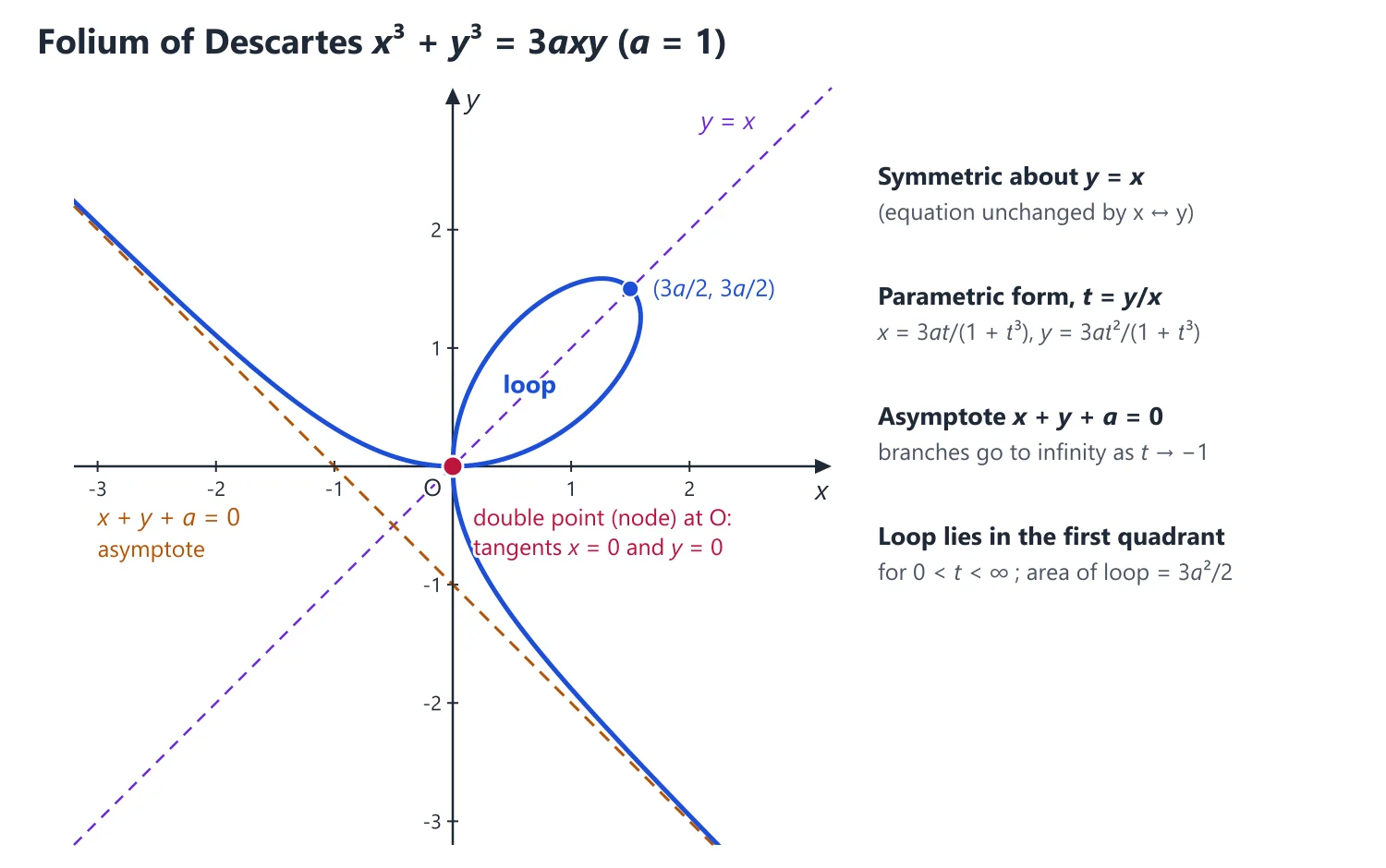
Example (figure above): for the folium x3 + y3 = 3axy, φ3(m) = 1 + m3 and φ2(m) = −3am, so m = −1 and c = −φ2(−1)/φ3′(−1) = −3a/3 = −a; the asymptote is x + y + a = 0.
Asymptotes parallel to the axes: equate to zero the coefficient of the highest power of x (this gives horizontal asymptotes y = k) and of y (vertical asymptotes x = k), when these coefficients are not constants.
An algebraic curve of degree n has at most n asymptotes.
Polar curves: if 1/r = f(θ), f(θ1) = 0 and f′(θ1) ≠ 0, the asymptote is r sin(θ − θ1) = 1/f′(θ1).
Derivation: as θ → θ1, r → ∞, so the branch goes off in the direction θ = θ1 and the asymptote is parallel to it. The distance of the pole from the asymptote is p = limθ→θ1 r sin(θ − θ1) = lim sin(θ − θ1)/f(θ) = 1/f′(θ1) by L'Hôpital, and the line parallel to θ = θ1 at this distance is r sin(θ − θ1) = 1/f′(θ1).
Rational functions: for y = P(x)/Q(x) in lowest terms, the zeros of Q give vertical asymptotes; if deg P = deg Q + 1, dividing P = (mx + c)Q + R gives the oblique asymptote y = mx + c; if deg P ≤ deg Q there is a horizontal asymptote.
5. Understanding Curve Tracing
Why we need it: an equation such as y2(a − x) = x3 hides its shape. Plotting many points is slow and misses the important features, so we read the shape from the equation in a fixed order of checks.
In words: curve tracing means finding the qualitative features that determine the picture: symmetry, behaviour at the origin, intercepts, asymptotes, where the curve exists, where it rises or falls, and special points.
A node is a point where two branches cross with different tangents; a cusp is a point where two branches meet with a common tangent and stop; an isolated (conjugate) point is a point of the curve with no other points of the curve near it.
Each item answers one question about the picture, and the items are independent, so a mistake in one does not spoil the others.
First example, slowly: trace y2 = x2(1 − x).
Step 1 (symmetry): only y2 occurs, so the curve is symmetric about the x-axis. Draw the upper half and reflect it.
Step 2 (origin): there is no constant term, so O is on the curve. The lowest-degree terms are y2 − x2, giving the tangents y = ±x: two real distinct tangents, so O is a node.
Step 3 (intercepts): y = 0 gives x = 0 or x = 1. At (1, 0) the curve crosses the axis vertically, because 1 − x changes sign there (a simple zero of the right side).
Step 4 (region): y2 ≥ 0 needs 1 − x ≥ 0, so the curve lies entirely in x ≤ 1.
Step 5 (asymptotes): the coefficient of y2 is the constant 1 and the cubic terms give φ3(m) = 1, which has no root; so there are no asymptotes.
Step 6 (shape): for 0 ≤ x ≤ 1, y = x√(1 − x) rises from 0 and falls back to 0, a loop between O and (1, 0). For x < 0, |y| = |x|√(1 − x) grows without bound, two branches going to infinity in the second and third quadrants.
Step 7 (special point): on the loop, dy/dx = (2 − 3x)/(2√(1 − x)) = 0 at x = 2/3, so the loop is widest at x = 2/3, where y = (2/3)√(1/3) = 2√3/9.
Non-example: for y2 = x2(x − 1) the lowest-degree terms y2 + x2 = 0 give no real tangents at O.
O still satisfies the equation, but near O we have x − 1 < 0, so no other point of the curve is near O: O is an isolated point, not a node, and the rest of the curve lies in x ≥ 1. Drawing branches through O would be wrong.
Building up: each step is a small theorem already met. Symmetry follows from the invariance of the equation, tangents at O from the lowest-degree terms dominating near O, asymptotes from the highest-degree terms dominating far away.
Rising and falling come from the sign of dy/dx (MVT), and concavity from the sign of d2y/dx2. For polar curves the same plan uses θ → −θ for symmetry, a table of r against θ, tan φ = r dθ/dr for directions, and the range of θ where r is real.
Where it is used: 15 to 20-mark tracing questions (strophoid, cissoid, folium, curves y2 = g(x)), and the first step of every area, arc length or volume question in the multiple-integrals topic, where the region must be identified correctly.
6. Curve Tracing
Step 1, symmetry: about the x-axis if only even powers of y occur; about the y-axis if only even powers of x occur; about the origin if the equation is unchanged by (x, y) → (−x, −y); about y = x if unchanged when x and y are interchanged.
Step 2, origin: the curve passes through the origin if there is no constant term; the tangents there are found by equating the lowest-degree terms to zero (two real distinct tangents: node; coincident: usually a cusp, but check the nearby branches, since a tacnode or an isolated point is also possible; imaginary: isolated point).
Why the lowest-degree terms: near the origin the higher-degree terms are negligible compared with the lowest-degree ones, so the curve looks like the lines given by those terms. For the folium x3 + y3 = 3axy the lowest terms give xy = 0, so the tangents at the node O are the two axes (see the figure above).
Steps 3 to 6: points of intersection with the axes and tangents there; asymptotes; regions where the curve does not exist (y2 < 0); the sign of dy/dx for increasing and decreasing parts, and points of inflexion.
Polar curves: symmetry about the initial line if the equation is unchanged by θ → −θ; tabulate r at θ = 0, π/4, π/2, ...; tan φ = r dθ/dr gives the angle between the radius vector and the tangent; note the range of θ for which r is real.
Parametric curves: find dx/dt and dy/dt, the points where each vanishes, and the behaviour as t runs over its range (for example the cycloid x = a(t − sin t), y = a(1 − cos t)).
Region of existence for y2 = g(x): make a sign table of g from the zeros of its numerator and denominator. The curve exists only where g(x) ≥ 0, crosses the x-axis with a vertical tangent at simple zeros of g, and has vertical asymptotes at zeros of the denominator.
Strophoid-type curves y2(a + x) = x2(b − x) (a, b > 0): a node at the origin with tangents ay2 = bx2, a loop for 0 ≤ x ≤ b, and two branches for −a < x < 0 approaching the asymptote x = −a.
7. Choosing the Method
If f″(c) is easy to compute and non-zero → second derivative test; if f″(c) = 0 or is messy → the sign change of f′ around c, or higher derivatives.
If the domain is a closed interval → compare the values at the critical points and at the end points; f″ alone does not give absolute extrema.
If a geometric optimisation is asked (largest cylinder in a sphere, shortest distance) → reduce to one variable, or use Lagrange multipliers when the constraint is symmetric (Functions of Several Variables).
If y = P(x)/Q(x) → vertical asymptotes from Q = 0 and the oblique one by division; if a general algebraic curve → the φn(m) method plus asymptotes parallel to the axes; if polar → r sin(θ − θ1) = 1/f′(θ1); if parametric → find t where x or y → ∞, then m = lim y/x and c = lim (y − mx).
If a curve is to be traced → follow the fixed order: symmetry, origin, intercepts, asymptotes, region of existence, monotonicity, special points, and record each item in the answer before drawing.
8. Common Mistakes
Missing critical points where f′ does not exist (|x − 1| at x = 1), or forgetting the end points of a closed interval.
Treating f″(c) = 0 as proof of a point of inflexion: x4 has f″(0) = 0 and a minimum at 0. An inflexion requires a change of concavity (a sign change of f″).
Forgetting the asymptotes parallel to the axes after using the φn(m) method, or listing more than n asymptotes for a curve of degree n.
Assuming the curve never meets its asymptote; the finite intersection points should be found, as they help the sketch.
Tracing a curve without stating where it does not exist (y2 < 0), or drawing branches in that region.
Stating 'maximum' or 'minimum' without a test, or answering with the point when the question asks for the value (or the reverse).
9. Connections
Link: in Statics an equilibrium position is stable when the potential energy has a minimum there, so the tests of this topic decide the stability of equilibrium.
Link: the f′ = 0 and f″ tests generalise to the gradient and Hessian tests for several variables, and the asymptotes of a hyperbola or the asymptotic cone of a hyperboloid come from the same highest-degree-terms idea (Analytic Geometry).
Link: Linear Programming optimises a linear function, whose derivative never vanishes, so the optimum lies on the boundary, at a vertex of the feasible region, just as in the monotone case above.
10. Worked Examples
Example 1: Find the asymptotes of the folium x3 + y3 = 3axy.
There are no asymptotes parallel to the axes, since the coefficients of x3 and y3 are constants. φ3(m) = 1 + m3 and φ2(m) = −3am; the real root of φ3(m) = 0 is m = −1, and c = −φ2(m)/φ3′(m) = 3am/(3m2) = a/m = −a. The asymptote is x + y + a = 0.
Tracing: the curve is symmetric about y = x, passes through the origin with tangents x = 0 and y = 0 (a node), meets y = x at (3a/2, 3a/2), has a loop in the first quadrant, and its branches in the second and fourth quadrants approach x + y + a = 0.
Example 2: Find the maximum and minimum values of f(x) = x3 − 6x2 + 9x + 1.
f′(x) = 3(x − 1)(x − 3) = 0 at x = 1, 3. f″(x) = 6x − 12 equals −6 at x = 1 (maximum, f(1) = 5) and 6 at x = 3 (minimum, f(3) = 1).
Example 3: Trace the cissoid y2(a − x) = x3. It is symmetric about the x-axis, has a cusp at the origin (tangent y2 = 0), exists only for 0 ≤ x < a, and has the vertical asymptote x = a.
Example 4: Trace the cardioid r = a(1 + cos θ). It is symmetric about the initial line; r = 2a at θ = 0, r = a at θ = π/2 and r = 0 at θ = π (cusp at the pole); since r ≤ 2a the curve is closed, and its area is 3πa2/2.
Example 5: Find all the asymptotes of the cubic (x2 − y2)(x + 2y) + 3xy + x + y − 1 = 0.
The coefficients of x3 (1) and y3 (−2) are constants, so there are no asymptotes parallel to the axes.
Put y = mx + c: φ3(m) = (1 − m2)(1 + 2m) = 1 + 2m − m2 − 2m3, φ2(m) = 3m. φ3(m) = 0 gives m = 1, −1, −1/2.
c = −φ2(m)/φ3′(m) with φ3′(m) = 2 − 2m − 6m2: m = 1 gives c = −3/(−6) = 1/2; m = −1 gives c = 3/(−2) = −3/2; m = −1/2 gives c = (3/2)/(3/2) = 1.
The asymptotes are y = x + 1/2, y = −x − 3/2 and y = −x/2 + 1, i.e. 2x − 2y + 1 = 0, x + y + 3/2 = 0 and x + 2y − 2 = 0 (three, the maximum for a cubic).
Example 6: Find the maximum value of f(x) = sin x (1 + cos x) on [0, π].
f′(x) = cos x + cos2x − sin2x = 2cos2x + cos x − 1 = (2cos x − 1)(cos x + 1).
In (0, π), f′ = 0 only at cos x = 1/2, i.e. x = π/3. f″(x) = −sin x − 2 sin 2x, so f″(π/3) = −√3/2 − √3 = −3√3/2 < 0: a maximum.
f(π/3) = (√3/2)(3/2) = 3√3/4, which exceeds the end values f(0) = f(π) = 0, so the maximum value is 3√3/4.
11. Solved UPSC Questions
Example 7 (UPSC 2015, 13 marks): A conical tent is of given capacity. For the least amount of Canvas required, for it, find the ratio of its height to the radius of its base.
Let r be the base radius, h the height and l = √(r2 + h2) the slant height. The capacity V = πr2h/3 is fixed and the canvas is the curved surface S = πrl.
S is least when S2 = π2r2(r2 + h2) is least. With h = 3V/(πr2): S2 = F(r) = π2r4 + 9V2/r2.
F′(r) = 4π2r3 − 18V2/r3 = 0 gives 2π2r6 = 9V2 = π2r4h2, so h2 = 2r2.
F″(r) = 12π2r2 + 54V2/r4 > 0, so this critical point gives the minimum.
Answer: height : radius = √2 : 1.
Example 8 (UPSC 2018, 13 marks): Find the maximum and the minimum values of x4 − 5x2 + 4 on the interval [2, 3].
f(x) = x4 − 5x2 + 4, f′(x) = 4x3 − 10x = 2x(2x2 − 5), which vanishes at x = 0 and x = ±√(5/2) ≈ ±1.58, none of them in [2, 3].
On [2, 3], f′(x) = 2x(2x2 − 5) > 0, so f is strictly increasing and the extreme values are at the end points: f(2) = 16 − 20 + 4 = 0, f(3) = 81 − 45 + 4 = 40.
Answer: Minimum 0 (at x = 2), maximum 40 (at x = 3).
Example 9 (UPSC 2019, 15 marks): Find the maximum and the minimum value of the function f(x) = 2x3 − 9x2 + 12x + 6 on the interval [2, 3].
f′(x) = 6x2 − 18x + 12 = 6(x − 1)(x − 2), which vanishes at x = 1, 2 and is positive for x > 2.
So f is increasing on [2, 3] (x = 2 is an end point, not an interior extremum), and the extremes are at the ends: f(2) = 16 − 36 + 24 + 6 = 10, f(3) = 54 − 81 + 36 + 6 = 15.
Answer: Minimum 10 (at x = 2), maximum 15 (at x = 3).
Example 10 (UPSC 2021, 15 marks): Find the maximum and minimum values of f(x) = x3 − 9x2 + 26x − 24 for 0 ≤ x ≤ 1.
f′(x) = 3x2 − 18x + 26 = 3(x − 3)2 − 1, which is zero only at x = 3 ± 1/√3 (≈ 2.42 and 3.58), both outside [0, 1].
On [0, 1], (x − 3)2 ≥ 4, so f′(x) ≥ 11 > 0 and f is increasing: f(0) = −24, f(1) = 1 − 9 + 26 − 24 = −6.
Answer: Minimum −24 (at x = 0), maximum −6 (at x = 1).
Example 11 (UPSC 2020, 10 marks): Find all the asymptotes of the curve (2x + 3)y = (x − 1)2.
Vertical: the coefficient of y (the highest power of y) is 2x + 3, so x = −3/2 is an asymptote; indeed y = (x − 1)2/(2x + 3) → ±∞ as x → −3/2, the numerator tending to 25/4 ≠ 0.
Oblique: dividing, y = x/2 − 7/4 + (25/4)/(2x + 3), and the last term → 0 as x → ±∞. (Check: (2x + 3)(x/2 − 7/4) = x2 − 2x − 21/4, and adding 25/4 gives (x − 1)2.)
There is no horizontal asymptote, since the coefficient of x2 (the highest power of x) is the constant 1. A curve of degree 3 can have at most three asymptotes; here there are two real ones.
Answer: x = −3/2 and y = x/2 − 7/4 (i.e. 2x − 4y − 7 = 0).
Example 12 (UPSC 2020, 20 marks): Consider the function f(x) = ∫0x (t2 − 5t + 4)(t2 − 5t + 6) dt.
(i) Find the critical points of the function f(x).
(ii) Find the points at which local minimum occurs.
(iii) Find the points at which local maximum occurs.
(iv) Find the number of zeros of the function f(x) in [0, 5].
By the fundamental theorem of calculus, f′(x) = (x2 − 5x + 4)(x2 − 5x + 6) = (x − 1)(x − 2)(x − 3)(x − 4). (i) The critical points are x = 1, 2, 3, 4.
Signs of f′: + on (−∞, 1), − on (1, 2), + on (2, 3), − on (3, 4), + on (4, ∞), since one factor changes sign at each critical point.
(ii) f′ changes from − to + at x = 2 and x = 4: local minima. (iii) f′ changes from + to − at x = 1 and x = 3: local maxima.
(iv) f(x) = x5/5 − 5x4/2 + 35x3/3 − 25x2 + 24x, so f(0) = 0, f(1) = 251/30, f(2) = 116/15, f(3) = 81/10, f(4) = 112/15, f(5) = 95/6.
f increases from f(0) = 0 on [0, 1], and on [1, 5] its least value is the smaller local minimum f(4) = 112/15 > 0. So f > 0 on (0, 5].
Answer: (i) 1, 2, 3, 4; (ii) local minima at x = 2, 4; (iii) local maxima at x = 1, 3; (iv) exactly one zero in [0, 5], namely x = 0.
Example 13 (UPSC 2022, 20 marks): Trace the curve y2x2 = x2 − a2, where a is a real constant.
For a ≠ 0, y2 = 1 − a2/x2 (for a = 0 the equation becomes x2(y2 − 1) = 0, the three lines x = 0, y = 1 and y = −1). Symmetry: only even powers of x and y occur, so the curve is symmetric about both axes.
Region: y2 ≥ 0 needs |x| ≥ |a|, so nothing lies in the strip |x| < |a| and the curve misses the origin; also y2 < 1, so the curve lies between y = −1 and y = 1.
Axis points: (±a, 0). Differentiating, dy/dx = (1 − y2)/(xy), which → ∞ as y → 0, so the tangents at (±a, 0) are vertical.
Asymptotes: writing x2(y2 − 1) + a2 = 0, the coefficient of the highest power of x gives y = ±1. The coefficient of y2 is x2, suggesting x = 0, but no real branch approaches it because the curve is absent for |x| < |a|.
Shape: for x ≥ |a|, |y| increases from 0 towards 1; the branch leaves (|a|, 0) vertically and flattens towards y = 1 above and y = −1 below. Its mirror image lies in x ≤ −|a|, giving two bow-shaped branches opening away from the y-axis.
Answer: Two branches in |x| ≥ |a|, symmetric about both axes, with vertical tangents at (±a, 0) and asymptotes y = ±1; the curve lies within −1 < y < 1.
Example 14 (UPSC 2023, 20 marks): Trace the curve y2(x2 − 1) = 2x − 1.
y2 = g(x) = (2x − 1)/(x2 − 1). Symmetry: only y2 occurs, so the curve is symmetric about the x-axis; it misses the origin, and g(0) = 1 gives the points (0, ±1).
Region: x < −1: g < 0, no curve; −1 < x ≤ 1/2: g ≥ 0, curve exists; 1/2 < x < 1: g < 0, no curve; x > 1: g > 0, curve exists.
Asymptotes: the coefficient of y2 is x2 − 1, giving x = 1 and x = −1; the coefficient of x2 is y2, giving y = 0 (y2 ≈ 2/x → 0 as x → +∞; the curve does not exist for x < −1).
Monotonicity: g′(x) = −2(x2 − x + 1)/(x2 − 1)2 < 0, so y2 decreases on each interval where the curve exists.
Shape: on (−1, 1/2], y2 falls from +∞ (x → −1+) through 1 (x = 0) to 0 at x = 1/2, where the curve crosses the x-axis vertically: one branch, shaped like ')' , whose two ends go up and down along x = −1. On (1, ∞), y2 falls from +∞ to 0: two arms come down from the asymptote x = 1 and approach the x-axis from above and below.
Answer: Symmetric about the x-axis; exists only for −1 < x ≤ 1/2 and x > 1; asymptotes x = ±1 and y = 0; passes through (0, ±1) and (1/2, 0).
Example 15 (UPSC 2024, 20 marks): Find the volume of the greatest cylinder which can be inscribed in a cone of height h and semi-vertical angle α.
Let the cylinder have radius x and height y, with its base on the base of the cone and its upper rim on the cone. At height y the radius of the cone is (h − y) tan α, so x = (h − y) tan α.
V = πx2y = π tan2α (h − y)2y for 0 < y < h, and dV/dy = π tan2α (h − y)(h − 3y) = 0 gives y = h/3.
d2V/dy2 = π tan2α (6y − 4h) = −2πh tan2α < 0 at y = h/3, a maximum. Then x = (2h/3) tan α.
Vmax = π(4h2/9)tan2α (h/3) = (4/27)πh3 tan2α, which is 4/9 of the volume (1/3)πh3tan2α of the cone.
Answer: Greatest volume (4/27)πh3 tan2α, for a cylinder of height h/3.
Example 16 (UPSC 2025, 10 marks): A rectangular sheet of metal of length 6 meters and width 2 meters is given. Four equal squares are removed from the four corners. The sides of this sheet are now folded up to form an open rectangular box. Find approximately the height of the box, such that the volume of the box is maximum.
Let the squares have side x m; this is the height of the box, 0 < x < 1. The base is (6 − 2x) by (2 − 2x), so V = x(6 − 2x)(2 − 2x) = 4(x3 − 4x2 + 3x).
V′ = 4(3x2 − 8x + 3) = 0 gives x = (4 ± √7)/3; only (4 − √7)/3 ≈ 0.451 lies in (0, 1).
V″ = 4(6x − 8) < 0 for x < 4/3, so this is a maximum, with Vmax ≈ 2.52 m3.
Answer: Height = (4 − √7)/3 ≈ 0.45 m.
Example 17 (UPSC 2026, 15 marks): If the sum of the lengths of the hypotenuse and another side of a right-angled triangle be given, then find the angle between these sides so that the area of the triangle is maximum.
Let the given side be a, the hypotenuse c, with a + c = k (constant), and θ the angle between them. The third side is √(c2 − a2), so the area is A = (1/2)a√((k − a)2 − a2) = (1/2)a√(k2 − 2ka).
Maximise F = A2 = (1/4)(k2a2 − 2ka3): F′(a) = (ka/2)(k − 3a) = 0 gives a = k/3.
F″(a) = (1/4)(2k2 − 12ka) = −k2/2 < 0 at a = k/3, a maximum. Then c = 2k/3 and cos θ = a/c = 1/2.
Answer: θ = π/3 (60°).
Example 18 (UPSC 2026, 15 marks): Trace the curve y2(a + x) = x2(3a − x).
Take a > 0; y2 = x2(3a − x)/(a + x). Symmetry: only y2 occurs, so the curve is symmetric about the x-axis.
Origin: the curve passes through O, and the lowest-degree terms ay2 − 3ax2 = 0 give two real tangents y = ±√3 x: O is a node.
Region: y2 ≥ 0 requires −a < x ≤ 3a; the curve meets the x-axis at x = 0 and x = 3a, with a vertical tangent at (3a, 0).
Asymptote: the coefficient of y2 is a + x, so x = −a is an asymptote, with y2 → +∞ as x → −a+. The cubic terms x(x2 + y2) give φ3(m) = 1 + m2 ≠ 0, so there are no oblique asymptotes.
Shape: for 0 ≤ x ≤ 3a the curve forms a loop from the node O to (3a, 0); for −a < x < 0 two branches leave O (touching y = ±√3 x) and run off to infinity along x = −a, one upwards and one downwards.
Answer: Symmetric about the x-axis, node at O with tangents y = ±√3x, a loop on [0, 3a], asymptote x = −a, curve confined to −a < x ≤ 3a.
12. Practice Exercises
Exercise 1 (basic): Find the local extrema of f(x) = x e−x.
Answer: f′(x) = (1 − x)e−x changes from + to − at x = 1: local (and absolute) maximum 1/e; no minimum.
Exercise 2 (basic): Find the asymptotes of y = (x2 + 1)/(x − 2).
Answer: x2 + 1 = (x + 2)(x − 2) + 5, so y = x + 2 + 5/(x − 2): asymptotes x = 2 and y = x + 2.
Exercise 3 (basic): Use the higher derivative test to decide whether f(x) = x4 − x3 has an extremum at x = 0.
Answer: f′(0) = f″(0) = 0 and f‴(0) = −6 ≠ 0; the order 3 is odd, so there is no extremum (a point of inflexion).
Exercise 4 (standard): Find and classify the stationary points of f(x) = x5 − 5x4 + 5x3 − 1.
Answer: f′ = 5x2(x − 1)(x − 3). x = 1: maximum, f(1) = 0; x = 3: minimum, f(3) = −28; x = 0: no extremum, since f′ does not change sign.
Exercise 5 (standard): Find the absolute maximum and minimum of f(x) = x + 2 cos x on [0, π].
Answer: f′ = 1 − 2 sin x = 0 at π/6, 5π/6. Values: f(0) = 2, f(π/6) = π/6 + √3 ≈ 2.256, f(5π/6) = 5π/6 − √3 ≈ 0.886, f(π) = π − 2 ≈ 1.142. Maximum π/6 + √3, minimum 5π/6 − √3.
Exercise 6 (standard): Find all the asymptotes of x2y − xy2 + xy + y2 + x − y = 0.
Answer: φ3(m) = m − m2, φ2(m) = m + m2; m = 0 gives y = 0, m = 1 gives c = 2. The coefficient of y2 is 1 − x, giving x = 1. Asymptotes: y = 0, x = 1, y = x + 2.
Exercise 7 (standard): Find the asymptotes of the polar curve r = a/(1 + 2 cos θ), a > 0.
Answer: 1/r = f(θ) = (1 + 2 cos θ)/a vanishes at θ = 2π/3, 4π/3, with f′ = −√3/a and √3/a: r sin(θ − 2π/3) = −a/√3 and r sin(θ − 4π/3) = a/√3.
Exercise 8 (standard): Find the shortest distance from the point (0, 3) to the parabola y = x2.
Answer: D = x2 + (x2 − 3)2, D′ = 2x(2x2 − 5) = 0 gives x2 = 5/2 (minimum), D = 11/4; distance √11/2 ≈ 1.658 at (±√(5/2), 5/2).
Exercise 9 (UPSC level): Show that the right circular cylinder of greatest curved surface inscribed in a sphere of radius R has height R√2, and find that surface.
Answer: r2 + h2/4 = R2, S = 2πrh; maximising S2 gives r = R/√2, h = R√2, Smax = 2πR2 (half the surface of the sphere).
Exercise 10 (UPSC level): Show that (log x)/x has its greatest value 1/e on (0, ∞), and deduce that eπ > πe.
Answer: the derivative (1 − log x)/x2 changes from + to − at x = e. Since π ≠ e, (log π)/π < 1/e, i.e. e log π < π, so πe < eπ.
Exercise 11 (UPSC level): Trace the curve y2(x − a) = x2(x + a), a > 0.
Answer: symmetric about the x-axis; O is an isolated point (tangents x2 + y2 = 0); otherwise the curve exists only for x ≤ −a and x > a, meets the axis at (−a, 0) with a vertical tangent; asymptotes x = a, y = x + a and y = −x − a.
| Curve | Equation | Key features |
|---|---|---|
| Folium of Descartes | x3 + y3 = 3axy | Node at O, loop in first quadrant, asymptote x + y + a = 0 |
| Cissoid | y2(a − x) = x3 | Cusp at O, 0 ≤ x < a, asymptote x = a |
| Strophoid | y2(a + x) = x2(a − x) | Node at O with tangents y = ±x, −a < x ≤ a, asymptote x = −a |
| Astroid | x2/3 + y2/3 = a2/3 | Four cusps on the axes, area 3πa2/8 |
| Cardioid | r = a(1 + cos θ) | Cusp at the pole, area 3πa2/2, perimeter 8a |
| Lemniscate of Bernoulli | r2 = a2 cos 2θ | Two loops, node at the pole, total area a2 |
| Cycloid | x = a(t − sin t), y = a(1 − cos t) | Arch length 8a, area under one arch 3πa2 |
Mains points
- Asymptotes of an algebraic curve (including those parallel to the axes) are a standard 10-mark question; list all of them and say why no others exist.
- Curve tracing questions expect a neat labelled sketch together with a numbered list of the properties used (symmetry, origin, intercepts, asymptotes, region, monotonicity).
- In maxima-minima word problems, define the variable, write the function, find the critical point and justify the nature with f″ or a sign chart.
- Common mistake: forgetting to check end points when the absolute maximum or minimum on a closed interval is asked.
- For polar curves, state the range of θ for which r is real; marks are lost when a loop is drawn where r2 < 0.
Did you know?
- Memory trick for the tangents at the origin: 'lowest terms at the origin, highest terms at infinity'. The lowest-degree terms give the tangents at O, and the highest-degree terms give the directions of the asymptotes.
Functions of Several Variables: Partial Derivatives, Extrema, Lagrange Multipliers and Jacobians
For f(x, y), the limit must be the same along every path; existence of partial derivatives does not imply continuity, but continuous partial derivatives imply differentiability. Extrema are classified by rt − s2, constrained extrema by Lagrange's multipliers, and the Jacobian measures change of area or volume and tests functional dependence.
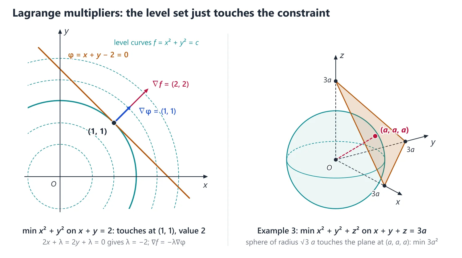
1. Understanding Limits in Two Variables
Why we need it: for a function of one variable, x can approach a only from the left or from the right. For a function f(x, y), such as the temperature on a metal plate, the point (x, y) can approach (a, b) from every direction and along every curve.
Continuity, partial derivatives and differentiability are all defined through this limit, so we must know exactly what it says before any of them can be tested.
In words: lim(x,y)→(a,b) f(x, y) = l means: whatever accuracy ε > 0 is demanded, there is a radius δ > 0 such that every point (x, y) of the disc of radius δ about (a, b), except (a, b) itself, gives a value f(x, y) within ε of l.
'For every ε' means the challenger chooses the accuracy; 'there is δ' means you answer with a disc; '0 < distance' means the value f(a, b) plays no part in the limit.
The disc contains points in every direction, so if the limit exists it is the same along every path into (a, b).
Continuity at (a, b) adds two requirements: f(a, b) is defined, and it equals the limit.
First example, slowly: we show that lim(x,y)→(0,0) x2y/(x2 + y2) = 0.
Step 1: guess the limit. On both axes the function is 0, so the only possible value is l = 0.
Step 2: put x = r cos θ, y = r sin θ. Then x2 + y2 = r2, and r is exactly the distance from the origin.
Step 3: the function becomes r3 cos2θ sin θ/r2 = r cos2θ sin θ.
Step 4: remove θ by a bound: |f − 0| = r|cos2θ sin θ| ≤ r, because |cos θ| ≤ 1 and |sin θ| ≤ 1.
Step 5: given ε > 0 choose δ = ε. If 0 < r < δ, then |f| ≤ r < ε.
Step 6: so the limit is 0. Notice that the bound r does not involve θ; one δ works for all directions at once, which is exactly what the definition demands.
Non-example: g(x, y) = x2/(x2 + y2) becomes cos2θ in polar form. It does not become small as r → 0: it is 1 on the x-axis and 0 on the y-axis.
The condition that fails is 'one δ for all directions': no disc about the origin keeps g within ε = 1/4 of a single number, so the limit does not exist.
Building up: four facts follow directly from the definition.
(1) Every path into (a, b) lies inside every disc about (a, b), so two paths with different limits prove that the limit does not exist.
(2) Agreement along all straight lines is not enough: x2y/(x4 + y2) tends to 0 along every line y = mx but equals 1/2 on the parabola y = x2.
(3) To prove that a limit exists, a bound |f − l| ≤ Krα with α > 0 and K free of θ always works, with δ = (ε/K)1/α.
(4) Continuity of f at (a, b) gives continuity of x ↦ f(x, b) and y ↦ f(a, y) (Standard Proofs, Theorem 14), but continuity in each variable separately does not give continuity of f.
Where it is used: every question 'examine the continuity (or differentiability) of f at (0, 0)' starts with this limit. The same ε–δ language returns in Real Analysis, and in Complex Analysis, where z → z0 also approaches from all directions.
2. Limits and Continuity
lim(x,y)→(a,b) f(x, y) = l if for every ε > 0 there is δ > 0 with 0 < √((x − a)2 + (y − b)2) < δ ⇒ |f(x, y) − l| < ε.
Idea: in the plane, (x, y) can approach (a, b) along infinitely many paths (lines, parabolas, spirals), not just from the left and the right, so a two-variable limit is a much stronger requirement than a one-variable one.
The limit must be the same along every path. To disprove existence, use paths such as y = mx or y = mx2; to prove existence, put x = r cos θ, y = r sin θ and bound |f − l| by a function of r alone that tends to 0.
Standard examples at (0, 0): xy/(x2 + y2) equals m/(1 + m2) along y = mx, which depends on m, so there is no limit; x2y/(x4 + y2) tends to 0 along every line y = mx but equals 1/2 along y = x2, so lines alone can never prove that a limit exists.
Equality of the repeated limits limx→a limy→b f and limy→b limx→a f does not imply that the double limit exists.
Choosing δ for a given ε: in polar coordinates bound |f(x, y) − l| ≤ Krα (α > 0), using |x| ≤ r and |y| ≤ r; then δ = (ε/K)1/α works.
If f(x, y) is continuous at (a, b), then x ↦ f(x, b) is continuous at a and y ↦ f(a, y) at b (proved in Standard Proofs); the converse is false.
3. Understanding Partial Derivatives and Differentiability
Why we need it: in one variable, a derivative at a point gives a tangent line, and it forces continuity. In two variables the partial derivatives look only along two lines through the point, so they guarantee neither.
We need a stronger notion, differentiability, which guarantees a tangent plane, continuity, the chain rule and Taylor's theorem.
In words: fx(a, b) is found by freezing y = b and differentiating the one-variable function x ↦ f(x, b) at x = a. Geometrically it is the slope of the curve cut from the surface z = f(x, y) by the plane y = b.
fy(a, b) is found in the same way with x frozen at a.
f is differentiable at (a, b) if f(a + h, b + k) − f(a, b) = Ah + Bk + ερ, where ρ = √(h2 + k2) and ε → 0 as (h, k) → (0, 0). Putting k = 0 and letting h → 0 shows that A = fx(a, b); similarly B = fy(a, b).
In plain terms: near the point, f equals a linear function plus an error that is small even when compared with the distance ρ from the point.
First example, slowly: take f(x, y) = x2 + 3xy at the point (1, 2).
Step 1: fx = 2x + 3y = 8 and fy = 3x = 3 at (1, 2), and f(1, 2) = 7.
Step 2: expand f(1 + h, 2 + k) = (1 + h)2 + 3(1 + h)(2 + k) = 7 + 8h + 3k + h2 + 3hk.
Step 3: the increment is 8h + 3k + (h2 + 3hk). The linear part has exactly the coefficients fx = 8 and fy = 3.
Step 4: the error is h2 + 3hk. Since |h| ≤ ρ and |k| ≤ ρ, its size is at most ρ2 + 3ρ2 = 4ρ2.
Step 5: so ε = (error)/ρ satisfies |ε| ≤ 4ρ → 0. Hence f is differentiable at (1, 2), with tangent plane z = 7 + 8(x − 1) + 3(y − 2).
Non-example: f = xy/√(x2 + y2), f(0, 0) = 0 (Worked Example 5 below) is continuous at the origin and has fx(0, 0) = fy(0, 0) = 0.
In polar form f = (r/2) sin 2θ, so along each ray the surface is a straight line: the graph is a cone-like surface over the origin. The error ratio hk/(h2 + k2) equals 1/2 along k = h, so it does not tend to 0, and there is no tangent plane.
Building up: the definition gives a chain of implications, and none of the arrows can be reversed.
(1) Differentiable ⇒ continuous, because the increment Ah + Bk + ερ tends to 0. (2) Differentiable ⇒ both partial derivatives exist (take k = 0, then h = 0).
(3) If fx, fy exist near the point and are continuous at it, then f is differentiable: this is the mean value argument in the line 'Why continuous partial derivatives suffice' below.
(4) The converses fail: xy/(x2 + y2) has partial derivatives but is not continuous; the non-example above is continuous but not differentiable; and f = (x2 + y2) sin(1/√(x2 + y2)), f(0, 0) = 0, is differentiable at the origin although fx is not continuous there.
(5) For mixed derivatives, fxy = fyx when the hypotheses of Schwarz's or Young's theorem hold (below); otherwise each must be computed from difference quotients.
Where it is used: differentiability is the hypothesis behind the chain rule, Euler's theorem, Taylor's theorem and tangent planes; UPSC regularly asks to test it at the origin for a function defined separately there.
4. Partial Derivatives and Differentiability
fx(a, b) = limh→0 (f(a + h, b) − f(a, b))/h, and similarly fy. Existence of the partial derivatives does not imply continuity.
Idea: fx looks only along the line y = b through the point, so it says nothing about other directions: xy/(x2 + y2) with value 0 at the origin has fx(0, 0) = fy(0, 0) = 0 (f vanishes on both axes) but is not even continuous there.
f is differentiable at (a, b) if f(a + h, b + k) − f(a, b) = hfx(a, b) + kfy(a, b) + ε√(h2 + k2) with ε → 0 as (h, k) → (0, 0). Differentiable ⇒ continuous; continuous partial derivatives near the point ⇒ differentiable.
Idea: differentiability means the surface z = f(x, y) has a genuine tangent plane z − f(a, b) = fx(a, b)(x − a) + fy(a, b)(y − b), with an error that is small compared with the distance √(h2 + k2).
Testing differentiability at a point (method): find fx, fy there from the definition, form ε(h, k) = (f(a + h, b + k) − f(a, b) − hfx − kfy)/√(h2 + k2), and check whether ε → 0 as (h, k) → (0, 0), using polar coordinates h = r cos θ, k = r sin θ.
Why continuous partial derivatives suffice: f(a + h, b + k) − f(a, b) = [f(a + h, b + k) − f(a, b + k)] + [f(a, b + k) − f(a, b)] = hfx(a + θ1h, b + k) + kfy(a, b + θ2k) by the MVT, and continuity of fx, fy at (a, b) makes these differ from hfx(a, b) + kfy(a, b) by a quantity small compared with √(h2 + k2).
Schwarz's theorem: if fx and fy exist near (a, b) and one mixed partial derivative exists near (a, b) and is continuous at (a, b), then the other mixed partial derivative exists at (a, b) and the two are equal. Young's theorem: if fx and fy are differentiable at (a, b), then fxy(a, b) = fyx(a, b).
Without these hypotheses the mixed derivatives can differ: for f = xy(x2 − y2)/(x2 + y2), f(0, 0) = 0, one finds fx(0, y) = −y and fy(x, 0) = x, so (fx)y(0, 0) = −1 while (fy)x(0, 0) = 1.
Euler's theorem: if f is homogeneous of degree n with continuous first partial derivatives, then xfx + yfy = nf; with continuous second derivatives, x2fxx + 2xyfxy + y2fyy = n(n − 1)f.
Proved in Standard Proofs, Theorem 13. Idea: differentiate f(tx, ty) = tnf(x, y) with respect to t and put t = 1.
Derivation of the second-order form: differentiating xfx + yfy = nf with respect to x and to y gives xfxx + yfxy = (n − 1)fx and xfxy + yfyy = (n − 1)fy (using fxy = fyx). Multiplying by x and y and adding: x2fxx + 2xyfxy + y2fyy = (n − 1)(xfx + yfy) = n(n − 1)f.
Chain rule: if z = f(x, y), x = x(t), y = y(t), then dz/dt = fx dx/dt + fy dy/dt. Taylor's theorem in two variables: f(a + h, b + k) = f(a, b) + (h∂/∂x + k∂/∂y)f + (1/2!)(h∂/∂x + k∂/∂y)2f + ..., derivatives evaluated at (a, b).
Why the chain rule needs differentiability: Δz = fxΔx + fyΔy + ε√(Δx2 + Δy2) with ε → 0; dividing by Δt and letting Δt → 0 removes the ε-term, since √(Δx2 + Δy2)/|Δt| stays bounded. If only the partial derivatives exist, the formula can fail.
Mixed derivatives at the origin (method): find fx(0, y) = limh→0 (f(h, y) − f(0, y))/h for y ≠ 0 and fx(0, 0) separately; then (fx)y(0, 0) = limk→0 (fx(0, k) − fx(0, 0))/k, and similarly in the other order. Books differ on whether fxy means (fx)y, so state your convention.
Euler's theorem for composite functions: if F(u) = z is homogeneous of degree n in x, y, then xux + yuy = nF(u)/F′(u) = g(u) and x2uxx + 2xyuxy + y2uyy = g(u)(g′(u) − 1). For a sum of homogeneous functions of different degrees, apply the theorem to each term and add.
Laplacian of rn: with r = √(x2 + y2 + z2), ∂2(rn)/∂x2 + ∂2(rn)/∂y2 + ∂2(rn)/∂z2 = n(n + 1)rn−2; in particular 1/r is harmonic for r ≠ 0.
5. Maxima and Minima
Stationary points: solve fx = fy = 0. Let r = fxx, s = fxy, t = fyy at the point.
rt − s2 > 0 and r < 0: maximum; rt − s2 > 0 and r > 0: minimum; rt − s2 < 0: saddle point; rt − s2 = 0: doubtful, examine further.
Derivation: at a stationary point Taylor's theorem gives f(a + h, b + k) − f(a, b) ≈ (1/2)(rh2 + 2shk + tk2), and for r ≠ 0, rh2 + 2shk + tk2 = [(rh + sk)2 + (rt − s2)k2]/r. If rt − s2 > 0 the bracket is positive for (h, k) ≠ (0, 0), so the difference has the sign of r; if rt − s2 < 0 the bracket is positive for k = 0 and negative when rh + sk = 0, so f increases in some directions and decreases in others.
Idea: a saddle point is a mountain pass, a maximum along one direction and a minimum along another, as for z = x2 − y2 at the origin.
For three variables use the Hessian H = [[fxx, fxy, fxz], [fyx, fyy, fyz], [fzx, fzy, fzz]]: a minimum if its leading principal minors are all positive, a maximum if they alternate in sign starting with a negative one.
When rt − s2 = 0: study f(a + h, b + k) − f(a, b) directly. Factorising it, or testing along curves (not only straight lines), may show a change of sign, and then there is no extremum.
6. Understanding Lagrange's Multipliers
Why we need it: many problems optimise a quantity while the variables are tied by a condition: the largest box with a given surface area, the nearest point of a surface to a given point. Solving the condition for one variable and substituting is often messy and destroys the symmetry of the problem.
Lagrange's method keeps all the variables on an equal footing.
In words: to find extreme values of f(x, y, z) on the surface φ(x, y, z) = 0, form F = f + λφ, where λ is an unknown number called the multiplier.
The equations Fx = Fy = Fz = 0 say ∇f = −λ∇φ: the gradient of f is parallel to the normal of the constraint surface.
Together with φ = 0 these are four equations in the four unknowns x, y, z, λ. Their solutions are only candidates; whether each is a maximum, a minimum or neither is decided afterwards.
First example, slowly: maximise f = xy subject to x + y = 10.
Step 1: write the constraint as φ = x + y − 10 = 0 and form F = xy + λ(x + y − 10).
Step 2: Fx = y + λ = 0 and Fy = x + λ = 0.
Step 3: subtracting the two equations eliminates λ and gives x = y.
Step 4: the constraint gives 2x = 10, so x = y = 5 (and λ = −5, which is not needed in the answer).
Step 5: on the line, f = x(10 − x) is a downward parabola, so the single candidate gives the maximum value f = 25.
Picture: the level curves xy = c are hyperbolas. As c grows they move away from the origin, and the last one that still meets the line x + y = 10 touches it at (5, 5); at a point of touching the two normals are parallel, which is the Lagrange condition.
Non-example: minimise f = x on the curve φ = y2 − x3 = 0. On the curve x3 = y2 ≥ 0, so x ≥ 0 and the minimum is at the origin.
But Fx = 1 − 3λx2 and Fy = 2λy have no common zero on the curve: y = 0 forces x = 0 and then Fx = 1, while λ = 0 also gives Fx = 1. The method misses the minimum because ∇φ = (−3x2, 2y) is 0 at the origin, so the hypothesis ∇φ ≠ 0 fails (the curve has a cusp there).
Building up: (1) at a constrained extremum P, every curve on the surface through P gives a function of one parameter with a stationary value at P, so ∇f · (tangent vector) = 0 at P.
(2) So ∇f is perpendicular to the whole tangent plane at P, hence parallel to the normal ∇φ, provided ∇φ ≠ 0. Writing ∇f = −λ∇φ gives Fx = Fy = Fz = 0 (derivation below).
(3) With two constraints the allowed directions form a single line, perpendicular to both ∇φ and ∇ψ; then ∇f lies in the plane of ∇φ and ∇ψ, which is why two multipliers appear.
(4) To decide the nature, use the geometry: a continuous function on a closed bounded constraint set attains a largest and a smallest value, so compare f at all candidates; or test the sign of d2F subject to dφ = 0.
Where it is used: the classical 15–20 mark question (extreme values on a central section of a conicoid, the largest box in an ellipsoid, the shortest distance to a curve or surface); in Analytic Geometry the same tangency gives normals and the semi-axes of central sections.
7. Lagrange's Method of Multipliers
To find the extrema of f(x, y, z) subject to φ(x, y, z) = 0: (1) form F = f + λφ; (2) solve Fx = Fy = Fz = 0 together with φ = 0; (3) decide the nature from the geometry of the problem or from the sign of d2F subject to dφ = 0.
Derivation: at a constrained extremum, df = fxdx + fydy + fzdz = 0 for every displacement tangent to the surface φ = 0, that is, for every (dx, dy, dz) with φxdx + φydy + φzdz = 0. So ∇f is perpendicular to the tangent plane of φ = 0 and hence parallel to its normal ∇φ ≠ 0: ∇f = −λ∇φ, which is exactly Fx = Fy = Fz = 0 for F = f + λφ.
Idea: at the extremum the level surface f = constant just touches the constraint surface; if it cut across, moving along the constraint would increase f on one side and decrease it on the other.
With two constraints φ = 0, ψ = 0 use F = f + λ1φ + λ2ψ. The method gives necessary conditions only, and requires ∇φ ≠ 0 (for two constraints, ∇φ and ∇ψ independent) at the point.
Two constraints on a central conicoid: for x2 + y2 + z2 subject to ax2 + by2 + cz2 = 1 and lx + my + nz = 0, multiplying Fx = 0, Fy = 0, Fz = 0 by x, y, z and adding gives λ1 = −u, and the stationary values u satisfy l2/(1 − au) + m2/(1 − bu) + n2/(1 − cu) = 0.
The nearest and farthest points of a sphere from an outside point lie on the line through that point and the centre; Lagrange's equations confirm this.
8. Understanding Jacobians
Why we need it: when we change variables from (x, y) to (u, v), three questions arise: how do small areas change (needed in double integrals), can the change be undone, and do u and v carry independent information? One determinant answers all three.
In words: ∂(u, v)/∂(x, y) is the determinant of the 2 × 2 matrix whose first row (ux, uy) says how u changes with x and y, and whose second row (vx, vy) says the same for v.
Its absolute value is the factor by which a tiny area in the xy-plane is multiplied when it is carried to the uv-plane; its sign tells whether the orientation is kept (+) or reversed (−).
A zero Jacobian means the two rows, the gradients ∇u and ∇v, are parallel: u and v increase in the same direction, so they are not independent.
First example, slowly: take u = x + y, v = x − y.
Step 1: ux = 1, uy = 1, vx = 1, vy = −1.
Step 2: ∂(u, v)/∂(x, y) = (1)(−1) − (1)(1) = −2.
Step 3: check the meaning of |J| = 2. The unit square with corners (0, 0), (1, 0), (0, 1), (1, 1) goes to the square with corners (0, 0), (1, 1), (1, −1), (2, 0), whose side is √2 and area 2.
Step 4: the negative sign says the map reverses orientation, like a reflection.
Step 5: the inverse map is x = (u + v)/2, y = (u − v)/2, with ∂(x, y)/∂(u, v) = (1/2)(−1/2) − (1/2)(1/2) = −1/2, and (−2)(−1/2) = 1, as the inverse rule says.
Non-example: u = x + y, v = (x + y)2 gives J = 1·2(x + y) − 1·2(x + y) = 0 everywhere. This pair cannot serve as new coordinates: every point (x, y) goes to the parabola v = u2, many points go to the same (u, v), and no inverse exists. The condition J ≠ 0 is what fails.
Building up: (1) the linear map x = au + bv, y = cu + dv sends the unit square to a parallelogram of area |ad − bc|, the absolute value of its determinant.
(2) A differentiable map is almost linear on a tiny rectangle, with the matrix of partial derivatives as its linear part, so locally the area factor is |J|.
(3) The chain rule ∂(u, v)/∂(r, s) = ∂(u, v)/∂(x, y)·∂(x, y)/∂(r, s) and the inverse rule follow from det(AB) = det A·det B, because the matrix of a composite map is the product of the matrices.
(4) If J ≡ 0 in a region, ∇u and ∇v are parallel everywhere, the level curves of u and v coincide, and v is a function of u near every point where ∇u ≠ 0.
(5) If u, v have continuous partial derivatives and J ≠ 0 at a point, the inverse function theorem says the map can be inverted near that point.
Where it is used: dx dy = |∂(x, y)/∂(u, v)| du dv in the next topic, and questions on functional dependence (Worked Example 4 and the Jacobian questions among the Solved UPSC Questions below).
9. Jacobians
J = ∂(u, v)/∂(x, y) = det[[ux, uy], [vx, vy]]. Chain rule: ∂(u, v)/∂(r, s) = ∂(u, v)/∂(x, y) · ∂(x, y)/∂(r, s); inverse rule: ∂(u, v)/∂(x, y) · ∂(x, y)/∂(u, v) = 1.
Idea: the Jacobian is the local area (or volume) magnification factor of the map (x, y) ↦ (u, v): a small rectangle of area dx dy goes to a small parallelogram of area |J| dx dy, and the sign of J tells whether orientation is kept. The chain and inverse rules are det(AB) = det A·det B applied to the matrices of partial derivatives.
Functional dependence: u and v (with continuous partial derivatives) are functionally related if and only if ∂(u, v)/∂(x, y) = 0 identically in the region (the 'if' part holds locally, near points where ux and uy do not both vanish).
Idea: if v = φ(u), the level curves of u and v coincide, so ∇u and ∇v are parallel and the determinant of their components vanishes; for u = x + y, v = (x + y)2, J = 1·2(x + y) − 1·2(x + y) = 0.
Standard values: ∂(x, y)/∂(r, θ) = r (polar); ∂(x, y, z)/∂(r, θ, z) = r (cylindrical); ∂(x, y, z)/∂(r, θ, φ) = r2 sin θ (spherical).
Derivation: x = r cos θ, y = r sin θ gives ∂(x, y)/∂(r, θ) = det[[cos θ, −r sin θ], [sin θ, r cos θ]] = r cos2θ + r sin2θ = r; the spherical value is derived in the next topic.
Finding the relation: once ∂(u, v)/∂(x, y) = 0, eliminate the variables, or put one variable equal to a convenient constant (often 0) in u = φ(v) to identify φ.
10. Choosing the Method
If the function is homogeneous, or a function of a homogeneous expression → Euler's theorem (or its composite form) instead of computing the derivatives.
If variables are changed (x, y in terms of r, θ or u, v) → chain rule; write the full chain before substituting.
If the extremum is free → stationary points and rt − s2; if there are constraints → Lagrange multipliers, or substitution when the constraint is easily solved for one variable. The second table of this topic summarises the standard problems.
11. Common Mistakes
Claiming that a limit exists because it is the same along every line y = mx.
Writing 'the partial derivatives exist, so f is differentiable' (or continuous); both implications are false.
Computing fxy(0, 0) by differentiating the formula valid for (x, y) ≠ (0, 0) and then substituting (0, 0); at the origin use difference quotients.
Evaluating r, s, t as general expressions instead of at each stationary point, or declaring 'no extremum' when rt − s2 = 0.
In Lagrange problems, stopping at the values of λ or missing some solutions of the system; λ is auxiliary, and every solution must be checked.
Using the Jacobian the wrong way round: dx dy = |∂(x, y)/∂(u, v)| du dv, not |∂(u, v)/∂(x, y)| du dv.
12. Connections
Link: ∇f, the tangent plane and the normal to a surface φ = 0 lead directly to the gradient and directional derivative of Vector Analysis and to tangent planes of conicoids (Analytic Geometry).
Link: Jacobians are the change-of-variables factor in double and triple integrals (next topic), and the Hessian test is the positive-definiteness test for symmetric matrices (Linear Algebra).
Link: f = u + iv is complex differentiable when u, v are differentiable with ux = vy, uy = −vx, and then ∂(u, v)/∂(x, y) = ux2 + vx2 = |f′(z)|2 (Complex Analysis).
13. Worked Examples
Example 1: Show that lim(x,y)→(0,0) xy/(x2 + y2) does not exist. Along y = mx the value is m/(1 + m2), which depends on m.
Example 2: Find the extreme values of f = x3 + y3 − 3axy (a > 0).
fx = 3x2 − 3ay = 0 and fy = 3y2 − 3ax = 0 give (0, 0) and (a, a). At (0, 0): r = t = 0, s = −3a, rt − s2 < 0, a saddle point. At (a, a): r = 6a > 0 and rt − s2 = 36a2 − 9a2 > 0, a minimum with value −a3.
Example 3: Find the minimum of x2 + y2 + z2 subject to x + y + z = 3a.
F = x2 + y2 + z2 + λ(x + y + z − 3a); 2x + λ = 2y + λ = 2z + λ = 0 gives x = y = z = a, and the minimum value is 3a2 (the square of the distance from the origin to the plane).
Example 4: If u = x + y + z, v = xy + yz + zx and w = x2 + y2 + z2, then ∂(u, v, w)/∂(x, y, z) = 0, because w = u2 − 2v: u, v, w are functionally dependent.
Example 5: Let f(x, y) = xy/√(x2 + y2) for (x, y) ≠ (0, 0) and f(0, 0) = 0. Show that f is continuous at (0, 0) and has partial derivatives there, but is not differentiable at (0, 0).
Since |xy| ≤ (x2 + y2)/2, |f(x, y)| ≤ √(x2 + y2)/2 → 0, so f is continuous at (0, 0).
f(h, 0) = 0 = f(0, k), so fx(0, 0) = fy(0, 0) = 0.
If f were differentiable, then (f(h, k) − 0 − 0·h − 0·k)/ρ → 0 with ρ = √(h2 + k2). But this ratio is hk/(h2 + k2), which equals 1/2 along k = h. So f is not differentiable at (0, 0).
Example 6: If u = sin−1((x2 + y2)/(x + y)), show that xux + yuy = tan u and x2uxx + 2xyuxy + y2uyy = tan3u.
z = sin u = (x2 + y2)/(x + y) is homogeneous of degree 1, so by Euler's theorem xzx + yzy = z.
Since zx = cos u·ux and zy = cos u·uy: cos u (xux + yuy) = sin u, so xux + yuy = tan u = g(u).
Differentiating xux + yuy = g(u) w.r.t. x and y, multiplying by x and y and adding gives x2uxx + 2xyuxy + y2uyy = g(u)(g′(u) − 1) = tan u (sec2u − 1) = tan3u.
14. Solved UPSC Questions
Example 7 (UPSC 2014, 20 marks): Find the maximum or minimum values of x2 + y2 + z2 subject to the conditions ax2 + by2 + cz2 = 1 and lx + my + nz = 0. Interpret the result geometrically.
F = x2 + y2 + z2 + λ1(ax2 + by2 + cz2 − 1) + λ2(lx + my + nz). Fx = 0 gives 2x + 2λ1ax + λ2l = 0, and similarly 2y + 2λ1by + λ2m = 0, 2z + 2λ1cz + λ2n = 0.
Multiply by x, y, z and add, using both constraints: 2u + 2λ1 = 0, where u = x2 + y2 + z2 is the stationary value. So λ1 = −u.
Then 2x(1 − au) = −λ2l, so x = −λ2l/(2(1 − au)), y = −λ2m/(2(1 − bu)), z = −λ2n/(2(1 − cu)) (in the generic case 1 − au, 1 − bu, 1 − cu ≠ 0, and λ2 ≠ 0 since (x, y, z) ≠ 0).
Substituting into lx + my + nz = 0: l2/(1 − au) + m2/(1 − bu) + n2/(1 − cu) = 0, a quadratic in u (after clearing denominators) whose two roots are the maximum and minimum values.
Interpretation: ax2 + by2 + cz2 = 1 is a central conicoid and lx + my + nz = 0 a plane through its centre. Their section is a central conic, and x2 + y2 + z2 is the squared distance from the centre, so the two roots are the squares of the semi-axes of this section.
Answer: The extreme values u are the roots of l2/(1 − au) + m2/(1 − bu) + n2/(1 − cu) = 0; they are the squares of the semi-axes of the central section.
Example 8 (UPSC 2016, 20 marks): Find the maximum and minimum values of x2 + y2 + z2 subject to the conditions x2/4 + y2/5 + z2/25 = 1 and x + y − z = 0.
This is the previous example with a = 1/4, b = 1/5, c = 1/25 and l = m = 1, n = −1. The stationary values u satisfy 4/(4 − u) + 5/(5 − u) + 25/(25 − u) = 0.
Clearing denominators: 4(5 − u)(25 − u) + 5(4 − u)(25 − u) + 25(4 − u)(5 − u) = (500 − 120u + 4u2) + (500 − 145u + 5u2) + (500 − 225u + 25u2) = 0.
So 34u2 − 490u + 1500 = 0, i.e. 17u2 − 245u + 750 = 0, with discriminant 2452 − 51000 = 9025 = 952 and roots u = (245 ± 95)/34 = 10, 75/17.
Both are attained: the plane x + y = z cuts the ellipsoid in an ellipse with semi-axes √10 and √(75/17).
Answer: Maximum 10, minimum 75/17.
Example 9 (UPSC 2015, 13 marks): Which point of the sphere x2 + y2 + z2 = 1 is at the maximum distance from the point (2, 1, 3)?
Maximise D = (x − 2)2 + (y − 1)2 + (z − 3)2 subject to x2 + y2 + z2 = 1, with F = D + λ(x2 + y2 + z2 − 1).
Fx = 2(x − 2) + 2λx = 0 gives x = 2/(1 + λ); similarly y = 1/(1 + λ), z = 3/(1 + λ). So (x, y, z) = t(2, 1, 3) with t = 1/(1 + λ).
The constraint gives 14t2 = 1, t = ±1/√14. The distance is |1 − t|√14: √14 − 1 for t = 1/√14 (nearest) and √14 + 1 for t = −1/√14 (farthest).
Answer: The point (−2/√14, −1/√14, −3/√14), at distance √14 + 1.
Example 10 (UPSC 2015, 12 marks): For the function f(x, y) = (x2 − x√y)/(x2 + y), (x, y) ≠ (0, 0); f(x, y) = 0, (x, y) = (0, 0), examine the continuity and differentiability.
√y requires y ≥ 0, so f is defined on the closed upper half-plane (except where x2 + y = 0, i.e. the origin, where f = 0 by definition).
Along y = 0 (x ≠ 0): f(x, 0) = x2/x2 = 1 → 1. Along x = 0 (y > 0): f(0, y) = 0 → 0.
The limits along two paths differ, so lim(x,y)→(0,0) f does not exist: f is discontinuous at (0, 0), and therefore not differentiable there. (Even fx(0, 0) = lim (f(h, 0) − 0)/h = lim 1/h fails to exist.)
At every other point with y > 0, f is a quotient of functions with continuous partial derivatives and non-zero denominator, hence continuous and differentiable.
Answer: f is neither continuous nor differentiable at (0, 0); it is both at the other points with y > 0.
Example 11 (UPSC 2017, 15 marks): If f(x, y) = xy(x2 − y2)/(x2 + y2), (x, y) ≠ (0, 0);
f(x, y) = 0, (x, y) = (0, 0),
calculate ∂2f/∂x∂y and ∂2f/∂y∂x at (0, 0).
Convention: ∂2f/∂x∂y = ∂/∂x(∂f/∂y) and ∂2f/∂y∂x = ∂/∂y(∂f/∂x).
For y ≠ 0: fx(0, y) = limh→0 f(h, y)/h = lim y(h2 − y2)/(h2 + y2) = −y; and fx(0, 0) = lim f(h, 0)/h = 0. So fx(0, y) = −y for all y.
For x ≠ 0: fy(x, 0) = limk→0 f(x, k)/k = lim x(x2 − k2)/(x2 + k2) = x; and fy(0, 0) = 0. So fy(x, 0) = x for all x.
∂2f/∂y∂x (0, 0) = limk→0 (fx(0, k) − fx(0, 0))/k = −1, and ∂2f/∂x∂y (0, 0) = limh→0 (fy(h, 0) − fy(0, 0))/h = 1.
The two are unequal; Schwarz's theorem does not apply because the mixed partial derivatives are not continuous at (0, 0).
Answer: ∂2f/∂x∂y (0, 0) = 1 and ∂2f/∂y∂x (0, 0) = −1.
Example 12 (UPSC 2025, 15 marks): If f(x, y) = xy (x2 − y2)/(x2 + y2), when (x, y) ≠ (0, 0)
f(x, y) = 0, when (x, y) = (0, 0),
then find fxy(0, 0) and fyx(0, 0).
This is the function of the previous example. From first principles, fx(0, y) = −y for all y and fy(x, 0) = x for all x.
With fxy = (fx)y: fxy(0, 0) = limk→0 (fx(0, k) − fx(0, 0))/k = lim (−k)/k = −1.
fyx = (fy)x: fyx(0, 0) = limh→0 (fy(h, 0) − fy(0, 0))/h = lim h/h = 1. (With the opposite convention the two values are interchanged; state the convention in the answer.)
Answer: fxy(0, 0) = −1, fyx(0, 0) = 1, so fxy(0, 0) ≠ fyx(0, 0).
Example 13 (UPSC 2018, 13 marks): Find the shortest distance from the point (1, 0) to the parabola y2 = 4x.
Minimise D = (x − 1)2 + y2 subject to y2 = 4x (so x ≥ 0), with F = (x − 1)2 + y2 + λ(y2 − 4x).
Fx = 2(x − 1) − 4λ = 0 and Fy = 2y(1 + λ) = 0. If λ = −1 then x = −1, impossible since y2 = 4x ≥ 0; so y = 0 and x = 0.
Check directly: on the parabola D = (x − 1)2 + 4x = (x + 1)2, which for x ≥ 0 is least at x = 0. (The point (1, 0) is the focus, and the vertex is the nearest point.)
Answer: Shortest distance 1, attained at the vertex (0, 0).
Example 14 (UPSC 2018, 12 marks): Let
f(x, y) = xy2, if y > 0
= −xy2, if y ≤ 0.
Determine which of ∂f/∂x (0, 1) and ∂f/∂y (0, 1) exists and which does not exist.
For all (x, y), f(x, y) = xy|y| (for y ≤ 0, xy|y| = −xy2). Near (0, 1), y > 0, so f = xy2 there.
∂f/∂x (0, 1) = limh→0 (f(h, 1) − f(0, 1))/h = lim (h − 0)/h = 1, so it exists.
∂f/∂y (0, 1) = limk→0 (f(0, 1 + k) − f(0, 1))/k = lim (0 − 0)/k = 0, so it also exists.
In fact fx = y|y| and fy = 2x|y| exist at every point, even on y = 0 where the formula changes, because t|t| is differentiable with derivative 2|t|.
Answer: Both exist: ∂f/∂x (0, 1) = 1 and ∂f/∂y (0, 1) = 0.
Example 15 (UPSC 2019, 20 marks): (i) If
u = sin−1 √((x1/3 + y1/3)/(x1/2 + y1/2))
then show that sin2u is a homogeneous function of x and y of degree −1/6. Hence show that
x2 ∂2u/∂x2 + 2xy ∂2u/∂x∂y + y2 ∂2u/∂y2 = (tan u/12)(13/12 + tan2u/12) (12 marks)
(ii) Using the Jacobian method, show that if f′(x) = 1/(1 + x2) and f(0) = 0, then
f(x) + f(y) = f((x + y)/(1 − xy)) (8 marks)
(i) z = sin2u = (x1/3 + y1/3)/(x1/2 + y1/2); replacing x, y by tx, ty multiplies it by t1/3/t1/2 = t−1/6, so z is homogeneous of degree −1/6.
Euler: xzx + yzy = −z/6. Since zx = 2 sin u cos u · ux (similarly for y), 2 sin u cos u (xux + yuy) = −sin2u/6, so xux + yuy = −tan u/12 = g(u).
Differentiating xux + yuy = g(u) w.r.t. x and y, multiplying by x and y and adding: x2uxx + 2xyuxy + y2uyy = g(u)(g′(u) − 1) = (−tan u/12)(−sec2u/12 − 1) = (tan u/12)(1 + (1 + tan2u)/12) = (tan u/12)(13/12 + tan2u/12).
(ii) Let u = f(x) + f(y), v = (x + y)/(1 − xy). Then ux = 1/(1 + x2), uy = 1/(1 + y2), vx = (1 + y2)/(1 − xy)2, vy = (1 + x2)/(1 − xy)2.
∂(u, v)/∂(x, y) = uxvy − uyvx = 1/(1 − xy)2 − 1/(1 − xy)2 = 0, so u and v are functionally related: u = φ(v).
Put y = 0: f(x) + f(0) = φ(x), i.e. φ = f since f(0) = 0. Hence f(x) + f(y) = f((x + y)/(1 − xy)).
Answer: Both identities hold as shown (f is in fact tan−1x).
Example 16 (UPSC 2024, 15 marks): If u = (x + y)/(1 − xy) and v = tan−1 x + tan−1 y, then find ∂(u, v)/∂(x, y). Are u and v functionally related? If yes, find the relationship.
ux = (1 + y2)/(1 − xy)2, uy = (1 + x2)/(1 − xy)2, vx = 1/(1 + x2), vy = 1/(1 + y2).
∂(u, v)/∂(x, y) = uxvy − uyvx = 1/(1 − xy)2 − 1/(1 − xy)2 = 0 (for xy ≠ 1), so u and v are functionally related.
The relation: tan v = tan(tan−1x + tan−1y) = (x + y)/(1 − xy) = u.
Answer: ∂(u, v)/∂(x, y) = 0; yes, u = tan v.
Example 17 (UPSC 2021, 15 marks): Given that f(x, y) = |x2 − y2|. Find fxy(0, 0) and fyx(0, 0). Hence show that fxy(0, 0) = fyx(0, 0).
For y ≠ 0 and |h| < |y|, |h2 − y2| = y2 − h2, so fx(0, y) = limh→0 (y2 − h2 − y2)/h = lim (−h) = 0. At y = 0, fx(0, 0) = lim h2/h = 0. So fx(0, y) = 0 for all y.
Hence fxy(0, 0) = limk→0 (fx(0, k) − fx(0, 0))/k = 0.
f(x, y) = f(y, x), so in the same way fy(x, 0) = 0 for all x and fyx(0, 0) = limh→0 (fy(h, 0) − fy(0, 0))/h = 0.
Answer: fxy(0, 0) = fyx(0, 0) = 0.
Example 18 (UPSC 2022, 15 marks): A wire of length l is cut into two parts which are bent in the form of a square and a circle respectively. Using Lagrange's method of undetermined multipliers, find the least value of the sum of the areas so formed.
Let the square have side a and the circle radius r. The constraint is 4a + 2πr = l and the total area is A = a2 + πr2.
F = a2 + πr2 + λ(4a + 2πr − l): Fa = 2a + 4λ = 0 and Fr = 2πr + 2πλ = 0 give a = −2λ, r = −λ, so a = 2r.
Then 8r + 2πr = l, so r = l/(2(π + 4)) and a = l/(π + 4). A = l2/(π + 4)2 + πl2/(4(π + 4)2) = l2(4 + π)/(4(π + 4)2) = l2/(4(π + 4)).
This is the minimum: on the constraint line A is a convex quadratic, and the end values l2/16 (all square) and l2/(4π) (all circle) are both larger.
Answer: Least total area l2/(4(π + 4)), when the side of the square equals the diameter of the circle.
Example 19 (UPSC 2023, 15 marks): Justify whether (0, 0) is an extreme point for the function f(x, y) = 2x4 − 3x2y + y2.
fx = 8x3 − 6xy and fy = −3x2 + 2y vanish at (0, 0). There r = 24x2 − 6y = 0, s = −6x = 0, t = 2, so rt − s2 = 0 and the test is inconclusive.
Factorise: f(x, y) = (2x2 − y)(x2 − y), and f(0, 0) = 0.
On the y-axis, f(0, y) = y2 > 0 (y ≠ 0). On the parabola y = (3/2)x2, which lies between y = x2 and y = 2x2, f = (x2/2)(−x2/2) = −x4/4 < 0 (x ≠ 0).
So every neighbourhood of (0, 0) has points with f > 0 and points with f < 0. (Along every straight line through the origin f has a minimum at O, which shows that testing lines alone is not enough.)
Answer: (0, 0) is a stationary point but not an extreme point of f.
Example 20 (UPSC 2026, 10 marks): If u(x, y, z) = (x2 + y2 + z2)−1/2, then find the value of ∂2u/∂x2 + ∂2u/∂y2 + ∂2u/∂z2.
Let r = √(x2 + y2 + z2), so u = r−1 and ∂r/∂x = x/r. Then ux = −r−2(x/r) = −xr−3.
uxx = −r−3 + 3xr−4(x/r) = −r−3 + 3x2r−5; similarly uyy = −r−3 + 3y2r−5 and uzz = −r−3 + 3z2r−5.
Adding: −3r−3 + 3(x2 + y2 + z2)r−5 = −3r−3 + 3r−3 = 0.
Answer: 0 at every point other than the origin (u = 1/r satisfies Laplace's equation).
15. Practice Exercises
Exercise 1 (basic): Show that lim(x,y)→(0,0) (x2 − y2)/(x2 + y2) does not exist.
Answer: along y = mx the value is (1 − m2)/(1 + m2), which depends on m (it is 1 on the x-axis and −1 on the y-axis).
Exercise 2 (basic): For f(x, y) = x3y + exy, find fx(1, 0) and fy(1, 0).
Answer: fx = 3x2y + yexy = 0 and fy = x3 + xexy = 2 at (1, 0).
Exercise 3 (basic): Find ∂(u, v)/∂(x, y) for u = x2 − y2, v = 2xy.
Answer: det [[2x, −2y], [2y, 2x]] = 4(x2 + y2).
Exercise 4 (standard): Let f(x, y) = (x3 − y3)/(x2 + y2) for (x, y) ≠ (0, 0) and f(0, 0) = 0. Show that f is continuous at (0, 0), find fx(0, 0) and fy(0, 0), and decide whether f is differentiable at (0, 0).
Answer: |f| ≤ 2r, so f is continuous; fx(0, 0) = 1, fy(0, 0) = −1. The ratio (f(h, k) − h + k)/ρ equals (cos θ − sin θ) sin θ cos θ, which is −1/√2 for θ = −π/4 and does not tend to 0, so f is not differentiable at (0, 0).
Exercise 5 (standard): If u = tan−1((x3 + y3)/(x − y)), show that xux + yuy = sin 2u.
Answer: tan u is homogeneous of degree 2, so by Euler's theorem for composite functions xux + yuy = 2 tan u/sec2u = 2 sin u cos u = sin 2u.
Exercise 6 (standard): Find and classify the stationary points of f(x, y) = x2 + xy + y2 − 3x − 6y.
Answer: only (0, 3); r = 2, s = 1, t = 2, rt − s2 = 3 > 0 and r > 0, so a minimum, with value −9.
Exercise 7 (standard): Using Lagrange's method, find the maximum of xyz for positive x, y, z with x + y + z = 12.
Answer: yz = xz = xy = −λ gives x = y = z = 4; the maximum is 64 (xyz → 0 on the boundary of the triangle).
Exercise 8 (UPSC level): Find the volume of the largest rectangular parallelepiped, with edges parallel to the axes, that can be inscribed in the ellipsoid x2/a2 + y2/b2 + z2/c2 = 1.
Answer: with V = 8xyz and F = 8xyz + λ(x2/a2 + y2/b2 + z2/c2 − 1), multiplying Fx = 0, Fy = 0, Fz = 0 by x, y, z gives x2/a2 = y2/b2 = z2/c2 = 1/3; the maximum volume is 8abc/(3√3).
Exercise 9 (UPSC level): Examine f(x, y) = x4 + y4 − 2x2 + 4xy − 2y2 for maxima and minima.
Answer: stationary points (0, 0), (√2, −√2), (−√2, √2). At the last two r = t = 20, s = 4, so minima with value −8. At (0, 0), rt − s2 = 0; f(x, 0) = x4 − 2x2 < 0 and f(x, x) = 2x4 > 0 for small x ≠ 0, so there is no extremum.
Exercise 10 (UPSC level): If u = x + y + z, v = x2 + y2 + z2 − 2xy − 2yz − 2zx and w = x3 + y3 + z3 − 3xyz, show that u, v, w are functionally dependent and find the relation.
Answer: ∂(u, v, w)/∂(x, y, z) = 0. With s = x2 + y2 + z2 and p = xy + yz + zx: u2 = s + 2p, v = s − 2p and w = u(s − p), which give 4w = u3 + 3uv.
| Transformation | Equations | Jacobian |
|---|---|---|
| Plane polar | x = r cos θ, y = r sin θ | ∂(x, y)/∂(r, θ) = r |
| Elliptic polar | x = ar cos θ, y = br sin θ | abr |
| Linear | x = au + bv, y = cu + dv | ad − bc |
| Cylindrical | x = r cos θ, y = r sin θ, z = z | r |
| Spherical | x = r sin θ cos φ, y = r sin θ sin φ, z = r cos θ | r2 sin θ |
| Problem | Method | Watch out for |
|---|---|---|
| Does the limit exist at (0, 0)? | Disprove: two paths (y = mx, y = mx2, an axis) with different limits. Prove: polar form and a bound Krα | Lines alone never prove existence |
| Continuity at a point | Find the limit as above and compare with f(a, b) | f(a, b) is often defined separately |
| Differentiability at a point | fx, fy from the definition, then test ε(h, k) → 0 | Existence of the partial derivatives is not enough |
| Is fxy = fyx at (0, 0)? | fx(0, k), fy(h, 0) from the definition, then difference quotients | State which order fxy means |
| Free extrema | fx = fy = 0, then rt − s2 (Hessian minors for three variables) | rt − s2 = 0 needs direct study |
| Extrema with constraints | Lagrange multipliers, or substitution | Need ∇φ ≠ 0; find and test all solutions |
| Functional dependence | Show ∂(u, v)/∂(x, y) ≡ 0, then find the relation | J must vanish identically, not at one point |
Mains points
- Very frequent: Lagrange's multipliers for a geometric optimisation (largest box in an ellipsoid, shortest distance from a point to a surface); show the λ-equations, solve them symmetrically, and state the nature.
- Standard question: show that f has partial derivatives at (0, 0) but is not continuous or not differentiable there; compute fx(0, 0) and fy(0, 0) from the definition, not from formulas.
- Show fxy(0, 0) ≠ fyx(0, 0) for functions such as xy(x2 − y2)/(x2 + y2); use the limit definition of each mixed derivative.
- For unconstrained extrema, list every stationary point and classify each one; missing a stationary point is the most common loss of marks.
- Jacobian questions: verify JJ′ = 1, or test functional dependence and find the relation.
Did you know?
- For xy(x2 − y2)/(x2 + y2) with f(0, 0) = 0, fxy(0, 0) = −1 and fyx(0, 0) = 1 (with fxy meaning ∂/∂y of fx), the classic proof that mixed partial derivatives need not be equal.
Riemann Integral, Indefinite Integrals and Improper Integrals
A bounded function is Riemann integrable when its upper and lower integrals agree, equivalently when U(P, f) − L(P, f) can be made less than any ε. Definite integrals can be computed as limits of sums and through the fundamental theorem of calculus. Improper integrals (infinite range or unbounded integrand) are tested by p-tests, comparison and Dirichlet's test, and many are evaluated through Beta and Gamma functions.
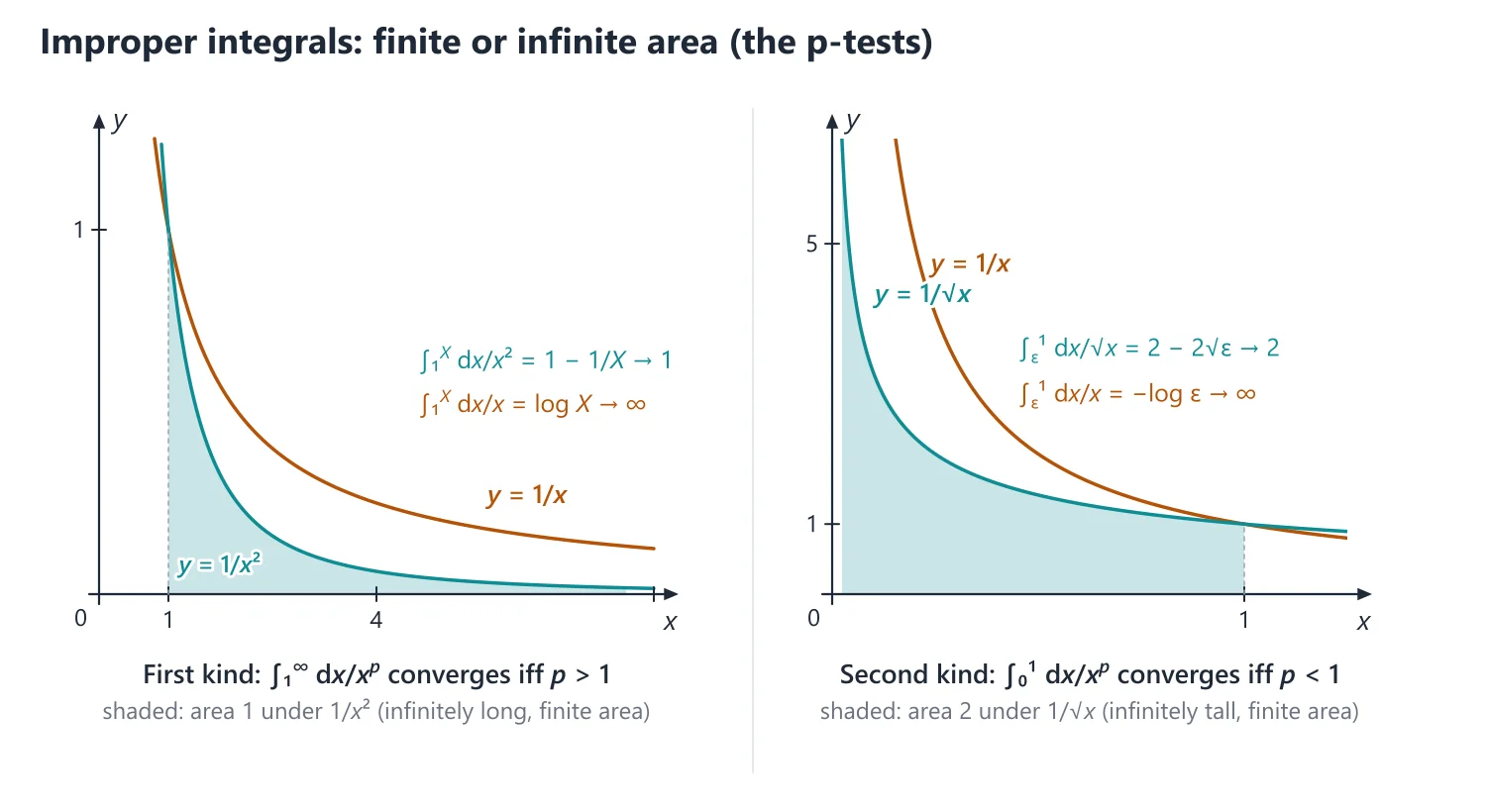
1. Understanding Upper and Lower Sums
Why we need it: 'the area under a curve' is easy to imagine but must be defined before it can be computed. We also need to know which functions have an integral at all, because a function that jumps wildly may not.
Riemann's idea is to trap the area between a sum of rectangles drawn from above and a sum drawn from below.
In words: a partition P cuts [a, b] into pieces at the points a = x0 < x1 < ... < xn = b. On the i-th piece, Mi is the supremum (the top of f there) and mi the infimum (the bottom).
U(P, f) = ∑MiΔxi over-estimates the area and L(P, f) = ∑miΔxi under-estimates it.
The upper integral is the best (smallest) over-estimate over all partitions, and the lower integral the best (largest) under-estimate. f is integrable when these two best estimates meet.
f must be bounded, so that every Mi and mi is a finite number.
First example, slowly: f(x) = x2 on [0, 1], with the partition Pn into n equal parts.
Step 1: the points are xi = i/n, and every Δxi = 1/n.
Step 2: x2 is increasing on [0, 1], so on each piece the top is at the right end and the bottom at the left end: Mi = (i/n)2, mi = ((i − 1)/n)2.
Step 3: U = (1/n3)(12 + 22 + ... + n2) = n(n + 1)(2n + 1)/(6n3).
Step 4: L = (1/n3)(02 + 12 + ... + (n − 1)2) = (n − 1)n(2n − 1)/(6n3).
Step 5: U − L = n2/n3 = 1/n → 0, and both U and L tend to 2/6 = 1/3.
Step 6: the upper integral is at most every U and the lower integral at least every L, so both equal 1/3: ∫01 x2 dx = 1/3.
Non-example: the Dirichlet function (1 on rationals, 0 on irrationals) on [0, 1] is bounded, but every piece of every partition contains both kinds of numbers, so every Mi = 1 and mi = 0.
Then U = 1 and L = 0 for every P, the upper integral is 1 and the lower integral 0. The condition that fails is that U − L can be made small; f is discontinuous at every point.
Building up: (1) adding points to a partition can only lower U and raise L (the refinement line below).
(2) Hence every lower sum is at most every upper sum: compare both with their common refinement.
(3) So L(P, f) ≤ lower integral ≤ upper integral ≤ U(P, f) for every P, and Riemann's criterion follows: f is integrable if and only if U − L can be made less than any ε > 0.
(4) For continuous f, uniform continuity makes Mi − mi small on short pieces, so U − L → 0 (Standard Proofs, Theorem 11); for monotonic f the differences telescope.
(5) Changing f at finitely many points changes neither integrability nor the value of the integral, because those points can be enclosed in pieces of total length as small as we like.
Where it is used: questions that say 'show from the definition' or 'by upper and lower sums', integrability of piecewise functions, and the trapezoidal and Simpson's rules of Numerical Analysis, which are refined versions of these sums.
2. Understanding the Integral as a Limit of Sums and the Fundamental Theorem
Why we need it: upper and lower sums define the integral, but finding suprema for every partition is slow. Two shortcuts do the real work: if f is known to be integrable, any convenient sequence of sums gives the integral; and if f has an antiderivative F, the integral is F(b) − F(a).
Read backwards, the first shortcut turns certain limits of sums into integrals.
In words: a Riemann sum S = ∑f(ti)Δxi uses any point ti of the i-th piece. Since mi ≤ f(ti) ≤ Mi, every Riemann sum lies between L(P, f) and U(P, f).
With n equal parts and right end points, S = ((b − a)/n)∑r=1n f(a + r(b − a)/n); on [0, 1] this is (1/n)∑f(r/n), where r/n plays the role of x and 1/n the role of dx.
The fundamental theorem says that F(x) = ∫ax f(t) dt, the area accumulated up to x, has derivative f(x) wherever f is continuous.
First example, slowly: find limn→∞ (1/(n + 1) + 1/(n + 2) + ... + 1/(2n)).
Step 1: the general term is 1/(n + r), for r = 1, 2, ..., n.
Step 2: take out 1/n: 1/(n + r) = (1/n)·1/(1 + r/n).
Step 3: so the sum is (1/n)∑f(r/n) with f(x) = 1/(1 + x), a Riemann sum on [0, 1].
Step 4: f is continuous on [0, 1], hence integrable, so the sum tends to ∫01 dx/(1 + x).
Step 5: an antiderivative is log(1 + x), so by the fundamental theorem the limit is log 2 − log 1 = log 2 ≈ 0.693.
Non-example: ∑r=1n 1/(n2 + r) looks similar, but its general term cannot be written as (1/n)f(r/n) with f independent of n, so it is not a Riemann sum.
Here a direct bound works instead: each term is at most 1/n2, so the sum is at most 1/n and the limit is 0.
Building up: (1) for integrable f, L(Pn, f) ≤ Sn ≤ U(Pn, f) and U − L → 0 as the pieces shrink, which gives the limit-of-sum formula.
(2) F(c + h) − F(c) = ∫cc+h f(t) dt is about f(c)h when f is continuous at c, so F′(c) = f(c) (Standard Proofs, Theorem 12).
(3) If f is continuous and G is any antiderivative, F − G has zero derivative and so is constant; since F(a) = 0, ∫ab f dx = F(b) = G(b) − G(a).
(4) For a limit of a product or an n-th root, take logarithms first; the logarithm turns the product into a Riemann sum (Solved Problems: the limit of (n!/nn)1/n).
Where it is used: short limit-of-sum questions, the Leibniz rule for integral equations, and every evaluation of a definite integral.
3. Riemann's Definition
Let f be bounded on [a, b]. For a partition P: a = x0 < x1 < ... < xn = b, let Mi and mi be the supremum and infimum of f on [xi−1, xi] and Δxi = xi − xi−1.
Upper sum U(P, f) = ∑ MiΔxi, lower sum L(P, f) = ∑ miΔxi. Refining P does not increase U or decrease L, and L(P1, f) ≤ U(P2, f) for any two partitions.
Idea: U(P, f) is the total area of rectangles drawn up to the highest value of f on each strip and L(P, f) the area up to the lowest value; the area under the graph is trapped between them, and refining the partition squeezes the gap.
Why refining does not increase U: adding a point x* inside [xi−1, xi] replaces MiΔxi by M′(x* − xi−1) + M″(xi − x*), where M′, M″ are the suprema on the two pieces, and M′, M″ ≤ Mi.
Upper integral = inf over P of U(P, f), lower integral = sup over P of L(P, f); f is Riemann integrable on [a, b] if they are equal, and the common value is ∫ab f(x) dx.
Riemann's criterion: a bounded f is integrable if and only if for every ε > 0 there is a partition P with U(P, f) − L(P, f) < ε.
Why it works: L(P, f) ≤ lower integral ≤ upper integral ≤ U(P, f) for every P, so a gap U − L < ε for every ε forces the two integrals to be equal. Conversely, if they are equal, choose P1, P2 with sums within ε/2 of the common value; their common refinement gives U − L < ε.
Integrable classes: continuous functions; monotonic functions; bounded functions with finitely many (or countably many) discontinuities. The Dirichlet function (1 on rationals, 0 on irrationals) is not integrable on [a, b]: every U = b − a and every L = 0.
Why monotonic functions are integrable: for increasing f and the partition into n equal parts, U − L = ∑(f(xi) − f(xi−1))(b − a)/n = (f(b) − f(a))(b − a)/n, since the sum telescopes, and this tends to 0. Continuous functions: Standard Proofs, Theorem 11.
Boundedness is part of the definition: for an unbounded f some Mi is infinite and U(P, f) is not defined, so integrals of unbounded functions are treated as improper integrals.
Integral as the limit of a sum: for integrable f, ∫ab f(x) dx = limn→∞ ((b − a)/n) ∑r=1n f(a + r(b − a)/n); in particular lim (1/n)∑r=1n f(r/n) = ∫01 f(x) dx.
Why it works: for the partition Pn into n equal parts with the right end point of each strip as tag, the sum lies between L(Pn, f) and U(Pn, f); for integrable f both tend to ∫ab f dx as n → ∞ (U − L → 0 as the mesh tends to 0), so the sum does too. In practice write the general term as (1/n)f(r/n) and read r/n as x and 1/n as dx.
Fundamental theorem of calculus: if f is integrable on [a, b] and F′ = f on [a, b], then ∫ab f dx = F(b) − F(a); if f is continuous, then d/dx ∫ax f(t) dt = f(x).
Proved in Standard Proofs, Theorem 12. Idea: ∫ax f is the accumulated area, and the area added between x and x + h is about f(x)h, so its rate of change is f(x).
Integrability and having an antiderivative are different properties: sgn x is integrable on [−1, 1] but is not the derivative of any function (Darboux's theorem), while F(x) = x2 sin(1/x2), F(0) = 0, is differentiable everywhere with F′ unbounded near 0, so F′ is not Riemann integrable on [0, 1].
First mean value theorem: if f is continuous on [a, b], then ∫ab f dx = f(c)(b − a) for some c ∈ [a, b].
Why it works: with m and M the minimum and maximum of f on [a, b], m(b − a) ≤ ∫ab f dx ≤ M(b − a), so the average height (1/(b − a))∫ab f dx lies between m and M and equals some f(c) by the intermediate value theorem.
Leibniz rule: if f is continuous and a(x), b(x) are differentiable, d/dx ∫a(x)b(x) f(t) dt = f(b(x))b′(x) − f(a(x))a′(x); in particular d/dx ∫xc f(t) dt = −f(x). This turns integral equations into algebraic or differential equations.
Derivation: let G be an antiderivative of f (it exists because f is continuous), so ∫a(x)b(x) f(t) dt = G(b(x)) − G(a(x)); the chain rule gives f(b(x))b′(x) − f(a(x))a′(x). When the integrand also contains x, d/dx ∫a(x)b(x) f(x, t) dt has the extra term ∫a(x)b(x) (∂f/∂x) dt, provided f and ∂f/∂x are continuous.
The limit-of-sum formula also holds with ∑r=0n−1 in place of ∑r=1n, since the two sums differ by (f(1) − f(0))/n → 0.
4. Understanding Integration by Parts and Reduction Formulas
Why we need it: many integrands are products, such as x ex, x sin x, log x or powers of sin x, and substitution alone cannot handle them. Integration by parts moves the derivative from one factor to the other; used repeatedly, it links In to In−2 and gives reduction formulas.
In words: ∫u dv = uv − ∫v du. Choose u to be the factor that becomes simpler when differentiated, and dv the factor that is easy to integrate.
For a definite integral the boundary term [uv]ab appears. A reduction formula expresses In through the same kind of integral with a smaller index, so that repeated use ends at an integral we know.
First example, slowly: evaluate ∫01 x ex dx.
Step 1: take u = x, because its derivative 1 is simpler, and dv = ex dx, so v = ex.
Step 2: ∫x ex dx = x ex − ∫ex dx = x ex − ex + C.
Step 3: check by differentiating: (x ex − ex)′ = ex + x ex − ex = x ex.
Step 4: [x ex − ex]01 = (e − e) − (0 − 1) = 1.
Non-example: the choice u = ex, dv = x dx is legal but gives ∫x ex dx = (x2/2)ex − ∫(x2/2)ex dx, a harder integral. The aim that fails is 'the new integral must be simpler than the old one'.
Building up: (1) integrating the product rule (uv)′ = u′v + uv′ gives the formula.
(2) For In = ∫0π/2 sinnx dx, take u = sinn−1x and dv = sin x dx. The boundary term vanishes, and writing cos2x = 1 − sin2x brings In back, giving In = ((n − 1)/n)In−2 (derivation below).
(3) For ∫eax sin bx dx, two integrations by parts bring back the original integral; solving the resulting equation gives eax(a sin bx − b cos bx)/(a2 + b2) + C.
(4) When parts and substitution both look heavy, try the symmetry properties: x → a − x on [0, a], or x → a + b − x on [a, b], and add the two forms.
Where it is used: Wallis-type values in areas of the astroid and cardioid, the Gamma recurrence Γ(n + 1) = nΓ(n), and Laplace transforms in Ordinary Differential Equations.
5. Indefinite Integrals
Methods: substitution, integration by parts (∫u dv = uv − ∫v du), partial fractions, reduction formulas, and the substitution t = tan(x/2), which gives sin x = 2t/(1 + t2), cos x = (1 − t2)/(1 + t2), dx = 2dt/(1 + t2).
Why integration by parts works: integrate the product rule (uv)′ = u′v + uv′. The order ILATE (inverse trigonometric, logarithmic, algebraic, trigonometric, exponential) for choosing u is a memory aid, not a rule.
Caution: t = tan(x/2) is undefined at x = π, so a definite integral over an interval containing π must be split there (or reduced by periodicity) before substituting.
Useful properties: ∫0a f(x) dx = ∫0a f(a − x) dx; ∫−aa f dx = 2∫0a f dx if f is even and 0 if f is odd; ∫0π/2 sinnx dx = ((n − 1)/n)((n − 3)/(n − 2))... × (π/2 if n is even, 1 if n is odd).
Derivation of the sinn formula: with In = ∫0π/2 sinnx dx (n ≥ 2), integrating sinn−1x·sin x by parts gives In = (n − 1)∫0π/2 sinn−2x cos2x dx = (n − 1)(In−2 − In), so In = ((n − 1)/n)In−2. Repeating down to I0 = π/2 or I1 = 1 gives the formula; for example I4 = (3/4)(1/2)(π/2) = 3π/16 and I5 = (4/5)(2/3) = 8/15.
King's property: ∫ab f(x) dx = ∫ab f(a + b − x) dx; adding the two forms often gives 2I = ∫ab 1 dx or a simpler integral.
Beta function on [a, b]: ∫ab (x − a)m(b − x)n dx = (b − a)m+n+1 β(m + 1, n + 1) for m, n > −1, by the substitution x = a + (b − a)t.
6. Understanding Improper Integrals and Convergence Tests
Why we need it: Riemann's definition needs a bounded function on a bounded interval. Yet ∫0∞ e−x dx, ∫01 dx/√x and the Gamma function are natural and important.
We define such integrals as limits of ordinary integrals, and we need tests that decide convergence even when no antiderivative is available.
In words: first kind: ∫a∞ f dx = limX→∞ ∫aX f dx. Second kind (f unbounded near a): ∫ab f dx = limε→0+ ∫a+εb f dx. 'Converges' means that the limit exists and is finite.
For f ≥ 0, ∫aX f dx increases with X, so it converges exactly when it stays bounded. That is why comparison works: a larger integrand with a convergent integral supplies the bound.
The μ-test is comparison with x−μ done through a limit.
First example, slowly: test ∫1∞ dx/(x2 + x + 1).
Step 1: the integrand is positive and continuous on [1, ∞), so the only difficulty is the infinite range.
Step 2: for large x the denominator is dominated by x2, so try μ = 2.
Step 3: x2f(x) = x2/(x2 + x + 1) → 1, a finite limit.
Step 4: since μ = 2 > 1, the μ-test gives convergence. Directly: 0 ≤ f ≤ 1/x2 and ∫1∞ dx/x2 = 1.
Step 5: the value, if wanted: x2 + x + 1 = (x + 1/2)2 + 3/4, so the integral is (2/√3)[tan−1((2x + 1)/√3)]1∞ = (2/√3)(π/2 − π/3) = π/(3√3).
Non-example: ∫1∞ dx/(x + √x) has an integrand that tends to 0, yet x·f(x) = x/(x + √x) → 1 ≠ 0 with μ = 1, so the integral diverges, like ∫dx/x.
The condition that fails is 'f must decay at least as fast as some x−μ with μ > 1'; f → 0 alone is never enough.
Building up: (1) the p-integrals are the yardsticks: ∫1∞ x−p dx converges if and only if p > 1, and ∫01 x−p dx if and only if p < 1 (derivation below).
(2) For f ≥ 0, comparison with a yardstick decides convergence; the μ-test is the same comparison in limit form.
(3) For an integrand that changes sign, test |f| first (absolute convergence implies convergence); if that fails, Dirichlet's test can still give convergence through cancellation.
(4) With several trouble points, split the interval so that each piece has exactly one, and require every piece to converge.
(5) The Gamma and Beta functions are improper integrals; their conditions n > 0 and m, n > 0 come from (1) and (2) applied at 0, at 1 and at ∞.
Where it is used: every 'examine the convergence' question, Beta and Gamma evaluations, Laplace transforms, and the integral test for series in Real Analysis.
7. Improper Integrals
First kind (infinite range): ∫a∞ f dx = limX→∞ ∫aX f dx. Second kind (f unbounded near a): ∫ab f dx = limε→0+ ∫a+εb f dx. The integral converges if the limit is finite.
Idea: an improper integral is a limit of ordinary integrals; convergence means that the infinitely long (or infinitely tall) region under the graph has finite area.
p-tests: ∫1∞ dx/xp converges if and only if p > 1; ∫01 dx/xp converges if and only if p < 1.
Derivation: for p ≠ 1, ∫1X x−p dx = (X1−p − 1)/(1 − p), which has a finite limit as X → ∞ exactly when p > 1; for p = 1 the integral is log X → ∞. Similarly ∫ε1 x−p dx = (1 − ε1−p)/(1 − p) has a finite limit as ε → 0+ exactly when p < 1, and p = 1 gives −log ε → ∞.
Comparison test: if 0 ≤ f ≤ g, convergence of ∫g implies convergence of ∫f. μ-test: for f ≥ 0, if limx→∞ xμf(x) is finite for some μ > 1, then ∫a∞ f dx converges; if it is non-zero (or infinite) for some μ ≤ 1, the integral diverges.
Derivation of the μ-test: if xμf(x) → l (finite), then 0 ≤ f(x) ≤ (l + 1)/xμ for large x, and ∫dx/xμ converges for μ > 1, so ∫f converges by comparison. If xμf(x) → l > 0 (or ∞) with μ ≤ 1, then f(x) ≥ c/xμ for some c > 0 and all large x, and ∫f diverges.
Absolute convergence: if ∫|f| converges, so does ∫f. Dirichlet's test: if ∫aX f dx is bounded for all X and g is monotonic with g(x) → 0 as x → ∞, then ∫a∞ fg dx converges; for example ∫0∞ (sin x)/x dx converges (conditionally) to π/2.
Idea: absolute convergence needs the total area of |f| to be finite; conditional convergence comes from cancellation between positive and negative lobes. For (sin x)/x the lobe over [kπ, (k + 1)π] has area at least 2/((k + 1)π) in absolute value, and these add up like a harmonic series, so ∫0∞ |sin x|/x dx diverges.
Beta and Gamma functions: Γ(n) = ∫0∞ e−xxn−1 dx (n > 0); β(m, n) = ∫01 xm−1(1 − x)n−1 dx (m, n > 0); β(m, n) = Γ(m)Γ(n)/Γ(m + n); Γ(n + 1) = nΓ(n); Γ(1/2) = √π.
Derivation: integrating by parts, Γ(n + 1) = [−e−xxn]0∞ + n∫0∞ e−xxn−1 dx = nΓ(n) for n > 0; with Γ(1) = 1 this gives Γ(n + 1) = n! for n ∈ ℕ. Putting x = t2, Γ(1/2) = 2∫0∞ e−t2 dt = √π, the Gaussian integral, evaluated by squaring it and changing to polar coordinates.
∫0π/2 sinpθ cosqθ dθ = Γ((p + 1)/2)Γ((q + 1)/2)/(2Γ((p + q + 2)/2)) for p, q > −1.
Interior singularity: if f is unbounded near an interior point c, ∫ab f dx exists only if ∫ac f dx and ∫cb f dx both converge (a Cauchy principal value is not enough).
μ-test (second kind, at a): for f ≥ 0 near a, if limx→a+ (x − a)μf(x) is finite for some 0 < μ < 1, the integral converges; if it is non-zero (or infinite) for some μ ≥ 1, it diverges.
Gamma by substitution: x = e−t gives ∫01 xm(log(1/x))n dx = Γ(n + 1)/(m + 1)n+1 for m > −1, n > −1.
8. Choosing the Method
If ∫ab f dx is asked from the definition → take n equal parts, compute U and L (for monotonic f) or the limit of a sum, using ∑r = n(n + 1)/2, ∑r2 = n(n + 1)(2n + 1)/6, ∑r3 = (n(n + 1)/2)2 and geometric sums for ex.
If the integrability of a bounded function with discontinuities is asked → count the discontinuities (finitely or countably many ⇒ integrable) or construct a partition with U − L < ε; for Dirichlet-type functions show that U − L stays fixed.
If a limit of a sum (1/n)∑f(r/n) appears → convert it to ∫01 f dx; if it is a limit of a product or of an n-th root → take logarithms first.
If convergence of a positive integrand at ∞ is asked → μ-test or comparison with x−μ; at a finite singular point → the μ-test of the second kind; if the integrand oscillates, such as (sin x)/xp on [1, ∞) → absolute convergence for p > 1, Dirichlet's test for 0 < p ≤ 1.
If both kinds occur, as in ∫0∞ xn−1e−x dx → split at a convenient point (often 1) and test each part; if the integrand is a product of powers, or a power times e−x → reduce to Beta or Gamma functions.
9. Common Mistakes
Treating an improper integral as proper: ∫−11 dx/x2 is not [−1/x]−11 = −2 (a negative answer for a positive integrand); the integrand is unbounded at 0 and the integral diverges.
Accepting a Cauchy principal value as convergence: ∫−11 dx/x has principal value 0 but diverges.
Applying the μ-test or the comparison test to an integrand that changes sign; these tests need f ≥ 0, so use |f| or Dirichlet's test.
Using an antiderivative that is discontinuous inside the interval, for example the one obtained from t = tan(x/2) across x = π.
Mixing up the Beta parameters: β(m, n) = ∫01 xm−1(1 − x)n−1 dx, so ∫01 xm(1 − x)n dx = β(m + 1, n + 1).
For a decreasing function, taking Mi at the right end point of each strip; for decreasing f the supremum is at the left end point.
10. Connections
Link: Real Analysis extends Riemann integrability to limits of sequences and series of functions: uniform convergence allows term-by-term integration.
Link: contour integration and residues (Complex Analysis) evaluate improper integrals such as ∫0∞ (sin x)/x dx = π/2 and ∫−∞∞ dx/(1 + x2) = π.
Link: the Laplace transform ∫0∞ e−stf(t) dt is an improper integral of the first kind (Ordinary Differential Equations), and the trapezoidal and Simpson's rules are refined Riemann sums (Numerical Analysis).
11. Worked Examples
Example 1: Evaluate limn→∞ ∑r=1n n/(n2 + r2).
The sum equals (1/n)∑ 1/(1 + (r/n)2), so the limit is ∫01 dx/(1 + x2) = π/4.
Example 2: Test ∫0∞ xm−1/(1 + x) dx for convergence.
Near 0 the integrand behaves like xm−1, which needs m > 0; near ∞ it behaves like xm−2, which needs 2 − m > 1, that is m < 1. So the integral converges if and only if 0 < m < 1 (its value is then π/sin mπ).
Example 3: Show from upper and lower sums that f(x) = x is integrable on [0, 1].
For Pn = {0, 1/n, ..., 1}: U = ∑ (r/n)(1/n) = (n + 1)/(2n) and L = ∑ ((r − 1)/n)(1/n) = (n − 1)/(2n). U − L = 1/n → 0 and both tend to 1/2, so ∫01 x dx = 1/2.
Example 4: ∫0π/2 sin4x cos2x dx = Γ(5/2)Γ(3/2)/(2Γ(4)) = ((3/4)√π)((1/2)√π)/12 = π/32.
Example 5: Show that ∫0∞ (sin x)/x dx converges but does not converge absolutely.
Near 0, (sin x)/x → 1, so ∫01 is a proper integral. On [1, X], integrating by parts: ∫1X (sin x)/x dx = cos 1 − (cos X)/X − ∫1X (cos x)/x2 dx.
As X → ∞, (cos X)/X → 0 and ∫1∞ (cos x)/x2 dx converges absolutely since |cos x|/x2 ≤ 1/x2. Hence the integral converges.
Not absolutely: ∫(k−1)πkπ |sin x|/x dx ≥ (1/(kπ))∫(k−1)πkπ |sin x| dx = 2/(kπ), and ∑ 2/(kπ) diverges, so ∫0∞ |sin x|/x dx = ∞.
Example 6: Show that ∫0π/2 log sin x dx converges and equals −(π/2) log 2.
Convergence: near 0, log sin x = log x + log((sin x)/x) and ∫01 log x dx = −1 converges; the second term is bounded.
Let I = ∫0π/2 log sin x dx = ∫0π/2 log cos x dx (put x → π/2 − x). Adding, 2I = ∫0π/2 log(sin 2x/2) dx = ∫0π/2 log sin 2x dx − (π/2) log 2.
With t = 2x, ∫0π/2 log sin 2x dx = (1/2)∫0π log sin t dt = (1/2)(2I) = I, by symmetry of sin t about π/2.
So 2I = I − (π/2) log 2, giving I = −(π/2) log 2.
12. Solved UPSC Questions
Example 7 (UPSC 2014, 10 marks): Evaluate: ∫01 [loge(1 + x)/(1 + x2)] dx
Put x = tan θ, dx = sec2θ dθ, and 1 + x2 = sec2θ: I = ∫0π/4 log(1 + tan θ) dθ.
Replace θ by π/4 − θ: 1 + tan(π/4 − θ) = 1 + (1 − tan θ)/(1 + tan θ) = 2/(1 + tan θ).
So I = ∫0π/4 [log 2 − log(1 + tan θ)] dθ = (π/4) log 2 − I, and 2I = (π/4) log 2.
Answer: (π/8) loge2.
Example 8 (UPSC 2015, 10 marks): Evaluate the following integral: ∫π/6π/3 [∛(sin x)/(∛(sin x) + ∛(cos x))] dx.
Use ∫ab f(x) dx = ∫ab f(a + b − x) dx with a + b = π/2; sin(π/2 − x) = cos x and cos(π/2 − x) = sin x.
So I = ∫π/6π/3 ∛(cos x)/(∛(cos x) + ∛(sin x)) dx. Adding this to the original form, the integrands add to 1, so 2I = π/3 − π/6 = π/6.
Answer: π/12.
Example 9 (UPSC 2016, 10 marks): Evaluate:
I = ∫01 ∛(x log(1/x)) dx
Put x = e−t: log(1/x) = t, dx = −e−t dt, and x from 0 to 1 corresponds to t from ∞ to 0.
I = ∫0∞ (te−t)1/3e−t dt = ∫0∞ t1/3e−4t/3 dt, a convergent Gamma-type integral.
With s = 4t/3: I = (3/4)4/3∫0∞ s1/3e−s ds = (3/4)4/3Γ(4/3) = (1/3)(3/4)4/3Γ(1/3).
Answer: I = (3/4)4/3 Γ(4/3) ≈ 0.6085.
Example 10 (UPSC 2017, 10 marks): Examine if the improper integral ∫03 2x dx/(1 − x2)2/3 exists.
In [0, 3] the integrand is unbounded only at x = 1, so the integral exists only if both ∫01 and ∫13 converge.
With u = 1 − x2, du = −2x dx, an antiderivative is −3(1 − x2)1/3 (real cube root), which is continuous on [0, 3].
∫01−ε = 3 − 3(1 − (1 − ε)2)1/3 → 3, and ∫1+ε3 = −3(−8)1/3 + 3(1 − (1 + ε)2)1/3 → 6.
Both limits are finite, as expected since near x = 1 the integrand behaves like a constant times |1 − x|−2/3, and 2/3 < 1.
Answer: The integral exists and equals 3 + 6 = 9.
Example 11 (UPSC 2020, 15 marks): Evaluate ∫01 tan−1(1 − 1/x) dx.
The integrand is continuous on (0, 1] and tends to −π/2 as x → 0+, so the integral exists. Integrate by parts with u = tan−1(1 − 1/x): du = (1/x2)/(1 + (1 − 1/x)2) dx = dx/(2x2 − 2x + 1).
I = [x tan−1(1 − 1/x)]0+1 − J, where J = ∫01 x dx/(2x2 − 2x + 1); the bracket is 0 − 0, since tan−10 = 0 and x tan−1(1 − 1/x) → 0 as x → 0+.
The denominator is unchanged by x → 1 − x, so J = ∫01 (1 − x) dx/(2x2 − 2x + 1), and 2J = ∫01 dx/(2x2 − 2x + 1).
Since 2x2 − 2x + 1 = ((2x − 1)2 + 1)/2, 2J = ∫01 2 dx/((2x − 1)2 + 1) = [tan−1(2x − 1)]01 = π/2, so J = π/4.
Answer: −π/4.
Example 12 (UPSC 2021, 20 marks): (i) If u = x2 + y2, v = x2 − y2, where x = r cos θ, y = r sin θ, then find ∂(u, v)/∂(r, θ). (7 marks)
(ii) If ∫0x f(t) dt = x + ∫x1 t f(t) dt, then find the value of f(1). (5 marks)
(iii) Express ∫ab (x − a)m(b − x)n dx in terms of Beta function. (8 marks)
(i) In polar form u = r2 and v = r2(cos2θ − sin2θ) = r2 cos 2θ, so ∂(u, v)/∂(r, θ) = det [[2r, 0], [2r cos 2θ, −2r2 sin 2θ]] = −4r3 sin 2θ.
(Chain-rule check: ∂(u, v)/∂(x, y) = det [[2x, 2y], [2x, −2y]] = −8xy and ∂(x, y)/∂(r, θ) = r, so the product is −8r3 sin θ cos θ = −4r3 sin 2θ.)
(ii) Differentiate both sides (f continuous): f(x) = 1 − x f(x), because d/dx ∫x1 t f(t) dt = −x f(x). So f(x) = 1/(1 + x) and f(1) = 1/2. (Strictly, no continuous f satisfies the given equation: at x = 0 it requires ∫01 t f(t) dt = 0, whereas f = 1/(1 + x) gives 1 − log 2. The intended answer, obtained by differentiating, is f(1) = 1/2; mention this in the answer.)
(iii) Put x = a + (b − a)t, dx = (b − a) dt, so x − a = (b − a)t and b − x = (b − a)(1 − t); t runs from 0 to 1.
∫ab (x − a)m(b − x)n dx = (b − a)m+n+1∫01 tm(1 − t)n dt = (b − a)m+n+1 β(m + 1, n + 1), for m, n > −1.
Answer: (i) −4r3 sin 2θ; (ii) f(1) = 1/2; (iii) (b − a)m+n+1 β(m + 1, n + 1).
Example 13 (UPSC 2022, 10 marks): Examine the convergence of ∫02 dx/(2x − x2).
2x − x2 = x(2 − x) vanishes at both end points, so the integrand is positive on (0, 2) and unbounded at 0 and 2; split at x = 1.
On (0, 1], 1/(x(2 − x)) ≥ 1/(2x), and ∫01 dx/x diverges (p = 1), so by comparison ∫01 diverges.
Directly, with 1/(x(2 − x)) = (1/2)(1/x + 1/(2 − x)): ∫ε1 = (1/2)[log x − log(2 − x)]ε1 = (1/2) log((2 − ε)/ε) → ∞ as ε → 0+.
Answer: The integral diverges.
Example 14 (UPSC 2023, 10 marks): Examine the convergence of the integral ∫01 (log x)/(1 + x) dx
The integrand is continuous on (0, 1] and log x → −∞ as x → 0+, so the integral is improper at 0. The integrand is ≤ 0, so test the non-negative function g(x) = −log x/(1 + x).
μ-test with μ = 1/2: x1/2g(x) = −x1/2 log x/(1 + x) → 0 as x → 0+, which is finite with μ < 1, so the integral converges. (Comparison: g(x) ≤ −log x and ∫01 −log x dx = 1.)
Its value: log x/(1 + x) = ∑(−1)nxn log x and ∫01 xn log x dx = −1/(n + 1)2, so the integral is −(1 − 1/4 + 1/9 − ...) = −π2/12.
Answer: The integral converges (its value is −π2/12).
13. Practice Exercises
Exercise 1 (basic): For f(x) = x2 on [0, 1] and P = {0, 1/4, 1/2, 3/4, 1}, compute U(P, f) and L(P, f).
Answer: U = (1/4)(1 + 4 + 9 + 16)/16 = 15/32 and L = (1/4)(0 + 1 + 4 + 9)/16 = 7/32; the gap is 1/4.
Exercise 2 (basic): Let f(x) = 1 if x = 1/n for some n ∈ ℕ, and f(x) = 0 otherwise. Is f integrable on [0, 1]? If so, find the integral.
Answer: yes: f is bounded and its discontinuities (the points 1/n and 0) are countable. Every L(P, f) = 0, and U(P, f) can be made small by enclosing [0, δ] and the finitely many points 1/n > δ in short pieces, so the integral is 0.
Exercise 3 (basic): Evaluate limn→∞ ∑r=1n r/(n2 + r2).
Answer: the sum is (1/n)∑(r/n)/(1 + (r/n)2), so the limit is ∫01 x dx/(1 + x2) = (1/2) log 2.
Exercise 4 (standard): Evaluate ∫0π/2 sin6x dx.
Answer: (5/6)(3/4)(1/2)(π/2) = 5π/32.
Exercise 5 (standard): Evaluate ∫0π x dx/(1 + sin x).
Answer: x → π − x gives 2I = π∫0π dx/(1 + sin x) = 2π (the inner integral is 2, by t = tan(x/2) on [0, π/2] and symmetry), so I = π.
Exercise 6 (standard): Show that ∫01 dx/√(x(1 − x)) converges and find its value.
Answer: near 0 the integrand behaves like x−1/2 and near 1 like (1 − x)−1/2 (μ = 1/2 < 1 at both ends), so it converges; its value is β(1/2, 1/2) = Γ(1/2)2/Γ(1) = π.
Exercise 7 (standard): Evaluate ∫0∞ x4e−x2 dx in terms of the Gamma function.
Answer: with x2 = t the integral is (1/2)∫0∞ t3/2e−t dt = (1/2)Γ(5/2) = 3√π/8.
Exercise 8 (UPSC level): By differentiating under the integral sign, show that ∫01 (xa − 1)/log x dx = log(1 + a) for a > −1.
Answer: with I(a) the integral, I′(a) = ∫01 xa dx = 1/(a + 1) and I(0) = 0, so I(a) = log(1 + a).
Exercise 9 (UPSC level): Show that ∫0∞ dx/(1 + x4) converges and evaluate it using Beta and Gamma functions.
Answer: x4f(x) → 1 with μ = 4 > 1, so it converges. With x4 = t it becomes (1/4)∫0∞ t−3/4dt/(1 + t) = (1/4)Γ(1/4)Γ(3/4) = (1/4)π/sin(π/4) = π/(2√2).
Exercise 10 (UPSC level): Find limn→∞ [(1 + 1/n)(1 + 2/n)...(1 + n/n)]1/n.
Answer: the logarithm is (1/n)∑log(1 + r/n) → ∫01 log(1 + x) dx = 2 log 2 − 1, so the limit is e2 log 2 − 1 = 4/e.
| Integral | Converges if and only if |
|---|---|
| ∫1∞ dx/xp | p > 1 |
| ∫01 dx/xp | p < 1 |
| ∫ab dx/(x − a)p | p < 1 |
| ∫2∞ dx/(x(log x)p) | p > 1 |
| Γ(n) = ∫0∞ e−xxn−1 dx | n > 0 |
| β(m, n) = ∫01 xm−1(1 − x)n−1 dx | m > 0 and n > 0 |
| ∫0∞ xm−1/(1 + x) dx | 0 < m < 1 |
| ∫0∞ (sin x)/x dx | Always converges (conditionally), value π/2 |
Mains points
- Standard questions: prove integrability of a given function (often with a discontinuity) using Riemann's criterion, and evaluate it by upper and lower sums.
- Limit-of-a-sum questions: rewrite the sum as (1/n)∑ f(r/n) and identify f and the interval clearly before integrating.
- Convergence of improper integrals: split at every point of trouble (0, ∞, any singularity) and test each piece separately, naming the test used.
- Know the Beta-Gamma relations and the reflection formula Γ(n)Γ(1 − n) = π/sin nπ (0 < n < 1); many evaluation questions reduce to them.
- Common mistake: applying the fundamental theorem across a point where the integrand is unbounded, for example ∫−11 dx/x2.
Did you know?
- ∫0∞ (sin x)/x dx converges to π/2, but ∫0∞ |sin x|/x dx diverges, so this integral is the standard example of conditional convergence; it is not even Lebesgue integrable.
Double and Triple Integrals; Areas, Surfaces and Volumes
Multiple integrals are evaluated as repeated integrals, with the order changed by redrawing the region or the variables changed using the Jacobian (r dr dθ in polar coordinates, r2 sin θ dr dθ dφ in spherical coordinates). Areas, arc lengths, surfaces and volumes of revolution follow from standard formulas and Pappus' theorems.
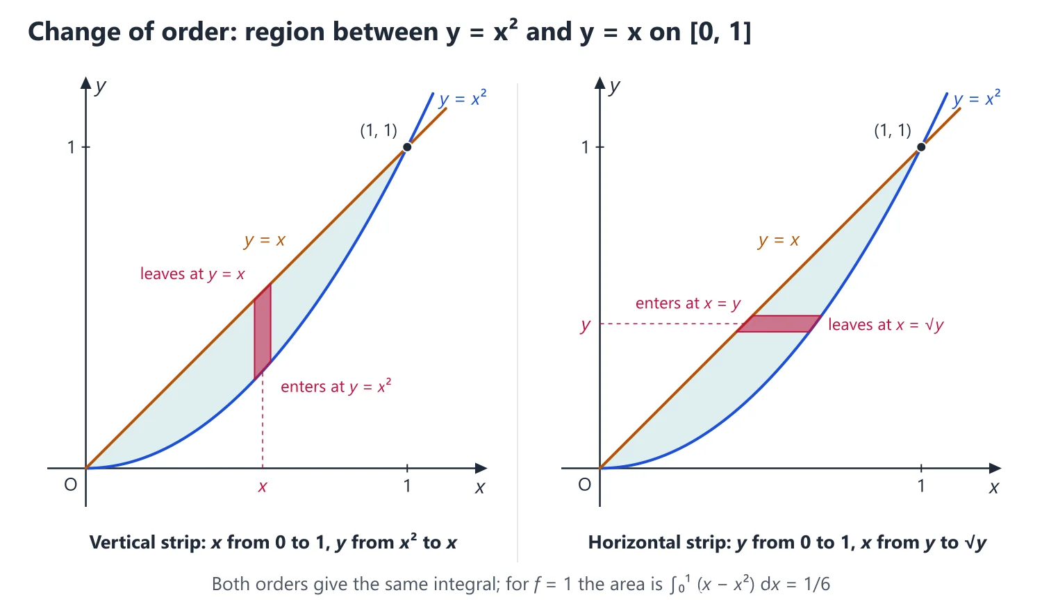
1. Understanding Double Integrals as Repeated Integrals
Why we need it: the volume under a surface, the mass of a plate whose density varies, and the area of a curved region all require adding f(x, y) over a two-dimensional region. Repeated integration reduces this to two single integrals, which we already know how to do.
In words: ∬R f dA is the limit of sums ∑f(xi, yi)ΔAi over small cells covering R, as the cells shrink.
For a region between the curves y = φ1(x) and y = φ2(x), a ≤ x ≤ b: fix x, integrate in y from the lower curve to the upper curve (a vertical strip), then add the strips from x = a to x = b.
The limits of the inner integral may depend on the outer variable; the limits of the outer integral must be constants.
First example, slowly: evaluate ∬R xy dA, where R is the region between y = x2 and y = x.
Step 1: sketch. The curves meet where x2 = x, at (0, 0) and (1, 1); for 0 < x < 1, x2 < x, so the parabola is the lower curve.
Step 2: a vertical strip at x runs from y = x2 up to y = x.
Step 3: inner integral: ∫x2x xy dy = x[y2/2]x2x = (x3 − x5)/2.
Step 4: outer integral: ∫01 (x3 − x5)/2 dx = (1/2)(1/4 − 1/6) = 1/24.
Step 5: check with horizontal strips: for fixed y, x runs from y to √y, ∫y√y xy dx = (y2 − y3)/2, and ∫01 (y2 − y3)/2 dy = (1/2)(1/3 − 1/4) = 1/24 again.
Non-example: the expression ∫01∫x2x f dx dy has no meaning: the inner integration is in x, yet its limits contain x. The condition that fails is that inner limits may depend only on the outer variable.
Building up: (1) for f ≥ 0 the inner integral is the area of the cross-section of the solid at a fixed x, and integrating the cross-sections gives the volume (the slice method).
(2) Fubini's theorem says that for continuous f both orders give the same answer, so choose the order with the easier limits or the easier inner integral.
(3) To change the order, rewrite the region as inequalities in the other order, read from the sketch, and split the region wherever a strip would end on a different curve.
(4) With f = 1 the double integral is the area of R, which is how areas are found below.
Where it is used: change-of-order questions, areas between curves, and centres of mass and moments of inertia in Mechanics.
2. Understanding Change of Variables and Polar Coordinates
Why we need it: discs, sectors and ellipses give awkward Cartesian limits such as √(a2 − x2), and integrands with x2 + y2 are hard to integrate. In suitable new variables the region becomes a rectangle and the integrand simplifies.
But small areas change size under the change, so a correction factor is needed.
In words: let x = x(u, v), y = y(u, v) map a region S of the uv-plane one-to-one onto R. Then ∬R f dx dy = ∬S f(x(u, v), y(u, v))|J| du dv, where J = ∂(x, y)/∂(u, v).
|J| is the factor by which a tiny rectangle du × dv is stretched. In polar coordinates J = r, so dx dy = r dr dθ: a polar cell has sides dr and r dθ.
First example, slowly: evaluate ∬(x2 + y2) dx dy over the disc x2 + y2 ≤ 4.
Step 1: in polar coordinates the disc is 0 ≤ r ≤ 2, 0 ≤ θ ≤ 2π, a rectangle in the (r, θ)-plane.
Step 2: the integrand x2 + y2 becomes r2.
Step 3: the element dx dy becomes r dr dθ.
Step 4: ∫02π∫02 r2·r dr dθ = 2π[r4/4]02 = 2π·4 = 8π.
Step 5: notice the extra factor r; forgetting it gives 2π·8/3 = 16π/3, which is wrong.
Non-example: u = x2, v = y on the rectangle −1 ≤ x ≤ 1, 0 ≤ y ≤ 1 is not one-to-one: x and −x give the same u, and the Jacobian 2x vanishes on x = 0.
Applying the formula once over 0 ≤ u ≤ 1 counts only half of the rectangle. The condition that fails is one-to-one; the remedy is to split the rectangle into x ≥ 0 and x ≤ 0 and use the formula on each half.
Building up: (1) a tiny rectangle with sides du, dv is carried to an almost-parallelogram spanned by (xu, yu)du and (xv, yv)dv, because the map is differentiable.
(2) Its area is |xuyv − xvyu| du dv = |J| du dv (derivation below).
(3) Adding these pieces gives the formula. When the new variables are given as u(x, y), v(x, y), use |J| = 1/|∂(u, v)/∂(x, y)| instead of inverting the map.
(4) Standard factors: polar r, elliptic polar abr, linear |ad − bc| (see the tables of this topic and the previous one).
Where it is used: the Gaussian integral, areas inside cardioids and circles, and regions bounded by curves such as xy = c or x2 − y2 = c (see the Solved UPSC Questions below).
3. Double Integrals
Over a region R, ∬R f(x, y) dx dy. If R = {a ≤ x ≤ b, φ1(x) ≤ y ≤ φ2(x)}, the integral is ∫ab [∫φ1(x)φ2(x) f dy] dx; the inner integral, with variable limits, is evaluated first.
Idea: for f ≥ 0, ∬R f dx dy is the volume of the solid between the surface z = f(x, y) and the region R. The inner integral ∫f dy is the area of the cross-section at a fixed x, and integrating these cross-sections over x gives the volume (the slice method).
Fubini's theorem: for f continuous on a rectangle (or a region of the above type), the double integral equals either repeated integral, so the order of integration may be interchanged.
Continuity (or at least boundedness) matters: for f = (x2 − y2)/(x2 + y2)2 on 0 < x, y ≤ 1, integrating first in y gives ∫01 dx/(1 + x2) = π/4, while integrating first in x gives −π/4, because f is unbounded near the origin.
Change of order (method): (1) write the limits as inequalities; (2) sketch the region; (3) draw strips in the other direction and read off the new limits, splitting the region wherever a strip would end on different boundary curves.
See the figure above: for the region between y = x2 and y = x on [0, 1], vertical strips run from y = x2 up to y = x and horizontal strips from x = y to x = √y, so ∫01∫x2x f dy dx = ∫01∫y√y f dx dy.
Change of variables: ∬ f(x, y) dx dy = ∬ f(x(u, v), y(u, v)) |∂(x, y)/∂(u, v)| du dv; in polar coordinates dx dy = r dr dθ.
Derivation: a small rectangle du × dv in the uv-plane is carried to an approximate parallelogram spanned by (xu, yu)du and (xv, yv)dv, whose area is |xuyv − xvyu| du dv = |∂(x, y)/∂(u, v)| du dv. In polar coordinates the element is a curvilinear rectangle with sides dr and r dθ, so dx dy = r dr dθ.
Bounds for an integral: if m ≤ f ≤ M on R, then m·(area of R) ≤ ∬R f dx dy ≤ M·(area of R).
Splitting the region: for an integrand containing |g(x, y)| or defined piecewise, split R along the curve g = 0 (or along the curves bounding the pieces) and integrate over each part.
Change of variables given as u(x, y), v(x, y): use dx dy = du dv/|∂(u, v)/∂(x, y)|, which avoids inverting the map; check that the map is one-one on the region and find the new limits from the boundary curves.
4. Understanding Triple Integrals and Spherical Coordinates
Why we need it: volumes, masses and moments of inertia of solids require adding over three-dimensional regions. As with double integrals, we reduce the job to repeated single integrals.
In words: in ∭V f dV with Cartesian coordinates, for fixed (x, y) let z run from the lower surface to the upper surface, then integrate over the projection D of the solid on the xy-plane. The innermost limits are surfaces, the middle limits curves, and the outer limits numbers.
Cylindrical coordinates (r, θ, z) have dV = r dr dθ dz. In spherical coordinates (r, θ, φ), r is the distance from the origin, θ the angle from the positive z-axis (0 to π) and φ the angle around the z-axis (0 to 2π), and dV = r2 sin θ dr dθ dφ.
First example, slowly: find the volume of the solid between the cone z = √(x2 + y2) and the plane z = 1.
Step 1: the cone meets the plane on the circle x2 + y2 = 1, so for (x, y) in the unit disc, z runs from √(x2 + y2) up to 1.
Step 2: in cylindrical coordinates √(x2 + y2) = r, so the solid is r ≤ z ≤ 1, 0 ≤ r ≤ 1, 0 ≤ θ ≤ 2π.
Step 3: V = ∫02π∫01∫r1 r dz dr dθ.
Step 4: the innermost integral is ∫r1 r dz = r(1 − r).
Step 5: the middle integral is ∫01 (r − r2) dr = 1/2 − 1/3 = 1/6.
Step 6: the outer integral gives V = 2π/6 = π/3, which agrees with (1/3)(base area)(height) = (1/3)π(1)(1) for a cone.
Non-example: writing the spherical element as r2 dr dθ dφ, without sin θ, gives the ball of radius a the 'volume' ∫02π∫0π∫0a r2 dr dθ dφ = 2π2a3/3 instead of 4πa3/3.
The missing factor sin θ records that circles of latitude near the poles are short: the circle at angle θ has radius r sin θ.
Building up: (1) the innermost integral over z turns the triple integral into a double integral; with f = 1 it is the height h − g, so V = ∬D (h − g) dx dy.
(2) The spherical box has edges dr, r dθ and r sin θ dφ, so dV = r2 sin θ dr dθ dφ (derivation below), which equals the Jacobian ∂(x, y, z)/∂(r, θ, φ).
(3) Over x + y + z ≤ 1 with a power integrand, repeated Beta integrals give Dirichlet's formula, so no limits need to be written at all.
Where it is used: volumes between paraboloids, sphere–cylinder intersections, ∭xyz over an octant, centres of gravity and moments of inertia in Mechanics, and the divergence theorem in Vector Analysis.
5. Triple Integrals
∭V f dx dy dz is evaluated as three successive single integrals; use cylindrical coordinates (dV = r dr dθ dz) or spherical coordinates (dV = r2 sin θ dr dθ dφ) when the region has that symmetry.
Derivation of the spherical element: with x = r sin θ cos φ, y = r sin θ sin φ, z = r cos θ (θ measured from the z-axis), the element is a curved box with edges dr, r dθ (along a meridian) and r sin θ dφ (along a circle of latitude of radius r sin θ), so dV = r2 sin θ dr dθ dφ, which agrees with ∂(x, y, z)/∂(r, θ, φ) = r2 sin θ.
Dirichlet's integral: ∭ xl−1ym−1zn−1 dx dy dz over x, y, z ≥ 0, x + y + z ≤ 1 equals Γ(l)Γ(m)Γ(n)/Γ(l + m + n + 1).
Derivation (two variables): over x, y ≥ 0, x + y ≤ 1, the inner integral is ∫01−x ym−1 dy = (1 − x)m/m, and then ∫01 xl−1(1 − x)m dx/m = β(l, m + 1)/m = Γ(l)Γ(m + 1)/(mΓ(l + m + 1)) = Γ(l)Γ(m)/Γ(l + m + 1). One more integration in the same way gives the three-variable formula; for x/a + y/b + z/c ≤ 1 first put x = au, y = bv, z = cw.
Liouville's extension: over x, y, z ≥ 0 with x + y + z ≤ h, ∭ f(x + y + z)xl−1ym−1zn−1 dx dy dz = (Γ(l)Γ(m)Γ(n)/Γ(l + m + n)) ∫0h f(u)ul+m+n−1 du.
Volume between two surfaces: if g(x, y) ≤ z ≤ h(x, y) over D, then V = ∭ dz dy dx = ∬D (h − g) dx dy, where D is found by projecting the curve h = g onto the xy-plane. The tetrahedron x/a + y/b + z/c ≤ 1 in the first octant has V = abc/6.
6. Areas
Cartesian: A = ∬R dx dy = ∫ab (y2 − y1) dx. Polar: A = (1/2)∫αβ r2 dθ = ∬ r dr dθ. Closed curve given parametrically: A = (1/2)∮(x dy − y dx).
Derivation: a thin sector between θ and θ + dθ is nearly a circular sector of radius r, with area (1/2)r2 dθ; adding these sectors gives (1/2)∫r2 dθ. The formula (1/2)∮(x dy − y dx) is Green's theorem with P = −y/2, Q = x/2, since ∂Q/∂x − ∂P/∂y = 1.
Area between polar curves r1(θ) ≤ r ≤ r2(θ), α ≤ θ ≤ β: A = (1/2)∫αβ (r22 − r12) dθ, with the limits of θ found from r1 = r2.
Area common to two curves: find the points of intersection, use symmetry, and choose strips (vertical or horizontal) so that each strip runs between the same two curves.
7. Understanding Volumes and Surfaces of Revolution
Why we need it: many solids, such as the sphere, the cone, the torus and paraboloid bowls, are made by spinning a plane region about an axis. Slicing across the axis gives discs and spinning an arc gives thin bands, so these problems reduce to single integrals.
In words: for the volume, the slice at x is a disc of radius y = f(x) and thickness dx, so dV = πy2 dx.
For the surface, a short arc ds at height y sweeps a band of circumference 2πy and width ds, so dS = 2πy ds, where ds = √(1 + (dy/dx)2) dx accounts for the slope of the arc.
Pappus' theorems say the same in one line: volume = area × distance travelled by the centroid of the area; surface = arc length × distance travelled by the centroid of the arc.
First example, slowly: revolve y = √(a2 − x2), −a ≤ x ≤ a, about the x-axis to get a sphere of radius a.
Step 1: volume: V = π∫−aa (a2 − x2) dx = π(2a3 − 2a3/3) = 4πa3/3.
Step 2: for the surface, dy/dx = −x/√(a2 − x2), so 1 + (dy/dx)2 = a2/(a2 − x2) and √(1 + (dy/dx)2) = a/y.
Step 3: dS = 2πy·(a/y) dx = 2πa dx; the y cancels.
Step 4: S = 2πa·2a = 4πa2.
Step 5: notice that the band area per unit length of x is constant, so any slab of thickness h cut from the sphere by two parallel planes has curved surface 2πah (Archimedes).
Non-example: using 2π∫y dx for the sphere gives 2π(πa2/2) = π2a2 ≈ 9.87a2, not 4πa2 ≈ 12.57a2. The step that fails is the width of the band: it is ds, not dx, and on a sloping arc ds > dx.
Building up: (1) Pythagoras gives ds2 = dx2 + dy2, which yields all the forms of arc length (derivation below).
(2) The disc and band elements give V = π∫y2 dx and S = 2π∫y ds.
(3) Pappus follows from the definition of the centroid: an element dA at distance y from the axis sweeps the volume 2πy dA, and ∫2πy dA = 2πȳA, where ȳ is the distance of the centroid from the axis.
(4) In polar form, the element of area (1/2)r2 dθ has its centroid at height (2/3)r sin θ, so Pappus gives V = (2π/3)∫r3 sin θ dθ.
Where it is used: volumes and surfaces generated by the cardioid, the astroid and loops of curves, the torus, and the centroids needed in Statics.
8. Arc Length, Surface Area and Volume
Arc length: s = ∫ √(1 + (dy/dx)2) dx = ∫ √(r2 + (dr/dθ)2) dθ = ∫ √((dx/dt)2 + (dy/dt)2) dt.
Derivation: for a short piece of the curve ds2 = dx2 + dy2 (Pythagoras), which gives all three forms; in polar coordinates dx2 + dy2 = dr2 + r2dθ2.
Volume of revolution about the x-axis: V = π∫ab y2 dx. A polar region bounded by r = f(θ), α ≤ θ ≤ β, revolved about the initial line: V = (2π/3)∫αβ r3 sin θ dθ.
Derivation: a thin slice at x is a disc of radius y and thickness dx, with volume πy2 dx. For the polar form, the triangular element of area (1/2)r2 dθ has its centroid at distance (2/3)r sin θ from the initial line, so Pappus' theorem gives dV = 2π·(2/3)r sin θ·(1/2)r2 dθ = (2π/3)r3 sin θ dθ.
Surface of revolution about the x-axis: S = 2π∫ y ds = 2π∫ab y√(1 + (dy/dx)2) dx.
Derivation: a short arc ds at height y sweeps out a thin band (a frustum of a cone) of radius y and slant height ds, with area 2πy ds. Writing 2π∫y dx instead is wrong, because it ignores the slope of the arc.
Pappus' theorems: volume = (area of the region) × (distance travelled by its centroid); surface area = (length of the arc) × (distance travelled by the centroid of the arc); the axis must not cut the region.
For instance, the torus obtained by revolving a circle of radius a about a line at distance b > a from its centre has V = πa2·2πb = 2π2a2b and S = 2πa·2πb = 4π2ab.
Volume under a surface: V = ∬R z dx dy, or V = ∭ dx dy dz. Surface area of z = f(x, y) over R: S = ∬R √(1 + zx2 + zy2) dx dy.
Derivation of the surface formula: the piece of the tangent plane above a small rectangle dx dy has area dx dy/|cos γ|, where γ is the angle between the normal (−zx, −zy, 1) and the z-axis; since |cos γ| = 1/√(1 + zx2 + zy2), the element of surface is √(1 + zx2 + zy2) dx dy.
9. Choosing the Method
If the inner integral cannot be done in elementary terms (ex2, (sin y)/y, e−y2) → change the order of integration; the new inner integral usually becomes elementary.
If the region or the integrand has circular, cylindrical or spherical symmetry → change coordinates as in the second table of this topic; if the region is x + y + z ≤ h with a power integrand → Dirichlet's or Liouville's integral.
If a volume or surface of revolution of a region with a known centroid is asked → Pappus' theorems give it in one line.
10. Common Mistakes
Forgetting the factor r in polar coordinates or r2 sin θ in spherical coordinates.
Changing the order of integration by merely interchanging the limits, without redrawing the region; the new limits must be read from the sketch, and the region may need splitting.
Multiplying by 4 for symmetry when the integrand is not even in both x and y.
Using 2π∫y dx for a surface of revolution instead of 2π∫y ds.
Applying Pappus when the axis cuts the region, or using the centroid of the area in a surface problem, where the centroid of the arc is needed.
Leaving the answer as an unevaluated Gamma expression when it simplifies (Γ(1/2) = √π, Γ(n + 1) = n!).
11. Connections
Link: Green's theorem in the plane, Stokes' theorem and Gauss's divergence theorem convert line, surface and volume integrals into one another, and the area formula (1/2)∮(x dy − y dx) is the simplest case (Vector Analysis).
Link: centres of mass and moments of inertia in Mechanics are multiple integrals of exactly this kind.
Link: Dirichlet's integral reduces to Beta and Gamma functions (previous topic), and the Jacobian of every substitution is the determinant studied in Functions of Several Variables.
12. Worked Examples
Example 1: Change the order of integration and evaluate ∫0∞∫x∞ (e−y/y) dy dx.
The region is 0 ≤ x ≤ y < ∞. With the order reversed, x runs from 0 to y: ∫0∞ (e−y/y)·y dy = ∫0∞ e−y dy = 1.
Example 2: Evaluate ∬ e−(x2+y2) dx dy over the first quadrant and deduce ∫0∞ e−x2 dx.
In polar coordinates the integral is ∫0π/2∫0∞ e−r2 r dr dθ = (π/2)(1/2) = π/4. It also equals I2, where I = ∫0∞ e−x2 dx, so I = √π/2.
Example 3: Find the volume of the sphere x2 + y2 + z2 = a2 by a triple integral.
V = ∫02π∫0π∫0a r2 sin θ dr dθ dφ = (a3/3)(2)(2π) = 4πa3/3.
Example 4: Find the area of the part of the sphere x2 + y2 + z2 = a2 lying inside the cylinder x2 + y2 = ax (Viviani's problem).
For the upper half, √(1 + zx2 + zy2) = a/√(a2 − r2), so S = ∫−π/2π/2∫0a cos θ ar dr dθ/√(a2 − r2) = ∫−π/2π/2 a2(1 − |sin θ|) dθ = a2(π − 2). Both halves together give 2a2(π − 2).
Example 5: The volume generated by revolving the cardioid r = a(1 + cos θ) about the initial line is V = (2π/3)∫0π a3(1 + cos θ)3 sin θ dθ = (2π/3)a3·4 = 8πa3/3.
Example 6: Evaluate ∬R (x + y)2 dx dy, where R is the parallelogram bounded by x + y = 0, x + y = 2, 3x − 2y = 0 and 3x − 2y = 3.
Put u = x + y, v = 3x − 2y; R becomes the rectangle 0 ≤ u ≤ 2, 0 ≤ v ≤ 3.
∂(u, v)/∂(x, y) = det [[1, 1], [3, −2]] = −5, so dx dy = |∂(x, y)/∂(u, v)| du dv = (1/5) du dv.
Integral = (1/5)∫03∫02 u2 du dv = (1/5)(8/3)(3) = 8/5.
Example 7: Evaluate ∭ xyz dx dy dz over the positive octant of the sphere x2 + y2 + z2 ≤ a2.
In spherical coordinates xyz = r3 sin2θ cos θ sin φ cos φ and dV = r2 sin θ dr dθ dφ, with 0 ≤ r ≤ a, 0 ≤ θ ≤ π/2, 0 ≤ φ ≤ π/2.
The integral separates: ∫0a r5 dr · ∫0π/2 sin3θ cos θ dθ · ∫0π/2 sin φ cos φ dφ = (a6/6)(1/4)(1/2) = a6/48.
13. Solved UPSC Questions
Example 8 (UPSC 2014, 15 marks): By using the transformation x + y = u, y = uv, evaluate the integral ∬ {xy(1 − x − y)}1/2 dx dy taken over the area enclosed by the straight lines x = 0, y = 0 and x + y = 1.
x + y = u, y = uv give x = u(1 − v), y = uv; the triangle x ≥ 0, y ≥ 0, x + y ≤ 1 becomes the square 0 ≤ u ≤ 1, 0 ≤ v ≤ 1.
∂(x, y)/∂(u, v) = det [[1 − v, −u], [v, u]] = u(1 − v) + uv = u, so dx dy = u du dv.
xy(1 − x − y) = u2v(1 − v)(1 − u), so the integral is ∫01∫01 u2(1 − u)1/2v1/2(1 − v)1/2 du dv = β(3, 3/2)β(3/2, 3/2).
β(3, 3/2) = Γ(3)Γ(3/2)/Γ(9/2) = 2(√π/2)/((105/16)√π) = 16/105 and β(3/2, 3/2) = (√π/2)2/Γ(3) = π/8.
Answer: (16/105)(π/8) = 2π/105.
Example 9 (UPSC 2015, 13 marks): Evaluate ∬R √|y − x2| dx dy where R = [−1, 1 ; 0, 2].
Split R = [−1, 1] × [0, 2] along y = x2: R1: x2 ≤ y ≤ 2 and R2: 0 ≤ y ≤ x2 (−1 ≤ x ≤ 1).
On R2: ∫0x2 √(x2 − y) dy = (2/3)|x|3, and ∫−11 (2/3)|x|3 dx = 1/3.
On R1: ∫x22 √(y − x2) dy = (2/3)(2 − x2)3/2, and ∫−11 (2/3)(2 − x2)3/2 dx = (4/3)∫01 (2 − x2)3/2 dx.
With x = √2 sin θ (0 ≤ θ ≤ π/4): ∫01 (2 − x2)3/2 dx = ∫0π/4 4 cos4θ dθ = (1/2)∫0π/4 (3 + 4 cos 2θ + cos 4θ) dθ = (1/2)(3π/4 + 2) = 3π/8 + 1.
So the R1 part is (4/3)(3π/8 + 1) = π/2 + 4/3, and the total is π/2 + 4/3 + 1/3.
Answer: π/2 + 5/3 ≈ 3.237.
Example 10 (UPSC 2016, 15 marks): Find the surface area of the plane x + 2y + 2z = 12 cut off by x = 0, y = 0 and x2 + y2 = 16.
On the plane z = (12 − x − 2y)/2, so zx = −1/2, zy = −1 and √(1 + zx2 + zy2) = √(1 + 1/4 + 1) = 3/2.
The portion cut off by x = 0, y = 0 and the cylinder x2 + y2 = 16 projects onto the quarter disc D: x, y ≥ 0, x2 + y2 ≤ 16, of area 4π (z stays positive there).
S = ∬D (3/2) dx dy = (3/2)(4π). (Equivalently, S = (area of projection)/cos γ with cos γ = 2/3 for the unit normal (1, 2, 2)/3.)
Answer: 6π.
Example 11 (UPSC 2016, 15 marks): Evaluate ∬R f(x, y) dx dy over the rectangle R = [0, 1; 0, 1] where
f(x, y) = x + y, if x2 < y < 2x2
f(x, y) = 0, elsewhere
f is non-zero only between the parabolas y = x2 and y = 2x2 inside the square, and 2x2 ≤ 1 for x ≤ 1/√2. f is bounded with discontinuities only on two curves, so it is integrable.
For 0 ≤ x ≤ 1/√2, y runs from x2 to 2x2: ∫(x + y) dy = x3 + 3x4/2, and ∫01/√2 (x3 + 3x4/2) dx = 1/16 + 3/(40√2).
For 1/√2 ≤ x ≤ 1, y runs from x2 to 1: ∫(x + y) dy = x − x3 + (1 − x4)/2, and ∫1/√21 = [x2/2 − x4/4 + x/2 − x5/10]1/√21 = 13/20 − 3/16 − 19/(40√2).
Total = 1/16 + 13/20 − 3/16 − 16/(40√2) = 21/40 − √2/5.
Answer: 21/40 − √2/5 ≈ 0.242.
Example 12 (UPSC 2017, 10 marks): Integrate the function f(x, y) = xy(x2 + y2) over the domain R : {−3 ≤ x2 − y2 ≤ 3, 1 ≤ xy ≤ 4}.
Put u = x2 − y2, v = xy. Then ∂(u, v)/∂(x, y) = det [[2x, −2y], [y, x]] = 2(x2 + y2), so dx dy = du dv/(2(x2 + y2)).
Hence xy(x2 + y2) dx dy = (v/2) du dv.
In the first quadrant the map is one-one onto the rectangle −3 ≤ u ≤ 3, 1 ≤ v ≤ 4 (it is z ↦ z2 with z = x + iy, since z2 = u + 2iv), so the integral is (1/2)∫−33 du ∫14 v dv = (1/2)(6)(15/2) = 45/2.
[The set 1 ≤ xy ≤ 4 also has a branch in the third quadrant, where the integrand takes the same values; the intended region is the first-quadrant one. If both branches are counted, the integral is 45.]
Answer: 45/2 (over the first-quadrant region).
Example 13 (UPSC 2017, 15 marks): Find the volume of the solid above the xy-plane and directly below the portion of the elliptic paraboloid x2 + y2/4 = z which is cut off by the plane z = 9.
The paraboloid z = x2 + y2/4 meets z = 9 above the ellipse E: x2 + y2/4 ≤ 9 (semi-axes 3 and 6, area 18π). The solid above z = 0 and below this portion has V = ∬E (x2 + y2/4) dx dy.
Put x = r cos θ, y = 2r sin θ (Jacobian 2r): E becomes 0 ≤ r ≤ 3, 0 ≤ θ ≤ 2π, and the integrand is r2.
V = ∫02π∫03 r2·2r dr dθ = 2π · 2 · 81/4 = 81π. (The solid inside the paraboloid up to z = 9 has volume 9 · 18π − 81π = 81π as well, so both readings agree.)
Answer: 81π.
Example 14 (UPSC 2017, 10 marks): Prove that π/3 ≤ ∬D dx dy/√(x2 + (y − 2)2) ≤ π where D is the unit disc.
f(x, y) = 1/√(x2 + (y − 2)2) = 1/d, where d is the distance from (x, y) to P(0, 2), and |OP| = 2.
For (x, y) in the unit disc D, the triangle inequality gives 2 − 1 ≤ d ≤ 2 + 1, i.e. 1 ≤ d ≤ 3 (attained at (0, 1) and (0, −1)); hence 1/3 ≤ f ≤ 1 on D.
With m = 1/3, M = 1 and area(D) = π: m·π ≤ ∬D f dx dy ≤ M·π.
Answer: π/3 ≤ ∬D dx dy/√(x2 + (y − 2)2) ≤ π.
Example 15 (UPSC 2018, 12 marks): Evaluate the integral ∫0a ∫x/ax x dy dx/(x2 + y2).
Inner integral (x > 0 fixed): ∫x/ax x dy/(x2 + y2) = [tan−1(y/x)]y=x/ay=x = π/4 − tan−1(1/a), which does not depend on x.
Outer integral: ∫0a (π/4 − tan−1(1/a)) dx = a(π/4 − tan−1(1/a)).
Since tan(π/4 − φ) = (1 − tan φ)/(1 + tan φ), this also equals a tan−1((a − 1)/(a + 1)) for a > 0.
Answer: a(π/4 − tan−1(1/a)) = a tan−1((a − 1)/(a + 1)).
Example 16 (UPSC 2021, 15 marks): Show that the entire area of the Astroid : x2/3 + y2/3 = a2/3 is (3/8)πa2.
Parametrise the astroid by x = a cos3t, y = a sin3t. It is symmetric about both axes, so A = 4∫0a y dx (first quadrant).
As x goes from 0 to a, t goes from π/2 to 0, and dx = −3a cos2t sin t dt; so A = 4∫π/20 a sin3t(−3a cos2t sin t) dt = 12a2∫0π/2 sin4t cos2t dt.
By Wallis' formula ∫0π/2 sin4t cos2t dt = (3·1·1)/(6·4·2)·(π/2) = π/32.
Answer: A = 12a2(π/32) = (3/8)πa2.
Example 17 (UPSC 2022, 15 marks): Use double integration to calculate the area common to the circle x2 + y2 = 4 and the parabola y2 = 3x.
Intersection: x2 + 3x = 4 gives x = 1 (x = −4 is impossible since 3x = y2 ≥ 0), so the points are (1, ±√3). The common region is symmetric about the x-axis.
Horizontal strips: for −√3 ≤ y ≤ √3, x runs from the parabola x = y2/3 to the circle x = √(4 − y2). A = ∫−√3√3∫y2/3√(4−y2) dx dy = 2∫0√3 (√(4 − y2) − y2/3) dy.
∫0√3 √(4 − y2) dy = [y√(4 − y2)/2 + 2 sin−1(y/2)]0√3 = √3/2 + 2π/3, and ∫0√3 (y2/3) dy = √3/3.
A = 2(√3/2 + 2π/3 − √3/3) = 4π/3 + √3/3.
Answer: (4π + √3)/3 square units.
Example 18 (UPSC 2023, 15 marks): Evaluate the triple integral which gives the volume of the solid enclosed between the two paraboloids Z = 5(x2 + y2) and Z = 6 − 7x2 − y2.
The surfaces meet where 5(x2 + y2) = 6 − 7x2 − y2, i.e. 2x2 + y2 = 1. The solid lies over the ellipse E: 2x2 + y2 ≤ 1, between z = 5(x2 + y2) below and z = 6 − 7x2 − y2 above.
V = ∬E ∫5(x2+y2)6−7x2−y2 dz dx dy = ∬E (6 − 12x2 − 6y2) dx dy = 6∬E (1 − 2x2 − y2) dx dy.
Put x = r cos θ/√2, y = r sin θ (Jacobian r/√2): V = 6∫02π∫01 (1 − r2)(r/√2) dr dθ = (6/√2)(2π)(1/4).
Answer: V = 3π/√2 = (3√2/2)π ≈ 6.66 cubic units.
Example 19 (UPSC 2024, 15 marks): Using double integration, find the area lying inside the cardioid r = a(1 + cos θ) and outside the circle r = a.
The curves meet where a(1 + cos θ) = a, i.e. θ = ±π/2, and the cardioid lies outside the circle for −π/2 ≤ θ ≤ π/2 (where cos θ ≥ 0).
A = ∫−π/2π/2∫aa(1+cos θ) r dr dθ = (a2/2)∫−π/2π/2 [(1 + cos θ)2 − 1] dθ = (a2/2)∫−π/2π/2 (2 cos θ + cos2θ) dθ.
∫−π/2π/2 2 cos θ dθ = 4 and ∫−π/2π/2 cos2θ dθ = π/2, so A = (a2/2)(4 + π/2).
Answer: A = a2(8 + π)/4.
Example 20 (UPSC 2025, 20 marks): (i) Evaluate ∬R y dx dy, where R is the region bounded by y = x and y = 4x − x2. (10 marks)
(ii) If u(x, y) = x f(y/x) + g(y/x), where f and g are arbitrary functions, then show that
I. x ∂u/∂x + y ∂u/∂y = x f(y/x),
II. x2 ∂2u/∂x2 + 2xy ∂2u/∂x∂y + y2 ∂2u/∂y2 = 0. (10 marks)
(i) The curves meet where x = 4x − x2, i.e. x = 0 and x = 3, and 4x − x2 ≥ x on [0, 3]. So ∬R y dx dy = ∫03∫x4x−x2 y dy dx = (1/2)∫03 [(4x − x2)2 − x2] dx.
= (1/2)∫03 (15x2 − 8x3 + x4) dx = (1/2)(135 − 162 + 243/5) = (1/2)(108/5) = 54/5.
(ii) Assume f, g have continuous second derivatives. v = x f(y/x) is homogeneous of degree 1 and w = g(y/x) of degree 0 (replacing x, y by tx, ty multiplies them by t and by 1).
I. By Euler's theorem xvx + yvy = v and xwx + ywy = 0; adding, xux + yuy = v = x f(y/x).
II. The second-order form gives x2vxx + 2xyvxy + y2vyy = 1(1 − 1)v = 0, and the same expression in w equals 0(0 − 1)w = 0; adding gives the result.
Answer: (i) 54/5; (ii) both identities hold.
Example 21 (UPSC 2026, 20 marks): (i) Evaluate the double integral ∫02 ∫x2+12x+1 x2y dy dx by reversing the order of integration. (10)
(ii) Find the volume of the solid, which is formed from the intersection of the coordinate planes x = 0, y = 0, z = 0 and the plane x/a + y/b + z/c = 1. (10)
(i) Region: 0 ≤ x ≤ 2, x2 + 1 ≤ y ≤ 2x + 1; the parabola and the line meet at (0, 1) and (2, 5). For 1 ≤ y ≤ 5, x runs from the line, x = (y − 1)/2, to the parabola, x = √(y − 1).
I = ∫15∫(y−1)/2√(y−1) x2y dx dy = ∫15 (y/3)[(y − 1)3/2 − (y − 1)3/8] dy.
With t = y − 1: I = (1/3)∫04 (t + 1)(t3/2 − t3/8) dt = (1/3)[2t7/2/7 + 2t5/2/5 − t5/40 − t4/32]04 = (1/3)(256/7 + 64/5 − 128/5 − 8) = (1/3)(552/35) = 184/35.
Check in the original order: (1/2)∫02 x2[(2x + 1)2 − (x2 + 1)2] dx = (1/2)∫02 (4x3 + 2x4 − x6) dx = (1/2)(16 + 64/5 − 128/7) = 184/35.
(ii) The tetrahedron is 0 ≤ x ≤ a, 0 ≤ y ≤ b(1 − x/a), 0 ≤ z ≤ c(1 − x/a − y/b) (a, b, c > 0). V = ∫0a∫0b(1−x/a) c(1 − x/a − y/b) dy dx = ∫0a (bc/2)(1 − x/a)2 dx = abc/6.
Answer: (i) 184/35; (ii) abc/6.
14. Practice Exercises
Exercise 1 (basic): Evaluate ∫01∫02 (x + y) dy dx.
Answer: the inner integral is 2x + 2, and ∫01 (2x + 2) dx = 3.
Exercise 2 (basic): Using a double integral, find the area between y = x2 and y = 2x.
Answer: the curves meet at x = 0 and x = 2; A = ∫02∫x22x dy dx = 4 − 8/3 = 4/3.
Exercise 3 (basic): Change the order of integration in ∫01∫0x f(x, y) dy dx.
Answer: the region is the triangle 0 ≤ y ≤ x ≤ 1, so the integral is ∫01∫y1 f(x, y) dx dy.
Exercise 4 (standard): Evaluate ∫01∫x1 sin(y2) dy dx by changing the order of integration.
Answer: ∫01∫0y sin(y2) dx dy = ∫01 y sin(y2) dy = (1 − cos 1)/2.
Exercise 5 (standard): Evaluate ∬ dx dy/(x2 + y2) over the annulus 1 ≤ x2 + y2 ≤ 4.
Answer: in polar coordinates ∫02π∫12 (1/r2) r dr dθ = 2π log 2.
Exercise 6 (standard): Find the volume of the solid bounded by the paraboloid z = 4 − x2 − y2 and the plane z = 0.
Answer: V = ∫02π∫02 (4 − r2) r dr dθ = 2π(8 − 4) = 8π.
Exercise 7 (standard): Find the total length of the cardioid r = a(1 + cos θ).
Answer: r2 + (dr/dθ)2 = 2a2(1 + cos θ) = 4a2cos2(θ/2), so s = 2∫0π 2a cos(θ/2) dθ = 8a.
Exercise 8 (UPSC level): Evaluate ∭(x2 + y2 + z2) dx dy dz over the ball x2 + y2 + z2 ≤ a2.
Answer: in spherical coordinates ∫02π∫0π∫0a r4 sin θ dr dθ dφ = (a5/5)(2)(2π) = 4πa5/5.
Exercise 9 (UPSC level): Find the area of the part of the paraboloid z = x2 + y2 that lies below the plane z = 1.
Answer: √(1 + zx2 + zy2) = √(1 + 4r2), so S = ∫02π∫01 √(1 + 4r2) r dr dθ = (π/6)(5√5 − 1).
Exercise 10 (UPSC level): Find the volume of the part of the ball x2 + y2 + z2 ≤ a2 that lies inside the cylinder x2 + y2 = ax.
Answer: V = 2∫−π/2π/2∫0a cos θ √(a2 − r2) r dr dθ = (2a3/3)∫−π/2π/2 (1 − |sin θ|3) dθ = (2a3/3)(π − 4/3).
| Quantity | Cartesian y = f(x) | Polar r = f(θ) | Parametric x(t), y(t) |
|---|---|---|---|
| Area | ∫ y dx | (1/2)∫ r2 dθ | ∫ y (dx/dt) dt or (1/2)∮(x dy − y dx) |
| Arc length | ∫ √(1 + (dy/dx)2) dx | ∫ √(r2 + (dr/dθ)2) dθ | ∫ √((dx/dt)2 + (dy/dt)2) dt |
| Volume about x-axis (initial line) | π∫ y2 dx | (2π/3)∫ r3 sin θ dθ | π∫ y2 (dx/dt) dt |
| Surface about x-axis (initial line) | 2π∫ y ds | 2π∫ r sin θ ds | 2π∫ y √((dx/dt)2 + (dy/dt)2) dt |
| Region or integrand | Coordinates | Element | Watch out for |
|---|---|---|---|
| Bounded by straight lines or curves y = g(x) | Cartesian | dx dy | Split the region where a strip changes its boundary curve |
| Circles, sectors, x2 + y2 in the integrand | Polar | r dr dθ | x2 + y2 = 2ax is r = 2a cos θ, −π/2 ≤ θ ≤ π/2 |
| Ellipse x2/a2 + y2/b2 ≤ 1 | x = ar cos θ, y = br sin θ | abr dr dθ | The Jacobian is abr, not r |
| Cylinders, solids symmetric about the z-axis | Cylindrical | r dr dθ dz | Integrate in z first, then over the projection |
| Spheres, cones with vertex at the origin | Spherical | r2 sin θ dr dθ dφ | θ from the z-axis (0 to π), φ around it (0 to 2π) |
| x + y + z ≤ h, integrand a product of powers | Dirichlet or Liouville | Gamma functions | The variables must be non-negative |
| Integrand in x + y and x − y (or xy, y/x) | u, v equal to those expressions | du dv/|∂(u, v)/∂(x, y)| | Find the new limits from each boundary curve |
Mains points
- Change of order of integration is asked very often: draw the region, mark the curves and their points of intersection, and write the new limits; the sketch carries marks.
- Use polar, cylindrical or spherical coordinates whenever the region or integrand contains x2 + y2 or x2 + y2 + z2, and always include the Jacobian factor.
- Volume questions bounded by two surfaces (for example a paraboloid and a plane, or a sphere and a cylinder) are standard 15-mark questions; find the projection of the solid on a coordinate plane first.
- Dirichlet's and Liouville's integrals give quick answers for regions such as x/a + y/b + z/c ≤ 1 or the first octant of an ellipsoid after substitution.
- Common mistake: using symmetry to multiply by 4 or 8 when the integrand is not symmetric in the same way as the region.
Did you know?
- The polar-coordinate trick for ∫ e−x2 dx, squaring the integral to make a double integral, is usually credited to Poisson; the one-variable integral has no elementary antiderivative.
Standard Proofs: Calculus
The standard theorems of calculus that UPSC asks students to prove, with complete proofs: properties of continuous functions on [a, b] (intermediate value, boundedness, attainment of bounds, uniform continuity), the mean value theorems and Taylor's theorem, Darboux's theorem, integrability of continuous functions, the fundamental theorem of calculus and Euler's theorem. Each proof uses every hypothesis, and the chain completeness → Bolzano-Weierstrass → bounds → Rolle → mean value theorems is the backbone.
1. Differentiability Implies Continuity
Statement: If f is defined on a neighbourhood of c and differentiable at c, then f is continuous at c.
Proof: For x ≠ c, f(x) − f(c) = ((f(x) − f(c))/(x − c))·(x − c).
As x → c the first factor tends to the finite number f′(c) and the second tends to 0.
By the product rule for limits, limx→c (f(x) − f(c)) = f′(c)·0 = 0, i.e. limx→c f(x) = f(c). (The converse fails: |x| is continuous but not differentiable at 0.)
Hence proved.
2. Intermediate Value Theorem
Statement: If f is continuous on [a, b] and k lies strictly between f(a) and f(b), then f(c) = k for some c ∈ (a, b).
Proof: Take f(a) < k < f(b) (otherwise apply the result to −f and −k). Let S = {x ∈ [a, b] : f(x) < k}; S contains a and is bounded above by b, so c = sup S exists by the completeness of ℝ, and a ≤ c ≤ b.
If f(c) < k, then c ≠ b (as f(b) > k), and continuity gives δ > 0 with f(x) < k on [c, c + δ) ⊂ [a, b]; then S has points greater than c, contradicting c = sup S.
If f(c) > k, then c ≠ a (as f(a) < k), and continuity gives 0 < δ ≤ c − a with f(x) > k on (c − δ, c]; then no point of S lies in (c − δ, c], so c − δ is an upper bound of S, again a contradiction.
Therefore f(c) = k, and c ≠ a, b because f(a) ≠ k ≠ f(b).
Hence proved.
3. A Continuous Function on [a, b] is Bounded
Statement: If f is continuous on the closed bounded interval [a, b], then f is bounded on [a, b].
Proof: Suppose not. Then for each n ∈ ℕ there is xn ∈ [a, b] with |f(xn)| > n.
The sequence (xn) is bounded, so by the Bolzano-Weierstrass theorem it has a subsequence xnk → c, and c ∈ [a, b] because a ≤ xnk ≤ b.
By continuity at c, f(xnk) → f(c), so the sequence f(xnk) is bounded.
But |f(xnk)| > nk ≥ k → ∞, a contradiction.
Hence proved.
4. A Continuous Function on [a, b] Attains its Bounds
Statement: If f is continuous on [a, b], there exist c, d ∈ [a, b] with f(c) = sup f and f(d) = inf f on [a, b].
Proof: By Theorem 3, M = sup[a, b] f is finite. Suppose f(x) ≠ M for every x ∈ [a, b], so M − f(x) > 0 throughout.
Then g(x) = 1/(M − f(x)) is continuous and positive on [a, b], so by Theorem 3 it is bounded: g(x) ≤ K for some K > 0.
Hence M − f(x) ≥ 1/K, i.e. f(x) ≤ M − 1/K for all x, so M − 1/K is an upper bound smaller than M, contradicting M = sup f.
So f(c) = M for some c. Applying this to −f gives d with f(d) = inf f.
Hence proved.
5. Rolle's Theorem
Statement: If f is continuous on [a, b], differentiable on (a, b) and f(a) = f(b), then f′(c) = 0 for some c ∈ (a, b).
Proof: By Theorem 4, f attains a maximum M and a minimum m on [a, b]. If M = m, f is constant and f′(c) = 0 for every c ∈ (a, b).
If M ≠ m, one of them differs from f(a) = f(b); say M ≠ f(a). Then M = f(c) for some c, and c ∈ (a, b) because the end values are not M.
For small h > 0, (f(c + h) − f(c))/h ≤ 0, so Rf′(c) ≤ 0; for small h < 0, (f(c + h) − f(c))/h ≥ 0, so Lf′(c) ≥ 0.
Since f′(c) exists, f′(c) = Rf′(c) = Lf′(c), which forces f′(c) = 0. (If instead m ≠ f(a), the same argument at the minimum point works with the inequalities reversed.)
Hence proved.
6. Lagrange's Mean Value Theorem
Statement: If f is continuous on [a, b] and differentiable on (a, b), then f(b) − f(a) = (b − a)f′(c) for some c ∈ (a, b).
Proof: Define φ(x) = f(x) − f(a) − ((f(b) − f(a))/(b − a))(x − a).
φ is continuous on [a, b] and differentiable on (a, b) (f minus a linear function), and φ(a) = 0 = φ(b).
By Rolle's theorem φ′(c) = 0 for some c ∈ (a, b), i.e. f′(c) − (f(b) − f(a))/(b − a) = 0.
Corollary: if f′ = 0 on an interval I, then for x < y in I, f(y) − f(x) = f′(ξ)(y − x) = 0, so f is constant; if f′ > 0 on I, f is strictly increasing.
Hence proved.
7. Cauchy's Mean Value Theorem
Statement: If f and g are continuous on [a, b], differentiable on (a, b), and g′(x) ≠ 0 for all x ∈ (a, b), then (f(b) − f(a))/(g(b) − g(a)) = f′(c)/g′(c) for some c ∈ (a, b).
Proof: g(b) ≠ g(a), for otherwise Rolle's theorem would give g′ = 0 at some point of (a, b). So K = (f(b) − f(a))/(g(b) − g(a)) is defined.
Let φ(x) = f(x) − Kg(x). Then φ is continuous on [a, b], differentiable on (a, b), and φ(b) − φ(a) = (f(b) − f(a)) − K(g(b) − g(a)) = 0.
By Rolle's theorem φ′(c) = f′(c) − Kg′(c) = 0 for some c ∈ (a, b); dividing by g′(c) ≠ 0 gives K = f′(c)/g′(c).
Hence proved.
8. Taylor's Theorem with Lagrange's Remainder
Statement: If f(n−1) is continuous on [a, a + h] and f(n) exists on (a, a + h), then f(a + h) = f(a) + hf′(a) + ... + (hn−1/(n − 1)!)f(n−1)(a) + (hn/n!)f(n)(a + θh) for some θ ∈ (0, 1).
Proof: Let b = a + h and φ(x) = f(x) + (b − x)f′(x) + ((b − x)2/2!)f″(x) + ... + ((b − x)n−1/(n − 1)!)f(n−1)(x) + A(b − x)n, with A chosen so that φ(a) = f(b).
Also φ(b) = f(b), so φ(a) = φ(b); φ is continuous on [a, b] and differentiable on (a, b) by the hypotheses.
Differentiating, d/dx[((b − x)k/k!)f(k)(x)] = ((b − x)k/k!)f(k+1)(x) − ((b − x)k−1/(k − 1)!)f(k)(x), so the sum telescopes: φ′(x) = ((b − x)n−1/(n − 1)!)f(n)(x) − nA(b − x)n−1.
By Rolle's theorem φ′(c) = 0 for some c = a + θh, 0 < θ < 1. Since b − c ≠ 0, A = f(n)(a + θh)/n!.
Substituting this A in φ(a) = f(a + h), with b − a = h, gives the stated formula.
Hence proved.
9. Darboux's Theorem
Statement: If f is differentiable on [a, b] (one-sided derivatives at a and b) and f′(a) < k < f′(b), then f′(c) = k for some c ∈ (a, b).
Proof: Let g(x) = f(x) − kx. g is differentiable, hence continuous, on [a, b], with g′(a) = f′(a) − k < 0 and g′(b) = f′(b) − k > 0.
By Theorem 4, g attains its minimum on [a, b] at some point c.
Since (g(x) − g(a))/(x − a) → g′(a) < 0 as x → a+, g(x) < g(a) for x slightly greater than a, so c ≠ a. Since (g(x) − g(b))/(x − b) → g′(b) > 0 as x → b−, and x − b < 0, g(x) < g(b) for x slightly less than b, so c ≠ b.
So c ∈ (a, b) is an interior minimum, and as in Rolle's theorem g′(c) = 0, i.e. f′(c) = k. (Consequently a derivative cannot have a jump discontinuity.)
Hence proved.
10. Uniform Continuity on [a, b] (Heine-Cantor)
Statement: A function continuous on the closed bounded interval [a, b] is uniformly continuous there.
Proof: Suppose not. Then there is ε > 0 such that for every n ∈ ℕ there are xn, yn ∈ [a, b] with |xn − yn| < 1/n but |f(xn) − f(yn)| ≥ ε.
By Bolzano-Weierstrass, a subsequence xnk → c ∈ [a, b]; since |xnk − ynk| < 1/nk → 0, also ynk → c.
By continuity at c, f(xnk) − f(ynk) → f(c) − f(c) = 0, contradicting |f(xnk) − f(ynk)| ≥ ε for all k.
Hence proved.
11. Every Continuous Function on [a, b] is Riemann Integrable
Statement: If f is continuous on [a, b], then f ∈ R[a, b].
Proof: Let ε > 0. By Theorem 10 there is δ > 0 such that |x − y| < δ implies |f(x) − f(y)| < ε/(b − a).
Take a partition P = {x0, ..., xn} with every Δxi < δ. By Theorem 4, on [xi−1, xi] f attains Mi and mi at two points less than δ apart, so Mi − mi < ε/(b − a).
Then U(P, f) − L(P, f) = ∑(Mi − mi)Δxi < (ε/(b − a))∑Δxi = ε.
Since ε is arbitrary, Riemann's criterion gives f ∈ R[a, b].
Hence proved.
12. Fundamental Theorem of Calculus
Statement: Let f ∈ R[a, b] and F(x) = ∫ax f(t) dt. Then F is continuous on [a, b], and if f is continuous at c ∈ (a, b), F is differentiable at c with F′(c) = f(c).
Proof: A Riemann integrable function is bounded, say |f| ≤ K. Then |F(y) − F(x)| = |∫xy f(t) dt| ≤ K|y − x|, so F is continuous (indeed Lipschitz).
For h ≠ 0 small, (F(c + h) − F(c))/h − f(c) = (1/h)∫cc+h (f(t) − f(c)) dt.
Given ε > 0, continuity at c gives δ > 0 with |f(t) − f(c)| < ε for |t − c| < δ; so for 0 < |h| < δ the right side has absolute value at most (1/|h|)·ε|h| = ε.
Hence F′(c) = f(c). (For continuous f and any antiderivative G, this gives ∫ab f(x) dx = G(b) − G(a).)
Hence proved.
13. Euler's Theorem on Homogeneous Functions
Statement: If f(x, y) is differentiable on an open set D and homogeneous of degree n there, i.e. f(tx, ty) = tnf(x, y) for all t > 0 with (tx, ty) ∈ D, then xfx + yfy = nf on D.
Proof: Fix (x, y) ∈ D and let g(t) = f(tx, ty) for t near 1 (D is open, so (tx, ty) ∈ D).
Since f is differentiable, the chain rule gives g′(t) = xfx(tx, ty) + yfy(tx, ty).
By homogeneity g(t) = tnf(x, y), so also g′(t) = ntn−1f(x, y).
Equating the two expressions at t = 1 gives xfx(x, y) + yfy(x, y) = nf(x, y).
Hence proved.
14. Continuity of a Function of Two Variables Gives Continuity in Each Variable
Statement: Let f: D (⊆ ℝ2) → ℝ be continuous at (a, b) ∈ D. Then φ(x) = f(x, b) is continuous at x = a and ψ(y) = f(a, y) is continuous at y = b (on the sets where they are defined).
Proof: Let ε > 0. By continuity of f at (a, b) there is δ > 0 such that |f(x, y) − f(a, b)| < ε whenever (x, y) ∈ D and √((x − a)2 + (y − b)2) < δ.
If (x, b) ∈ D and |x − a| < δ, the distance from (x, b) to (a, b) is |x − a| < δ, so |φ(x) − φ(a)| = |f(x, b) − f(a, b)| < ε. Hence φ is continuous at a.
Similarly, if (a, y) ∈ D and |y − b| < δ, then |ψ(y) − ψ(b)| = |f(a, y) − f(a, b)| < ε, so ψ is continuous at b.
The converse is false: f = xy/(x2 + y2), f(0, 0) = 0 has f(x, 0) = 0 = f(0, y), both continuous, but f is not continuous at (0, 0) (its value along y = mx is m/(1 + m2)).
Hence proved.
Mains points
- Most often asked: Rolle's theorem, Lagrange's and Cauchy's mean value theorems, Taylor's theorem with a remainder, and 'a continuous function on [a, b] is bounded / attains its bounds / is uniformly continuous'. Darboux's theorem and the fundamental theorem appear as 10-mark parts.
- Begin with a one-line statement listing every hypothesis (closed interval for continuity, open interval for differentiability); examiners deduct marks when a hypothesis is missing or never used.
- Under time pressure, write the auxiliary function first (φ(x) = f(x) − Kg(x) for Cauchy, the telescoping φ for Taylor, g(x) = f(x) − kx for Darboux), then 'φ(a) = φ(b), so by Rolle ...'; that skeleton earns most of the marks.
- Cite earlier results by name (completeness of ℝ, Bolzano-Weierstrass, Rolle) instead of re-proving them, unless the question asks for the earlier result itself.
- Close with a counterexample when the converse is false (|x| for continuity ⇏ differentiability, 1/x on (0, 1) for uniform continuity); it shows understanding and often carries a mark.
Did you know?
- Rolle proved his theorem in 1691 only for polynomials and was at first a critic of calculus; the general form came much later, once Cauchy and Weierstrass had made limits rigorous.
Solved Problems: Calculus
Fifteen UPSC-style problems covering the whole calculus syllabus, each with a mark value, a complete step-by-step solution and a final answer: limits and differentiability, mean value and Taylor theorems, maxima and asymptotes, functions of several variables (extrema, Lagrange multipliers, Jacobians), definite and improper integrals, and multiple integrals with volumes.
1. Limits, Continuity and Differentiability
Problem 1 (10 marks): Let f(x) = x e1/x/(1 + e1/x) for x ≠ 0 and f(0) = 0. Discuss the continuity and differentiability of f at x = 0.
Write f(x) = x·g(x) with g(x) = e1/x/(1 + e1/x) = 1/(e−1/x + 1); then 0 < g(x) < 1.
Continuity: |f(x)| ≤ |x| → 0 = f(0), so f is continuous at 0.
(f(h) − f(0))/h = g(h). As h → 0+, e−1/h → 0, so g(h) → 1: Rf′(0) = 1.
As h → 0−, e1/h → 0, so g(h) → 0: Lf′(0) = 0.
Answer: f is continuous at 0 but not differentiable there, since Rf′(0) = 1 ≠ 0 = Lf′(0).
Problem 2 (10 marks): Evaluate limx→0 ((1 + x)1/x − e)/x.
For small x, (1/x) log(1 + x) = 1 − x/2 + x2/3 − ..., so (1 + x)1/x = e·e−x/2 + x2/3 − ....
Expanding the exponential: (1 + x)1/x = e(1 − x/2 + 11x2/24 − ...).
Hence ((1 + x)1/x − e)/x = e(−1/2 + 11x/24 − ...) → −e/2.
Answer: −e/2.
2. Mean Value Theorems and Taylor's Theorem
Problem 3 (10 marks): Show that 0 < (1/x) log((ex − 1)/x) < 1 for every x > 0.
Apply Lagrange's mean value theorem to et on [0, x]; it is continuous and differentiable everywhere.
Then (ex − 1)/x = eθx for some θ ∈ (0, 1).
Taking logarithms, log((ex − 1)/x) = θx, so (1/x) log((ex − 1)/x) = θ.
Answer: the expression equals θ, which lies in (0, 1); hence the inequality.
Problem 4 (10 marks): Using Maclaurin's theorem with Lagrange's remainder, prove that 1 − x2/2 ≤ cos x ≤ 1 − x2/2 + x4/24 for all real x.
For f(x) = cos x: f(0) = 1, f′(0) = 0, f″(0) = −1, f‴(0) = 0, and f″(x) = −cos x, f(4)(x) = cos x.
With n = 2: cos x = 1 + 0·x + (x2/2)f″(θ1x) = 1 − (x2/2) cos(θ1x) ≥ 1 − x2/2, since cos(θ1x) ≤ 1.
With n = 4: cos x = 1 − x2/2 + (x4/24) cos(θ2x) ≤ 1 − x2/2 + x4/24, since x4 ≥ 0 and cos(θ2x) ≤ 1.
Answer: both inequalities hold for every real x (with equality only at x = 0).
3. Maxima, Minima and Asymptotes
Problem 5 (15 marks): Show that the altitude of the right circular cone of maximum volume that can be inscribed in a sphere of radius R is 4R/3, and find this volume.
Let the vertex be at one end of a diameter and the base at distance h from the vertex. The base is then at distance |R − h| from the centre, so its radius r satisfies r2 = R2 − (R − h)2 = 2Rh − h2.
V(h) = (1/3)πr2h = (π/3)(2Rh2 − h3), 0 < h < 2R.
V′(h) = (π/3)(4Rh − 3h2) = 0 gives h = 4R/3 (h ≠ 0).
V″(h) = (π/3)(4R − 6h), so V″(4R/3) = (π/3)(−4R) < 0: a maximum, and it is the only critical point in (0, 2R).
V(4R/3) = (π/3)(32R3/9 − 64R3/27) = (π/3)(32R3/27) = 32πR3/81.
Answer: altitude 4R/3; maximum volume 32πR3/81, which is 8/27 of the volume of the sphere.
Problem 6 (10 marks): Find all the asymptotes of the curve x2y2 − x2y − xy2 + x + y + 1 = 0.
The curve has degree 4. The highest power of x is x2, with coefficient y2 − y; equating it to zero gives the asymptotes y = 0 and y = 1, parallel to the x-axis.
The highest power of y is y2, with coefficient x2 − x; this gives x = 0 and x = 1, parallel to the y-axis.
Oblique asymptotes: the fourth-degree terms are x2y2, so φ4(m) = m2, whose only root m = 0 gives directions parallel to the axes, already found. A quartic has at most 4 asymptotes.
Answer: x = 0, x = 1, y = 0, y = 1.
4. Functions of Several Variables
Problem 7 (15 marks): Find and classify the stationary points of f(x, y) = x3 + y3 − 3x − 12y + 20.
fx = 3x2 − 3 = 0 and fy = 3y2 − 12 = 0 give x = ±1, y = ±2: four points (1, 2), (1, −2), (−1, 2), (−1, −2).
r = fxx = 6x, s = fxy = 0, t = fyy = 6y, so rt − s2 = 36xy.
(1, 2): rt − s2 = 72 > 0, r = 6 > 0, minimum, f = 1 + 8 − 3 − 24 + 20 = 2. (−1, −2): rt − s2 = 72 > 0, r = −6 < 0, maximum, f = −1 − 8 + 3 + 24 + 20 = 38.
(1, −2) and (−1, 2): rt − s2 = −72 < 0, saddle points.
Answer: local minimum 2 at (1, 2); local maximum 38 at (−1, −2); saddle points at (1, −2) and (−1, 2).
Problem 8 (15 marks): A rectangular box open at the top is to have a total surface area of 108 square units. Using Lagrange's method, find its dimensions for maximum volume.
Maximise V = xyz subject to φ = xy + 2yz + 2zx − 108 = 0 (x, y the base, z the height). F = xyz + λ(xy + 2yz + 2zx − 108).
Fx = yz + λ(y + 2z) = 0, Fy = xz + λ(x + 2z) = 0, Fz = xy + λ(2x + 2y) = 0.
Multiplying by x, y, z respectively: xyz = −λ(xy + 2xz) = −λ(xy + 2yz) = −λ(2xz + 2yz). The first two give x = y; the second and third give xy = 2xz, so z = y/2 = x/2.
The constraint becomes x2 + x2 + x2 = 108, so x = 6, y = 6, z = 3, and V = 108. V → 0 at the boundary of the feasible region, so this single critical point gives the maximum.
Answer: base 6 × 6, height 3; maximum volume 108 cubic units.
Problem 9 (10 marks): If x = r sin θ cos φ, y = r sin θ sin φ, z = r cos θ, show that ∂(x, y, z)/∂(r, θ, φ) = r2 sin θ.
J = det [[sin θ cos φ, r cos θ cos φ, −r sin θ sin φ], [sin θ sin φ, r cos θ sin φ, r sin θ cos φ], [cos θ, −r sin θ, 0]].
Expand along the third row. Cofactor of cos θ: r2 sin θ cos θ cos2φ + r2 sin θ cos θ sin2φ = r2 sin θ cos θ.
Cofactor of −r sin θ: −(r sin2θ cos2φ + r sin2θ sin2φ) = −r sin2θ.
J = cos θ·r2 sin θ cos θ + (−r sin θ)(−r sin2θ) = r2 sin θ (cos2θ + sin2θ) = r2 sin θ.
Answer: ∂(x, y, z)/∂(r, θ, φ) = r2 sin θ, so dx dy dz = r2 sin θ dr dθ dφ.
5. Riemann, Definite and Improper Integrals
Problem 10 (10 marks): Evaluate limn→∞ (n!/nn)1/n.
Let P = (n!/nn)1/n. Then log P = (1/n)∑r=1n log(r/n), a Riemann sum of log x on [0, 1].
log x is unbounded near 0, but the improper integral ∫01 log x dx = [x log x − x]01 = −1 converges, and since log x is increasing the sums are squeezed between ∫1/n1 log x dx + (1/n)log(1/n) and ∫1/n1 log x dx, both tending to −1.
So log P → −1 and P → e−1.
Answer: 1/e.
Problem 11 (10 marks): Evaluate ∫0π x sin x/(1 + cos2x) dx.
Using ∫0a f(x) dx = ∫0a f(a − x) dx: I = ∫0π (π − x) sin x/(1 + cos2x) dx.
Adding, 2I = π∫0π sin x/(1 + cos2x) dx. Put t = cos x: 2I = π∫−11 dt/(1 + t2) = π(π/4 + π/4) = π2/2.
Answer: I = π2/4.
Problem 12 (15 marks): Show that ∫01 xm−1(1 − x)n−1 dx converges if and only if m > 0 and n > 0, and evaluate ∫01 x3/2(1 − x)1/2 dx.
Split at 1/2. Near 0, the integrand behaves like xm−1 (limit comparison: the ratio tends to 1), and ∫01/2 xm−1 dx converges if and only if m − 1 > −1, i.e. m > 0.
Near 1, it behaves like (1 − x)n−1, which is integrable on [1/2, 1) if and only if n > 0. So the integral (the Beta function B(m, n)) converges exactly when m, n > 0.
Here m = 5/2, n = 3/2: B(5/2, 3/2) = Γ(5/2)Γ(3/2)/Γ(4) = ((3/4)√π)((1/2)√π)/6 = 3π/48 = π/16.
Answer: converges if and only if m, n > 0; the given integral equals π/16.
6. Multiple Integrals, Areas and Volumes
Problem 13 (10 marks): Change the order of integration and evaluate ∫01∫y1 ex2 dx dy.
The inner integral has no elementary antiderivative, so change the order. The region is 0 ≤ y ≤ x ≤ 1, the triangle with vertices (0, 0), (1, 0), (1, 1).
Taking vertical strips: I = ∫01∫0x ex2 dy dx = ∫01 x ex2 dx.
With u = x2: I = (1/2)∫01 eu du = (e − 1)/2.
Answer: (e − 1)/2.
Problem 14 (15 marks): Find the volume common to the cylinders x2 + y2 = a2 and x2 + z2 = a2.
The solid is symmetric in all eight octants, so V = 8 × (volume in the first octant).
In the first octant, for fixed x ∈ [0, a]: 0 ≤ y ≤ √(a2 − x2) and 0 ≤ z ≤ √(a2 − x2).
V = 8∫0a∫0√(a2−x2) √(a2 − x2) dy dx = 8∫0a (a2 − x2) dx = 8(a3 − a3/3) = 16a3/3.
Answer: 16a3/3.
Problem 15 (10 marks): Using Dirichlet's integral, evaluate ∭ xyz dx dy dz over the tetrahedron x ≥ 0, y ≥ 0, z ≥ 0, x + y + z ≤ 1.
Dirichlet's theorem: ∭ xl−1ym−1zn−1 dx dy dz over x, y, z ≥ 0, x + y + z ≤ 1 equals Γ(l)Γ(m)Γ(n)/Γ(l + m + n + 1), for l, m, n > 0.
Here l = m = n = 2: the integral is Γ(2)3/Γ(7) = 1/6! = 1/720.
Answer: 1/720.
Mains points
- Attempt these under exam conditions first: about 12 minutes for a 10-mark part and 18 minutes for a 15-mark part, then compare each step with the solution.
- In 10-mark parts, state the theorem or test being used (Lagrange's mean value theorem, Euler's theorem, Beta function, change of order) in one line before using it; this is where method marks are given.
- For maxima-minima, always justify that the critical point is a maximum or minimum (second derivative, rt − s2, or a boundary argument); an unjustified critical value loses marks.
- For improper integrals, discuss convergence before evaluating, and name the point of trouble (0, 1 or ∞).
- For multiple integrals, sketch the region and write the new limits explicitly when changing the order or the variables; include the Jacobian factor.
Did you know?
- The volume common to two perpendicular cylinders (the Steinmetz solid, 16a3/3) was found by Archimedes and Zu Chongzhi without calculus, by comparing cross-sections.
UPSC Previous Year Questions: Calculus
All 70 question parts (951 marks) on Calculus asked in UPSC CSE Mathematics Optional papers from 2014–2026, transcribed from the official papers on upsc.gov.in and grouped by the topic in these notes that teaches them. The most heavily examined areas are Functions of Several Variables: Partial Derivatives, Extrema, Lagrange Multipliers and Jacobians and Double and Triple Integrals; Areas, Surfaces and Volumes.
1. Real Numbers, Limits, Continuity and Differentiability
2025 Paper I, Q1(d), 10 marks: Given that f(x + y) = f(x) f(y) for all real x, y, f(x) ≠ 0 for any real x and f′(0) = 2. Show that for all real x, f′(x) = 2f(x). Hence find f(x).
2024 Paper I, Q1(c), 10 marks: Discuss the continuity of the function
f(x) = 1/(1 − e−1/x), x ≠ 0
f(x) = 0, x = 0
for all values of x.
2021 Paper I, Q1(c), 10 marks: Given : Δ(x) = |[f(x + α), f(x + 2α), f(x + 3α)], [f(α), f(2α), f(3α)], [f′(α), f′(2α), f′(3α)]| where f is a real valued differentiable function and α is a constant. Find limx→0 Δ(x)/x.
2019 Paper I, Q1(a), 10 marks: Let f : [0, π/2] → ℝ be a continuous function such that
f(x) = cos2x/(4x2 − π2), 0 ≤ x < π/2.
Find the value of f(π/2).
2019 Paper I, Q2(a), 15 marks: Is f(x) = |cos x| + |sin x| differentiable at x = π/2 ? If yes, then find its derivative at x = π/2. If no, then give a proof of it.
2016 Paper I, Q3(b), 15 marks: Let
f(x, y) = (2x4y − 5x2y2 + y5)/(x2 + y2)2, (x, y) ≠ (0, 0)
f(x, y) = 0, (x, y) = (0, 0)
Find a δ > 0 such that |f(x, y) − f(0, 0)| < ·01, whenever √(x2 + y2) < δ.
2. Mean Value Theorems, Taylor's Theorem and Indeterminate Forms
2026 Paper I, Q1(d), 10 marks: Using Maclaurin's theorem, obtain the first four terms of the expansion of ex cos x in ascending powers of x. Hence or otherwise find the limit of (ex − ex cos x)/(x − sin x) as x tends to zero.
2025 Paper I, Q2(b), 15 marks: Using Mean Value Theorem, prove that
π/6 + √3/15 < sin−1(3/5) < π/6 + 1/8.
2024 Paper I, Q1(d), 10 marks: Expand ln(x) in powers of (x − 1) by Taylor's theorem and hence find the value of ln(1·1) correct up to four decimal places.
2023 Paper I, Q1(c), 10 marks: Find the values of p and q for which limx→0 [x(1 + p cos x) − q sin x]/x3 exists and equals 1.
2022 Paper I, Q1(c), 10 marks: Evaluate limx→∞ (ex + x)1/x.
2021 Paper I, Q1(d), 10 marks: Show that between any two roots of ex cos x = 1, there exists at least one root of ex sin x − 1 = 0.
2020 Paper I, Q1(c), 10 marks: Evaluate limx→π/4 (tan x)tan 2x.
2018 Paper I, Q1(c), 10 marks: Determine if limz→1 (1 − z) tan(πz/2) exists or not. If the limit exists, then find its value.
2015 Paper I, Q1(c), 10 marks: Evaluate the following limit: limx→a (2 − x/a)tan(πx/2a).
2014 Paper I, Q1(c), 10 marks: Prove that between two real roots of ex cos x + 1 = 0, a real root of ex sin x + 1 = 0 lies.
3. Maxima and Minima, Asymptotes and Curve Tracing
2026 Paper I, Q2(b), 15 marks: If the sum of the lengths of the hypotenuse and another side of a right-angled triangle be given, then find the angle between these sides so that the area of the triangle is maximum.
2026 Paper I, Q4(b), 15 marks: Trace the curve y2(a + x) = x2(3a − x).
2025 Paper I, Q1(c), 10 marks: A rectangular sheet of metal of length 6 meters and width 2 meters is given. Four equal squares are removed from the four corners. The sides of this sheet are now folded up to form an open rectangular box. Find approximately the height of the box, such that the volume of the box is maximum.
2024 Paper I, Q3(b), 20 marks: Find the volume of the greatest cylinder which can be inscribed in a cone of height h and semi-vertical angle α.
2023 Paper I, Q4(b), 20 marks: Trace the curve y2(x2 − 1) = 2x − 1.
2022 Paper I, Q4(b), 20 marks: Trace the curve y2x2 = x2 − a2, where a is a real constant.
2021 Paper II, Q2(a), 15 marks: Find the maximum and minimum values of f(x) = x3 − 9x2 + 26x − 24 for 0 ≤ x ≤ 1.
2020 Paper I, Q1(d), 10 marks: Find all the asymptotes of the curve (2x + 3)y = (x − 1)2.
2020 Paper I, Q3(a), 20 marks: Consider the function f(x) = ∫0x (t2 − 5t + 4)(t2 − 5t + 6) dt.
(i) Find the critical points of the function f(x).
(ii) Find the points at which local minimum occurs.
(iii) Find the points at which local maximum occurs.
(iv) Find the number of zeros of the function f(x) in [0, 5].
2019 Paper I, Q3(a), 15 marks: Find the maximum and the minimum value of the function f(x) = 2x3 − 9x2 + 12x + 6 on the interval [2, 3].
2018 Paper I, Q4(a), 13 marks: Find the maximum and the minimum values of x4 − 5x2 + 4 on the interval [2, 3].
2015 Paper I, Q2(b), 13 marks: A conical tent is of given capacity. For the least amount of Canvas required, for it, find the ratio of its height to the radius of its base.
2014 Paper I, Q3(a), 15 marks: Find the height of the cylinder of maximum volume that can be inscribed in a sphere of radius a.
4. Functions of Several Variables: Partial Derivatives, Extrema, Lagrange Multipliers and Jacobians
2026 Paper I, Q1(c), 10 marks: If u(x, y, z) = (x2 + y2 + z2)−1/2, then find the value of ∂2u/∂x2 + ∂2u/∂y2 + ∂2u/∂z2.
2025 Paper I, Q4(b), 15 marks: If f(x, y) = xy (x2 − y2)/(x2 + y2), when (x, y) ≠ (0, 0)
f(x, y) = 0, when (x, y) = (0, 0),
then find fxy(0, 0) and fyx(0, 0).
2024 Paper I, Q2(b), 15 marks: If u = (x + y)/(1 − xy) and v = tan−1 x + tan−1 y, then find ∂(u, v)/∂(x, y). Are u and v functionally related? If yes, find the relationship.
2023 Paper I, Q3(b), 15 marks: Justify whether (0, 0) is an extreme point for the function f(x, y) = 2x4 − 3x2y + y2.
2022 Paper I, Q2(b), 15 marks: A wire of length l is cut into two parts which are bent in the form of a square and a circle respectively. Using Lagrange's method of undetermined multipliers, find the least value of the sum of the areas so formed.
2021 Paper I, Q2(b), 15 marks: Given that f(x, y) = |x2 − y2|. Find fxy(0, 0) and fyx(0, 0). Hence show that fxy(0, 0) = fyx(0, 0).
2020 Paper I, Q4(c), 20 marks: Find an extreme value of the function u = x2 + y2 + z2, subject to the condition 2x + 3y + 5z = 30, by using Lagrange’s method of undetermined multiplier.
2019 Paper I, Q1(b), 10 marks: Let f : D (⊆ ℝ2) → ℝ be a function and (a, b) ∈ D. If f(x, y) is continuous at (a, b), then show that the functions f(x, b) and f(a, y) are continuous at x = a and at y = b respectively.
2019 Paper I, Q4(c), 20 marks: (i) If
u = sin−1 √((x1/3 + y1/3)/(x1/2 + y1/2))
then show that sin2u is a homogeneous function of x and y of degree −1/6. Hence show that
x2 ∂2u/∂x2 + 2xy ∂2u/∂x∂y + y2 ∂2u/∂y2 = (tan u/12)(13/12 + tan2u/12) (12 marks)
(ii) Using the Jacobian method, show that if f′(x) = 1/(1 + x2) and f(0) = 0, then
f(x) + f(y) = f((x + y)/(1 − xy)) (8 marks)
2018 Paper I, Q2(b), 13 marks: Find the shortest distance from the point (1, 0) to the parabola y2 = 4x.
2018 Paper I, Q3(b), 12 marks: Let
f(x, y) = xy2, if y > 0
= −xy2, if y ≤ 0.
Determine which of ∂f/∂x (0, 1) and ∂f/∂y (0, 1) exists and which does not exist.
2017 Paper I, Q3(c), 15 marks: If f(x, y) = xy(x2 − y2)/(x2 + y2), (x, y) ≠ (0, 0);
f(x, y) = 0, (x, y) = (0, 0),
calculate ∂2f/∂x∂y and ∂2f/∂y∂x at (0, 0).
2016 Paper I, Q3(a), 20 marks: Find the maximum and minimum values of x2 + y2 + z2 subject to the conditions x2/4 + y2/5 + z2/25 = 1 and x + y − z = 0.
2015 Paper I, Q3(b), 13 marks: Which point of the sphere x2 + y2 + z2 = 1 is at the maximum distance from the point (2, 1, 3)?
2015 Paper I, Q4(d), 12 marks: For the function f(x, y) = (x2 − x√y)/(x2 + y), (x, y) ≠ (0, 0); f(x, y) = 0, (x, y) = (0, 0), examine the continuity and differentiability.
2014 Paper I, Q3(b), 20 marks: Find the maximum or minimum values of x2 + y2 + z2 subject to the conditions ax2 + by2 + cz2 = 1 and lx + my + nz = 0. Interpret the result geometrically.
5. Riemann Integral, Indefinite Integrals and Improper Integrals
2023 Paper I, Q1(d), 10 marks: Examine the convergence of the integral ∫01 (log x)/(1 + x) dx
2022 Paper I, Q1(d), 10 marks: Examine the convergence of ∫02 dx/(2x − x2).
2021 Paper I, Q3(a), 20 marks: (i) If u = x2 + y2, v = x2 − y2, where x = r cos θ, y = r sin θ, then find ∂(u, v)/∂(r, θ). (7 marks)
(ii) If ∫0x f(t) dt = x + ∫x1 t f(t) dt, then find the value of f(1). (5 marks)
(iii) Express ∫ab (x − a)m(b − x)n dx in terms of Beta function. (8 marks)
2020 Paper I, Q2(a), 15 marks: Evaluate ∫01 tan−1(1 − 1/x) dx.
2018 Paper I, Q1(d), 10 marks: Find the limit limn→∞ (1/n2) ∑r=0n−1 √(n2 − r2).
2017 Paper I, Q4(c), 10 marks: Examine if the improper integral ∫03 2x dx/(1 − x2)2/3 exists.
2016 Paper I, Q1(c), 10 marks: Evaluate:
I = ∫01 ∛(x log(1/x)) dx
2015 Paper I, Q1(d), 10 marks: Evaluate the following integral: ∫π/6π/3 [∛(sin x)/(∛(sin x) + ∛(cos x))] dx.
2014 Paper I, Q1(d), 10 marks: Evaluate: ∫01 [loge(1 + x)/(1 + x2)] dx
6. Double and Triple Integrals; Areas, Surfaces and Volumes
2026 Paper I, Q3(b), 20 marks: (i) Evaluate the double integral ∫02 ∫x2+12x+1 x2y dy dx by reversing the order of integration. (10)
(ii) Find the volume of the solid, which is formed from the intersection of the coordinate planes x = 0, y = 0, z = 0 and the plane x/a + y/b + z/c = 1. (10)
2025 Paper I, Q3(c), 20 marks: (i) Evaluate ∬R y dx dy, where R is the region bounded by y = x and y = 4x − x2. (10 marks)
(ii) If u(x, y) = x f(y/x) + g(y/x), where f and g are arbitrary functions, then show that
I. x ∂u/∂x + y ∂u/∂y = x f(y/x),
II. x2 ∂2u/∂x2 + 2xy ∂2u/∂x∂y + y2 ∂2u/∂y2 = 0. (10 marks)
2024 Paper I, Q4(b), 15 marks: Using double integration, find the area lying inside the cardioid r = a(1 + cos θ) and outside the circle r = a.
2023 Paper I, Q2(b), 15 marks: Evaluate the triple integral which gives the volume of the solid enclosed between the two paraboloids Z = 5(x2 + y2) and Z = 6 − 7x2 − y2.
2022 Paper I, Q3(b), 15 marks: Use double integration to calculate the area common to the circle x2 + y2 = 4 and the parabola y2 = 3x.
2021 Paper I, Q4(b), 15 marks: Show that the entire area of the Astroid : x2/3 + y2/3 = a2/3 is (3/8)πa2.
2018 Paper I, Q2(c), 13 marks: The ellipse x2/a2 + y2/b2 = 1 revolves about the x-axis. Find the volume of the solid of revolution.
2018 Paper I, Q4(b), 12 marks: Evaluate the integral ∫0a ∫x/ax x dy dx/(x2 + y2).
2017 Paper I, Q1(c), 10 marks: Integrate the function f(x, y) = xy(x2 + y2) over the domain R : {−3 ≤ x2 − y2 ≤ 3, 1 ≤ xy ≤ 4}.
2017 Paper I, Q2(a), 15 marks: Find the volume of the solid above the xy-plane and directly below the portion of the elliptic paraboloid x2 + y2/4 = z which is cut off by the plane z = 9.
2017 Paper I, Q4(d), 10 marks: Prove that π/3 ≤ ∬D dx dy/√(x2 + (y − 2)2) ≤ π where D is the unit disc.
2016 Paper I, Q3(c), 15 marks: Find the surface area of the plane x + 2y + 2z = 12 cut off by x = 0, y = 0 and x2 + y2 = 16.
2016 Paper I, Q4(c), 15 marks: Evaluate ∬R f(x, y) dx dy over the rectangle R = [0, 1; 0, 1] where
f(x, y) = x + y, if x2 < y < 2x2
f(x, y) = 0, elsewhere
2015 Paper I, Q3(d), 12 marks: Evaluate the integral ∬R (x − y)2 cos2(x + y) dx dy where R is the rhombus with successive vertices as (π, 0), (2π, π), (π, 2π), (0, π).
2015 Paper I, Q4(a), 13 marks: Evaluate ∬R √|y − x2| dx dy where R = [−1, 1 ; 0, 2].
2014 Paper I, Q2(c), 15 marks: By using the transformation x + y = u, y = uv, evaluate the integral ∬ {xy(1 − x − y)}1/2 dx dy taken over the area enclosed by the straight lines x = 0, y = 0 and x + y = 1.
| Topic | Parts asked | Total marks | Years |
|---|---|---|---|
| Real Numbers, Limits, Continuity and Differentiability | 6 | 70 | 2016, 2019, 2021, 2024, 2025 |
| Mean Value Theorems, Taylor's Theorem and Indeterminate Forms | 10 | 105 | 2014, 2015, 2018, 2020, 2021, 2022, 2023, 2024, 2025, 2026 |
| Maxima and Minima, Asymptotes and Curve Tracing | 13 | 201 | 2014, 2015, 2018, 2019, 2020, 2021, 2022, 2023, 2024, 2025, 2026 |
| Functions of Several Variables: Partial Derivatives, Extrema, Lagrange Multipliers and Jacobians | 16 | 240 | 2014, 2015, 2016, 2017, 2018, 2019, 2020, 2021, 2022, 2023, 2024, 2025, 2026 |
| Riemann Integral, Indefinite Integrals and Improper Integrals | 9 | 105 | 2014, 2015, 2016, 2017, 2018, 2020, 2021, 2022, 2023 |
| Double and Triple Integrals; Areas, Surfaces and Volumes | 16 | 230 | 2014, 2015, 2016, 2017, 2018, 2021, 2022, 2023, 2024, 2025, 2026 |
Mains points
- Attempt each question here only after finishing the matching topic; time yourself at about 7 minutes per 10 marks.
- Questions repeat in idea, not wording: if a method appears in three or more years, practise it until it is routine.
- After solving, compare your method with the topic's worked examples and note any step you missed in your error log.
- Use the frequency table to prioritise revision in the last two months before the exam.
Mathematics Optional: All chapters
- Exam Pattern, Syllabus and Strategy
- Linear Algebra
- Calculus
- Analytic Geometry
- Ordinary Differential Equations
- Dynamics and Statics
- Vector Analysis
- Abstract Algebra
- Real Analysis
- Complex Analysis
- Linear Programming
- Partial Differential Equations
- Numerical Analysis and Computer Programming
- Mechanics and Fluid Dynamics