
Mathematics Optional · UPSC Notes
Linear Algebra — UPSC Maths Optional Notes
Free, exam-focused notes for UPSC Prelims and Mains, with Prelims tips and Mains points for every topic. 9 topics.
Open in the interactive reader: bookmarks, progress tracking and read-aloud.
Vector Spaces, Subspaces, Basis and Dimension
A vector space is a set closed under addition and scalar multiplication over a field (ℝ or ℂ) satisfying eight axioms. Subspaces are tested by closure under linear combinations. A basis is a linearly independent spanning set, and the number of its vectors, the dimension, is the same for every basis.
1. Understanding Vector Spaces
Why we need it: many different objects behave in the same way: arrows in the plane, columns of numbers, polynomials, matrices and the solutions of y″ + y = 0.
In each of them we can add two objects and multiply an object by a number, and the same rules of arithmetic hold.
Instead of proving facts about independence, dimension and linear maps again for each kind of object, we prove them once for every set with these two operations. Such a set is called a vector space.
In words: 'a non-empty set V' means the objects themselves; we call them vectors, whatever they really are.
'Vector addition' is a rule that takes u, v ∈ V and returns u + v, which must again lie in V (closure is part of the definition).
'Scalar multiplication by elements of a field F' is a rule that takes a number α ∈ F and v ∈ V and returns αv ∈ V. The numbers α are called scalars; in this syllabus F is ℝ or ℂ.
'(V, +) is an abelian group' packs four rules: addition is associative and commutative, there is a zero vector 0 with v + 0 = v, and every v has a negative −v with v + (−v) = 0.
The last four rules link the two operations: scalars distribute over a sum of vectors and over a sum of scalars, multiplying by β and then by α is multiplying by αβ, and the scalar 1 changes nothing.
Notice what is not required: we never multiply two vectors together, and we never compare vectors by size.
First example, slowly: show that P2, the real polynomials of degree at most 2, is a vector space over ℝ.
Step 1: a typical element is p = a0 + a1x + a2x2 with real coefficients; let q = b0 + b1x + b2x2 be another.
Step 2: p + q = (a0 + b0) + (a1 + b1)x + (a2 + b2)x2 again has degree at most 2, so addition stays inside P2.
Step 3: αp = αa0 + αa1x + αa2x2 also lies in P2, so scalar multiplication stays inside.
Step 4: the zero vector is the zero polynomial, and the negative of p is −a0 − a1x − a2x2.
Step 5: every other axiom is the same rule for real numbers applied coefficient by coefficient; for instance the coefficient of x in α(p + q) is α(a1 + b1) = αa1 + αb1, which is its coefficient in αp + αq.
Notice: only the coefficient list (a0, a1, a2) was used, so P2 behaves exactly like ℝ3; this is the first hint of the isomorphism P2 ≅ ℝ3.
Non-example: take ℝ2 with the usual addition but with the scalar rule α(x, y) = (αx, 0).
Distributivity holds: α((x1, y1) + (x2, y2)) = (α(x1 + x2), 0) = α(x1, y1) + α(x2, y2), and (αβ)u = α(βu) also holds.
But 1·(0, 1) = (0, 0) ≠ (0, 1), so the axiom 1·u = u fails and this is not a vector space. The example shows that the axiom 1·u = u is not automatic.
A second non-example: the polynomials of degree exactly 2 are not closed under addition, since x2 + (1 − x2) = 1 has degree 0.
Building up: the familiar rules of algebra now follow from the axioms alone.
0·v = 0: indeed 0·v = (0 + 0)·v = 0·v + 0·v, and adding −(0·v) to both sides leaves 0 = 0·v.
(−1)v = −v: v + (−1)v = (1 + (−1))v = 0·v = 0, so (−1)v is the negative of v.
If αv = 0 then α = 0 or v = 0: when α ≠ 0, multiply by 1/α to get v = (1/α)(αv) = (1/α)0 = 0.
With these rules you may rearrange and cancel in vector equations exactly as with numbers, except that there is no product of two vectors.
Where it is used: every later idea of this chapter (subspace, basis, linear map, eigenvalue) lives inside a vector space, and the solutions of a homogeneous linear ODE form one (Ordinary Differential Equations).
In the exam, 'show that V is a vector space' is almost always answered by showing that V is a subspace of a known space, which is the next lesson.
2. Vector Space
Definition: a non-empty set V with vector addition and scalar multiplication by elements of a field F (ℝ or ℂ) is a vector space over F if (V, +) is an abelian group and, for all α, β ∈ F and u, v ∈ V: α(u + v) = αu + αv, (α + β)u = αu + βu, (αβ)u = α(βu) and 1·u = u.
Idea: a vector space is any collection of objects that can be added and scaled by the usual rules, so arrows, columns, matrices, polynomials and functions are all handled by one theory. The field fixes which scalars are allowed, and the axioms are exactly what is needed for linear combinations α1v1 + ... + αkvk to make sense.
Why each axiom matters: the positive reals with ordinary addition and multiplication are not a vector space over ℝ, because (−1)·v leaves the set and there is no zero vector; the set of polynomials of degree exactly n is not one either, since xn + (−xn) has lower degree.
Standard examples: ℝn over ℝ; ℂn over ℂ; the m × n matrices Mm×n(F); polynomials of degree ≤ n, Pn; continuous functions C[a, b].
ℂ is a vector space over ℝ of dimension 2 (basis {1, i}) and over ℂ of dimension 1, so the field must always be stated.
3. Understanding Subspaces
Why we need it: checking all ten axioms for every new set is slow. Most sets met in practice sit inside a known space (ℝn, Mn, Pn, C[a, b]) and use the same operations.
For such a set the rules of arithmetic are inherited from the big space; only closure can fail. So we want one short test for closure.
In words: 'a non-empty subset W ⊆ V' means W is part of V and has at least one element; in practice, check that 0 ∈ W.
'αu + βv ∈ W for all u, v ∈ W and all α, β ∈ F' means: take any two members of W and any two scalars, form the combination, and you must still be inside W.
'For all' means a proof with general letters; checking one numerical pair proves nothing, although one failing pair disproves.
First example, slowly: W = {(x, y, z) ∈ ℝ3: x − 2y + z = 0}.
Step 1: (0, 0, 0) satisfies 0 − 0 + 0 = 0, so 0 ∈ W and W is non-empty.
Step 2: take u = (x1, y1, z1) and v = (x2, y2, z2) in W, so x1 − 2y1 + z1 = 0 and x2 − 2y2 + z2 = 0.
Step 3: αu + βv = (αx1 + βx2, αy1 + βy2, αz1 + βz2).
Step 4: substitute into the condition and regroup: (αx1 + βx2) − 2(αy1 + βy2) + (αz1 + βz2) = α(x1 − 2y1 + z1) + β(x2 − 2y2 + z2) = α·0 + β·0 = 0.
Step 5: so αu + βv ∈ W, and W is a subspace: a plane through the origin with normal (1, −2, 1).
Notice: Step 4 works only because the condition is linear in x, y, z and has no constant term. Any homogeneous linear condition gives a subspace in the same way.
Non-example: W′ = {(x, y, z): x − 2y + z = 1} fails at Step 1, since 0 − 0 + 0 = 0 ≠ 1; it is a plane that misses the origin.
W″ = {(x, y): xy = 0}, the union of the two axes, contains 0 and is closed under scalar multiplication, but (1, 0) + (0, 1) = (1, 1) has xy = 1 ≠ 0. Closure under addition is the condition that fails.
Building up: the test gives at once three families of subspaces that cover almost every exam question.
(1) Kernels: if T is linear, T(u) = T(v) = 0 gives T(αu + βv) = αT(u) + βT(v) = 0, so {v: T(v) = 0} is a subspace; solution sets of AX = 0 are of this kind.
(2) Spans: a combination of two linear combinations of S is again a linear combination of S, so L(S) is a subspace.
(3) Sums and intersections: α(w1 + w2) + β(w1′ + w2′) = (αw1 + βw1′) + (αw2 + βw2′), so W1 + W2 is a subspace; the intersection is proved in Standard Proofs, Theorem 1.
So before testing by hand, ask whether the set is a kernel, a span, a sum or an intersection; if it is, one line settles the question.
Where it is used: eigenspaces, null spaces and solution spaces of linear ODEs are subspaces; questions such as 'the magic squares form a vector space' are subspace tests; and direct sums V = W ⊕ K are built from subspaces.
4. Subspaces
Subspace test: a non-empty subset W ⊆ V is a subspace if and only if αu + βv ∈ W for all u, v ∈ W and α, β ∈ F.
Idea: a subspace is a smaller vector space sitting inside V with the same operations. In ℝ3 the subspaces are exactly {0}, the lines through 0, the planes through 0 and ℝ3 itself; a line or plane not through the origin is never a subspace.
Why one test is enough: α = β = 0 gives 0 ∈ W, α = −1 and β = 0 give −u ∈ W, and α = β = 1 gives closure under addition. The remaining axioms (associativity, distributive laws) hold in W because they already hold in V.
Every subspace contains 0, so a set such as {(x, y): x + y = 1} is not a subspace.
The intersection of two subspaces is a subspace; the union W1 ∪ W2 is a subspace if and only if W1 ⊆ W2 or W2 ⊆ W1.
Idea: the union of the x-axis and the y-axis in ℝ2 contains (1, 0) and (0, 1) but not their sum (1, 1), so a union of two subspaces is a subspace only when one swallows the other (proved in Standard Proofs, Theorem 1). The smallest subspace containing both is the sum W1 + W2.
Sum: W1 + W2 = {w1 + w2: w1 ∈ W1, w2 ∈ W2}; the sum is direct, written W1 ⊕ W2, when W1 ∩ W2 = {0}, and then every vector of the sum has a unique decomposition.
Why the decomposition is unique: if w1 + w2 = w1′ + w2′, then w1 − w1′ = w2′ − w2 lies in W1 ∩ W2 = {0}, so w1 = w1′ and w2 = w2′.
Idea: ℝ3 = (xy-plane) ⊕ (z-axis), since every vector splits uniquely as (x, y, 0) + (0, 0, z). Two different planes through 0 also add up to ℝ3, but that sum is not direct, because they meet in a line.
Linear span: L(S) is the set of all finite linear combinations of vectors of S; it is the smallest subspace containing S.
Idea: L(S) is everything that can be reached from S by adding and scaling. In ℝ3 the span of one non-zero vector is a line, of two non-parallel vectors a plane; by convention L(∅) = {0}.
Subspace given by equations: the solution set of a homogeneous system AX = 0 in Fn is a subspace of dimension n − ρ(A). To get a basis, solve for the pivot variables and write the general solution as a combination of one vector per free variable.
Intersection in practice: if W1, W2 are given by equations, solve all the equations together; if a subspace is given as a span, write its general vector a1v1 + ... + akvk and impose the equations of the other subspace on the coefficients.
Complement: every subspace W of a finite-dimensional V has a complement K with V = W ⊕ K; extend a basis of W to a basis of V and let K be the span of the added vectors. The complement is not unique (any line not in a plane W of ℝ3 is a complement of W).
Quotient space: for a subspace W of V, V/W = {v + W: v ∈ V} with (u + W) + (v + W) = (u + v) + W and α(v + W) = αv + W is a vector space whose zero is W; u + W = v + W ⇔ u − v ∈ W.
Idea: the elements of V/W are the translates of W. For V = ℝ2 and W the x-axis, the cosets v + W are the horizontal lines y = c; adding two such lines adds their heights, so V/W behaves like the y-axis and dim(V/W) = 1.
If {w1, ..., wk} is a basis of W extended to a basis {w1, ..., wk, v1, ..., vr} of V, then {v1 + W, ..., vr + W} is a basis of V/W, so dim(V/W) = dim V − dim W (proved in Standard Proofs).
5. Understanding Linear Independence
Why we need it: a spanning set can contain redundant vectors. For example (1, 0), (0, 1) and (1, 1) span ℝ2, but (1, 1) = (1, 0) + (0, 1) adds nothing new.
We need an exact test for 'no redundancy', so that we can describe a space with as few vectors as possible.
In words: 'α1v1 + ... + αkvk = 0 forces α1 = ... = αk = 0' says that the only way to combine the vectors into the zero vector is the trivial way, with every coefficient 0.
If some non-trivial combination is 0, say with α1 ≠ 0, then v1 = −(α2/α1)v2 − ... − (αk/α1)vk, so v1 is redundant.
So 'dependent' means exactly 'at least one vector is a linear combination of the others', and 'independent' means 'none is'.
First example, slowly: are v1 = (1, 2, 3), v2 = (2, 5, 7), v3 = (1, 3, 5) independent in ℝ3?
Step 1: suppose av1 + bv2 + cv3 = 0. Comparing coordinates gives a + 2b + c = 0, 2a + 5b + 3c = 0 and 3a + 7b + 5c = 0.
Step 2: the second equation minus twice the first gives b + c = 0; the third minus three times the first gives b + 2c = 0.
Step 3: subtracting these two gives c = 0, then b = 0, and the first equation gives a = 0.
Step 4: only the trivial solution exists, so the vectors are independent. As a check, the determinant with these rows is 1(5·5 − 7·3) − 2(2·5 − 7·1) + 3(2·3 − 5·1) = 4 − 6 + 3 = 1 ≠ 0.
Notice: the test is always a homogeneous linear system in the unknown coefficients; independence means that system has only the zero solution.
Non-example: (1, 2, 3), (2, 5, 7), (3, 7, 10) look similar, but the third is the sum of the first two, so 1·v1 + 1·v2 − 1·v3 = 0 is a non-trivial relation and the condition 'forces all coefficients to be 0' fails.
Likewise any set containing 0 is dependent, because 1·0 = 0 is a non-trivial relation.
Building up: the key lemma is: if v1, ..., vk are independent and v ∉ L{v1, ..., vk}, then v1, ..., vk, v are independent.
Reason: in a relation a1v1 + ... + akvk + bv = 0, b ≠ 0 would put v in the span, so b = 0; then the old vectors force every ai = 0.
Adding vectors one at a time in this way is how bases are built and extended. How many independent vectors fit into a space is limited by the replacement theorem (Standard Proofs, Theorem 2).
Where it is used: the rank of a matrix is the largest number of independent rows; eigenvectors for distinct eigenvalues are independent (Eigenvalues); and the Wronskian tests independence of solutions in Ordinary Differential Equations.
6. Linear Dependence and Independence
Vectors v1, ..., vk are linearly independent if α1v1 + ... + αkvk = 0 forces α1 = ... = αk = 0; otherwise they are dependent.
Idea: independent vectors carry no redundant information: none of them can be built from the others. Geometrically, two vectors of ℝ3 are dependent exactly when they lie on one line through 0, and three exactly when they lie in one plane through 0.
Any set containing 0 is dependent; an ordered set of non-zero vectors is dependent if and only if some vector is a linear combination of the preceding ones.
Test in Fn: place the vectors as rows of a matrix and reduce to echelon form; they are independent if and only if the rank equals the number of vectors (for n vectors in Fn, if and only if the determinant is non-zero).
Span membership test: v ∈ L{v1, ..., vk} if and only if the system x1v1 + ... + xkvk = v is consistent, that is, if and only if the matrix with columns v1, ..., vk has the same rank as the matrix with columns v1, ..., vk, v.
To find an explicit dependence relation, solve c1v1 + ... + ckvk = 0; the free variables of the reduced system give the relations.
7. Understanding Basis and Dimension
Why we need it: we want coordinates, that is, a way to describe every vector of V by a list of numbers, with exactly one list for each vector.
A spanning set guarantees that a list exists; independence guarantees that it is unique. A set with both properties is a basis.
In words: 'basis' = independent + spanning. 'Ordered basis' = a basis with a fixed order, so that the i-th coordinate has a meaning.
'Dimension' = the number of vectors in a basis. This makes sense only because every basis of the same space has the same number of vectors (the invariance theorem).
'Finitely generated' = spanned by some finite set; only such spaces have a finite dimension.
First example, slowly: find a basis and the dimension of W = {(x, y, z, w) ∈ ℝ4: x + y − z = 0, y + 2w = 0}.
Step 1: solve for two variables in terms of the others: y = −2w and x = z − y = z + 2w; z and w are free.
Step 2: write the general vector and split it by the free variables: (z + 2w, −2w, z, w) = z(1, 0, 1, 0) + w(2, −2, 0, 1).
Step 3: spanning: every vector of W has this form, so (1, 0, 1, 0) and (2, −2, 0, 1) span W.
Step 4: independence: if z(1, 0, 1, 0) + w(2, −2, 0, 1) = 0, the third coordinate gives z = 0 and the fourth gives w = 0.
Step 5: so {(1, 0, 1, 0), (2, −2, 0, 1)} is a basis and dim W = 2 = 4 − 2, four unknowns minus two independent equations.
Step 6: coordinates: (3, −2, 1, 1) ∈ W (since 3 − 2 − 1 = 0 and −2 + 2 = 0) has z = 1 and w = 1, so its coordinates are (1, 1); indeed (1, 0, 1, 0) + (2, −2, 0, 1) = (3, −2, 1, 1).
Notice: the free variables read off the coordinates directly, which is why the free-variable vectors always form a basis of a solution space.
Non-example: {(1, 0, 1, 0), (2, −2, 0, 1), (3, −2, 1, 1)} spans W but is not a basis, because the third vector is the sum of the first two (independence fails).
{(1, 0, 1, 0)} is independent but is not a basis of W, because (2, −2, 0, 1) is not a multiple of it (spanning fails). Each set fails exactly one of the two conditions.
Building up: (1) a finite spanning set can be pruned to a basis: delete any vector that is a combination of the others; the span does not change, and you stop when the rest is independent.
(2) An independent set can be enlarged to a basis by adding, one at a time, vectors outside the current span (the lemma of the previous lesson); in a finite-dimensional space this stops.
(3) If V is spanned by m vectors, any m + 1 vectors are dependent (Standard Proofs, Theorem 2). So an independent set is never larger than a spanning set.
(4) A basis is both, so two bases B1, B2 satisfy |B1| ≤ |B2| and |B2| ≤ |B1|: all bases have the same size, and the dimension is well defined.
(5) Consequently, when dim V = n, n independent vectors already span and n spanning vectors are already independent (Standard Proofs, Theorem 15); this halves the work in exam answers.
Where it is used: the dimension formula for sums and intersections, the rank-nullity theorem and the matrix of a linear map all need bases; dim N(A) = n − ρ(A) counts the free parameters of AX = 0; and an n-th order linear ODE has an n-dimensional solution space.
8. Basis and Dimension
A basis is a linearly independent set that spans V; every vector has unique coordinates relative to an ordered basis.
Idea: a basis is a coordinate system. Spanning guarantees that every vector has coordinates and independence that they are unique: if v = ∑aivi = ∑bivi, then ∑(ai − bi)vi = 0 forces ai = bi for every i.
Theorem: in a finitely generated vector space all bases have the same number of elements; this number is dim V.
This is the replacement theorem (proved in Standard Proofs, Theorem 2). Idea: V can never hold more independent vectors than the number of vectors needed to span it, so a basis is at the same time a largest independent set and a smallest spanning set.
If dim V = n, then any n + 1 vectors are dependent, any n independent vectors form a basis, and any n spanning vectors form a basis.
Extension theorem: every linearly independent subset of a finite-dimensional space can be extended to a basis.
Standard dimensions: dim ℝn = n, dim Mm×n = mn, dim Pn = n + 1, real symmetric n × n matrices n(n + 1)/2, real skew-symmetric n × n matrices n(n − 1)/2.
Dimension of a sum: dim(W1 + W2) = dim W1 + dim W2 − dim(W1 ∩ W2).
Idea: this is inclusion-exclusion for subspaces, since dim W1 + dim W2 counts the intersection twice (proved in Standard Proofs, Theorem 3). For two planes through 0 in ℝ3: 2 + 2 − dim(W1 ∩ W2) ≤ 3 forces dim(W1 ∩ W2) ≥ 1, so two such planes always share at least a line.
Method (basis of a span and its extension): (1) write the vectors as rows and reduce to echelon form; (2) the non-zero rows form a basis of the span; (3) to extend it to a basis of Fn, add the unit vectors ej for the columns j that contain no pivot.
Two different bases of the same subspace are easy to produce: if {u, v} is a basis, so is {u + v, u − v} (in characteristic not 2), or any {au + bv, cu + dv} with ad − bc ≠ 0.
9. Derivation: Dimensions of the Standard Matrix Spaces
Symmetric matrices: A = AT is fixed by its entries on and above the diagonal, and these can be chosen freely. A basis is Eii (n matrices) together with Eij + Eji for i < j (n(n − 1)/2 matrices), so the dimension is n + n(n − 1)/2 = n(n + 1)/2.
Skew-symmetric matrices: aii = −aii forces a zero diagonal, and the entries above the diagonal are free; a basis is Eij − Eji for i < j, so the dimension is n(n − 1)/2. Check: Mn = (symmetric) ⊕ (skew-symmetric) because A = (A + AT)/2 + (A − AT)/2 uniquely, and n(n + 1)/2 + n(n − 1)/2 = n2.
Kernels of onto functionals: the trace map A ↦ tr A from Mn onto F has rank 1, so the trace-zero matrices form a subspace of dimension n2 − 1; similarly {p ∈ Pn: p(1) = 0} is the kernel of p ↦ p(1) and has dimension (n + 1) − 1 = n, with basis x − 1, x2 − 1, ..., xn − 1.
Why the free-variable vectors of AX = 0 form a basis: each basic solution has 1 in the position of its own free variable and 0 in the positions of the other free variables. A combination of them that vanishes must therefore have every coefficient 0 (independence), and any solution equals the combination whose coefficients are its own free-variable values (spanning), so dim N(A) = number of free variables = n − ρ(A).
10. Choosing the Method
If asked whether W is a subspace → check 0 ∈ W first; then test αu + βv ∈ W, or recognise W as the kernel of a linear map or the span of a set, which are always subspaces.
If W is defined by a non-linear condition (x2 = y2, xy ≥ 0, det A = 0, a condition with a constant term) → look for a counterexample to closure; such sets are usually not subspaces.
If the vectors are numerical columns → the echelon form (rank) decides independence, span membership and a basis; if they are polynomials or matrices → first pass to coordinate vectors in the standard basis.
If three of dim W1, dim W2, dim(W1 + W2), dim(W1 ∩ W2) are known → the dimension formula gives the fourth; a basis of W1 + W2 comes from the echelon form of all the generators together.
If dim V = n is known and you have exactly n vectors → prove only independence (or only spanning); the other property follows (Standard Proofs, Theorem 15).
11. Common Mistakes
Testing only closure under addition: the first quadrant {(x, y): x, y ≥ 0} is closed under addition but not under multiplication by −1, so it is not a subspace.
Writing W1 ∪ W2 where W1 + W2 is meant; the union is in general not a subspace.
Reading a basis of the column space from the columns of the echelon form; row operations change the columns, so take the pivot columns of the original matrix (the non-zero rows of the echelon form are a basis of the row space).
Forgetting the field: {1, i} is independent over ℝ but dependent over ℂ, since i·1 + (−1)·i = 0.
Calling a spanning set a basis without checking independence, or writing dim Pn = n instead of n + 1.
Writing dim(W1 + W2) = dim W1 + dim W2 without first showing W1 ∩ W2 = {0}.
12. Connections
Link: the solutions of an n-th order homogeneous linear ODE form an n-dimensional vector space, so n independent solutions (tested by the Wronskian) give the general solution (Ordinary Differential Equations).
Link: a vector space is an abelian group on which a field acts, so the subgroup and coset ideas of Abstract Algebra reappear here as subspaces and the quotient V/W.
Link: the null space N(A) is the solution set of the homogeneous system AX = 0 (Systems of Linear Equations), and an eigenspace is the null space N(A − λI) (Eigenvalues).
13. Worked Examples
Example 1: Do (1, 2, 1), (2, 1, 0), (1, −1, 2) form a basis of ℝ3?
The determinant of the matrix with these rows is 1(2 − 0) − 2(4 − 0) + 1(−2 − 1) = 2 − 8 − 3 = −9 ≠ 0, so the vectors are independent; three independent vectors in a 3-dimensional space form a basis.
Example 2: Let W1 = {(x, y, z): x + y + z = 0} and W2 = {(x, y, z): x = y = z}. Show that ℝ3 = W1 ⊕ W2.
dim W1 = 2 (basis (1, −1, 0), (1, 0, −1)) and dim W2 = 1 (basis (1, 1, 1)). If (a, a, a) ∈ W1 then 3a = 0, so W1 ∩ W2 = {0}.
Hence dim(W1 + W2) = 2 + 1 − 0 = 3, so W1 + W2 = ℝ3 and the sum is direct.
Example 3: Find the dimension of L{(1, 2, 3), (2, 4, 6), (1, 0, 1)}.
(2, 4, 6) = 2(1, 2, 3), and (1, 0, 1) is not a multiple of (1, 2, 3), so {(1, 2, 3), (1, 0, 1)} is a basis of the span and its dimension is 2.
Example 4: Prove or disprove: the union of two subspaces of a vector space is a subspace.
False in general. In ℝ2 take W1 = x-axis and W2 = y-axis; (1, 0) ∈ W1 and (0, 1) ∈ W2, but (1, 0) + (0, 1) = (1, 1) lies in neither, so W1 ∪ W2 is not closed under addition.
Correct statement: W1 ∪ W2 is a subspace if and only if W1 ⊆ W2 or W2 ⊆ W1 (proved in Standard Proofs).
Example 5: W1 = L{(1, 1, 0, 0), (0, 1, 1, 0)} and W2 = L{(0, 0, 1, 1), (1, 0, 0, 1)} in ℝ4. Find dim(W1 + W2) and a basis of W1 ∩ W2.
Call the vectors v1, v2, v3, v4. Each pair is independent, so dim W1 = dim W2 = 2. v1, v2, v3 are independent (echelon form), and v1 − v2 + v3 − v4 = 0.
Hence dim(W1 + W2) = 3 and dim(W1 ∩ W2) = 2 + 2 − 3 = 1. The relation gives v1 − v2 = v4 − v3 = (1, 0, −1, 0), which lies in both, so W1 ∩ W2 = L{(1, 0, −1, 0)}.
Example 6: Show that {1, x − 1, (x − 1)2} is a basis of P2 and find the coordinates of p(x) = 2 + 3x + x2 in it.
The three polynomials have distinct degrees 0, 1, 2, so a(1) + b(x − 1) + c(x − 1)2 = 0 forces c = 0, then b = 0, then a = 0; three independent vectors in the 3-dimensional P2 form a basis.
Put t = x − 1: p = 2 + 3(t + 1) + (t + 1)2 = 6 + 5t + t2. The coordinates are (6, 5, 1), which are p(1), p′(1), p″(1)/2 (Taylor expansion about 1).
14. Solved UPSC Questions
Example 7 (UPSC 2014, 10 marks): Find one vector in R3 which generates the intersection of V and W, where V is the xy plane and W is the space generated by the vectors (1, 2, 3) and (1, −1, 1).
V = {(x, y, 0)}. A vector of W is a(1, 2, 3) + b(1, −1, 1) = (a + b, 2a − b, 3a + b); it lies in V if and only if 3a + b = 0, that is b = −3a.
Then the vector is (a − 3a, 2a + 3a, 0) = a(−2, 5, 0). So V ∩ W = L{(−2, 5, 0)}, a line; check: dim(V + W) = 2 + 2 − 1 = 3, and indeed V + W contains the xy-plane and (1, 2, 3).
Answer: (−2, 5, 0), or any non-zero multiple of it, generates V ∩ W.
Example 8 (UPSC 2014, 15 marks): Let V and W be the following subspaces of R4:
V = {(a, b, c, d) : b − 2c + d = 0} and
W = {(a, b, c, d) : a = d, b = 2c}.
Find a basis and the dimension of (i) V, (ii) W, (iii) V ∩ W.
(i) V: b = 2c − d with a, c, d free, so (a, b, c, d) = a(1, 0, 0, 0) + c(0, 2, 1, 0) + d(0, −1, 0, 1). These three vectors are independent (compare the 1st, 3rd and 4th coordinates), so dim V = 3.
(ii) W: a = d and b = 2c with c, d free, so (a, b, c, d) = c(0, 2, 1, 0) + d(1, 0, 0, 1); these are independent and dim W = 2.
(iii) V ∩ W: put a = d, b = 2c into b − 2c + d = 0 to get d = 0, hence a = 0. So V ∩ W = {(0, 2c, c, 0)} = L{(0, 2, 1, 0)}, of dimension 1.
Check: dim(V + W) = 3 + 2 − 1 = 4, so V + W = ℝ4; this agrees with (1, 0, 0, 1) ∈ W not lying in V.
Answer: dim V = 3, basis {(1, 0, 0, 0), (0, 2, 1, 0), (0, −1, 0, 1)}; dim W = 2, basis {(0, 2, 1, 0), (1, 0, 0, 1)}; dim(V ∩ W) = 1, basis {(0, 2, 1, 0)}.
Example 9 (UPSC 2017, 10 marks): Suppose U and W are distinct four dimensional subspaces of a vector space V, where dim V = 6. Find the possible dimensions of subspace U ∩ W.
U ⊆ U + W ⊆ V, so 4 ≤ dim(U + W) ≤ 6. If dim(U + W) = 4, then U + W = U (a subspace of U + W of the same finite dimension), and likewise U + W = W, so U = W, which is excluded. Hence dim(U + W) = 5 or 6.
dim(U ∩ W) = dim U + dim W − dim(U + W) = 8 − dim(U + W) = 3 or 2.
Both values occur: in ℝ6 take U = L{e1, e2, e3, e4} and W = L{e1, e2, e3, e5} (intersection of dimension 3) or W = L{e1, e2, e5, e6} (intersection of dimension 2).
Answer: dim(U ∩ W) = 2 or 3.
Example 10 (UPSC 2020, 10 marks): Consider the set V of all n × n real magic squares. Show that V is a vector space over R. Give examples of two distinct 2 × 2 magic squares.
An n × n real matrix is a magic square if all its row sums, column sums and both diagonal sums are equal. V ⊆ Mn(ℝ), which is a vector space, so it is enough to apply the subspace test.
The zero matrix is a magic square (all sums 0), so V ≠ ∅. If A, B ∈ V have common sums s and t, then every row, column and diagonal sum of αA + βB equals αs + βt, because each such sum is a linear function of the entries.
So αA + βB ∈ V for all α, β ∈ ℝ: V is a subspace of Mn(ℝ) and hence a vector space over ℝ.
For n = 2, [[a, b], [c, d]] needs a + b = c + d = a + c = b + d = a + d = b + c. Then a + b = a + c gives b = c, a + b = b + d gives a = d, and a + d = b + c gives a = b; so every 2 × 2 magic square is a multiple of [[1, 1], [1, 1]].
Answer: V is a subspace of Mn(ℝ), hence a vector space; two distinct 2 × 2 magic squares are [[1, 1], [1, 1]] and [[2, 2], [2, 2]] (for n = 2 the space is one-dimensional).
Example 11 (UPSC 2023, 10 marks): Let V1 = (2, −1, 3, 2), V2 = (−1, 1, 1, −3) and V3 = (1, 1, 9, −5) be three vectors of the space ℝ4. Does (3, −1, 0, −1) ∈ span {V1, V2, V3}? Justify your answer.
v = (3, −1, 0, −1) ∈ span ⇔ xV1 + yV2 + zV3 = v is consistent. The augmented matrix with columns V1, V2, V3 | v has rows (2, −1, 1 | 3), (−1, 1, 1 | −1), (3, 1, 9 | 0), (2, −3, −5 | −1).
R1 ↔ R2, then R2 + 2R1, R3 + 3R1, R4 + 2R1 give (−1, 1, 1 | −1), (0, 1, 3 | 1), (0, 4, 12 | −3), (0, −1, −3 | −3).
R3 − 4R2 and R4 + R2 give (0, 0, 0 | −7) and (0, 0, 0 | −2). So the coefficient matrix has rank 2 but the augmented matrix has rank 3, and the system is inconsistent.
(In fact V3 = 2V1 + 3V2, so the span is the plane L{V1, V2}, which does not contain v.)
Answer: No: (3, −1, 0, −1) ∉ span{V1, V2, V3}.
Example 12 (UPSC 2026, 15 marks): Given P3[x] = {a0 + a1x + a2x2 + a3x3 | a0, a1, a2, a3 ∈ ℝ} as a vector space over the field ℝ.
(i) Let H = {p(x) ∈ P3[x] | ∫−11 p(x) dx = 0}. Prove that H is a subspace of P3[x] and find a basis of H.
(ii) Find a subspace K of P3[x] such that P3[x] = H ⊕ K. (8 + 7 = 15)
(i) For p = a0 + a1x + a2x2 + a3x3, φ(p) = ∫−11 p dx = 2a0 + (2/3)a2, since odd powers integrate to 0. φ is linear, so H = ker φ is a subspace (directly: 0 ∈ H, and ∫(αp + βq) dx = α∫p dx + β∫q dx = 0 for p, q ∈ H).
p ∈ H ⇔ a2 = −3a0, so p = a0(1 − 3x2) + a1x + a3x3. The polynomials 1 − 3x2, x, x3 lie in H, span it and are independent, so they form a basis and dim H = 3.
(ii) Take K = L{1}, the constants. φ(c) = 2c = 0 only for c = 0, so H ∩ K = {0}; and dim H + dim K = 3 + 1 = 4 = dim P3[x], so H + K = P3[x].
Explicitly p = (p − φ(p)/2) + φ(p)/2, where the first part lies in H (its integral is φ(p) − φ(p) = 0) and the second is a constant.
Answer: H is a subspace with basis {1 − 3x2, x, x3} (dim 3); K = L{1} gives P3[x] = H ⊕ K.
15. Practice Exercises
Exercise 1 (basic): Is W = {(x, y, z) ∈ ℝ3: x = 2y, z = 0} a subspace of ℝ3? If so, give a basis.
Answer: Yes; it is the solution set of two homogeneous linear equations. W = L{(2, 1, 0)}, a line through 0, so dim W = 1.
Exercise 2 (basic): Is {(x, y) ∈ ℝ2: x2 = y2} a subspace of ℝ2?
Answer: No. (1, 1) and (1, −1) belong to it, but their sum (2, 0) has x2 = 4 ≠ 0 = y2; the set is the union of the lines y = x and y = −x.
Exercise 3 (basic): Are (1, 1, 0), (0, 1, 1), (1, 0, 1) linearly independent over ℝ? Do they form a basis of ℝ3?
Answer: The determinant with these rows is 2 ≠ 0, so they are independent, and three independent vectors in ℝ3 form a basis.
Exercise 4 (standard): Find a basis and the dimension of L{(1, 2, 0, 1), (2, 1, 3, 0), (3, 3, 3, 1), (1, −1, 3, −1)}.
Answer: The third vector is the sum and the fourth the difference (second minus first) of the first two, which are not proportional. Basis {(1, 2, 0, 1), (2, 1, 3, 0)}, dimension 2.
Exercise 5 (standard): For which real k are (1, 1, k), (1, k, 1), (k, 1, 1) linearly dependent?
Answer: The determinant is −(k − 1)2(k + 2), so they are dependent exactly for k = 1 and k = −2.
Exercise 6 (standard): Let W = {p ∈ P3: p(1) = p(−1) = 0}. Show that W is a subspace and find a basis and dim W.
Answer: W is the kernel of the linear map p ↦ (p(1), p(−1)). Every p ∈ W is (x2 − 1)(a + bx), so {x2 − 1, x3 − x} is a basis and dim W = 2.
Exercise 7 (standard): Extend {(1, 1, 0, 0), (0, 1, 1, 0)} to a basis of ℝ4.
Answer: The pivots are in columns 1 and 2, so add e3 = (0, 0, 1, 0) and e4 = (0, 0, 0, 1); the four rows form an upper triangular matrix with determinant 1.
Exercise 8 (UPSC level): In ℝ4 let W1 = {(x, y, z, w): x + y + z + w = 0} and W2 = {(x, y, z, w): x = y, z = w}. Find bases and dimensions of W1, W2, W1 ∩ W2 and W1 + W2. Is the sum direct?
Answer: dim W1 = 3 (basis (1, −1, 0, 0), (1, 0, −1, 0), (1, 0, 0, −1)); dim W2 = 2 (basis (1, 1, 0, 0), (0, 0, 1, 1)); W1 ∩ W2 = L{(1, 1, −1, −1)}, dimension 1; so dim(W1 + W2) = 3 + 2 − 1 = 4 and W1 + W2 = ℝ4. The sum is not direct.
Exercise 9 (UPSC level): Let B = [[1, 1], [0, 1]] and W = {A ∈ M2(ℝ): AB = BA}. Show that W is a subspace of M2(ℝ) and find a basis and its dimension.
Answer: W is the kernel of the linear map A ↦ AB − BA. For A = [[a, b], [c, d]], AB = BA gives c = 0 and a = d, so W = {[[a, b], [0, a]]} with basis I, [[0, 1], [0, 0]] and dim W = 2.
Exercise 10 (UPSC level): W1, W2 are subspaces of ℝ5 with dim W1 = 3 and dim W2 = 4. Prove that dim(W1 ∩ W2) ≥ 2 and give examples where it equals 2 and 3.
Answer: dim(W1 + W2) ≤ 5 gives dim(W1 ∩ W2) ≥ 3 + 4 − 5 = 2. Take W2 = L{e1, e2, e3, e4}; W1 = L{e1, e2, e5} gives 2 and W1 = L{e1, e2, e3} gives 3.
Exercise 11 (UPSC level): Let W = L{(1, 0, 1, 0), (0, 1, 0, 1)} ⊆ ℝ4. Find dim(ℝ4/W) and a basis of the quotient space.
Answer: dim(ℝ4/W) = 4 − 2 = 2. The basis of W extends by e3, e4 (the four vectors form an upper triangular matrix of determinant 1), so {e3 + W, e4 + W} is a basis of ℝ4/W.
| Space | Field | Dimension | Standard basis |
|---|---|---|---|
| ℝn | ℝ | n | e1, ..., en |
| ℂn | ℂ | n | e1, ..., en |
| ℂn | ℝ | 2n | e1, ie1, ..., en, ien |
| Mm×n(F) | F | mn | Eij (1 in place (i, j), 0 elsewhere) |
| Pn (degree ≤ n) | ℝ | n + 1 | 1, x, ..., xn |
| Real symmetric n × n | ℝ | n(n + 1)/2 | Eii; Eij + Eji (i < j) |
| Real skew-symmetric n × n | ℝ | n(n − 1)/2 | Eij − Eji (i < j) |
| Hermitian n × n | ℝ (not a space over ℂ) | n2 | Eii; Eij + Eji; i(Eij − Eji) (i < j) |
Mains points
- Standard 10-mark questions: show a given set is (or is not) a subspace, test vectors for independence, find a basis and the dimension of a span, sum or intersection of subspaces.
- For a subspace proof, check non-emptiness (0 ∈ W) and closure under αu + βv in one line; for a non-subspace, give one explicit counter-example.
- For dim(W1 ∩ W2), find dim(W1 + W2) by row-reducing the combined spanning set, then use the dimension formula.
- Always state the field: questions on ℂn over ℝ, or on Hermitian matrices, change the answer.
- When asked to extend a set to a basis, append standard basis vectors one at a time and keep each one that raises the rank.
Did you know?
- Every vector space, even an infinite-dimensional one, has a basis; the proof needs Zorn's lemma, and no one can write down an explicit basis of ℝ over ℚ (a Hamel basis).
Linear Transformations, Rank-Nullity and Matrix Representation
A linear transformation preserves linear combinations and is fixed by its values on a basis. The rank-nullity theorem says rank + nullity = dimension of the domain. Relative to chosen bases every linear map has a matrix whose columns are the coordinates of the images of the basis vectors, and for an operator (T: V → V, one basis on both sides) a change of basis replaces it by a similar matrix P−1AP; for T: U → V with bases changed in both spaces it becomes Q−1AP.
1. Understanding Linear Transformations
Why we need it: once we have vector spaces, we need maps between them that respect their structure, so that the image of a combination is the same combination of the images.
Such maps carry a question about one space into an easier question about another. Multiplication by a matrix, d/dx, integration, rotations and projections are all of this kind.
In words: 'T: U → V' is a rule that assigns to each u ∈ U one vector T(u) ∈ V; U and V are over the same field F, so a scalar α means the same thing on both sides.
'T(αu + βv) = αT(u) + βT(v)' says: combining first and then applying T gives the same result as applying T first and then combining.
The single condition is the same as two: additivity T(u + v) = T(u) + T(v) (take α = β = 1) and homogeneity T(αu) = αT(u) (take β = 0).
First example, slowly: show that T(x, y) = (2x − y, x + 3y, y) from ℝ2 to ℝ3 is linear.
Step 1: let u = (x1, y1) and v = (x2, y2); then αu + βv = (αx1 + βx2, αy1 + βy2).
Step 2: the first coordinate of T(αu + βv) is 2(αx1 + βx2) − (αy1 + βy2) = α(2x1 − y1) + β(2x2 − y2).
Step 3: in the same way the second coordinate is α(x1 + 3y1) + β(x2 + 3y2) and the third is αy1 + βy2.
Step 4: these three coordinates are those of α(2x1 − y1, x1 + 3y1, y1) + β(2x2 − y2, x2 + 3y2, y2) = αT(u) + βT(v), so T is linear.
Notice: the regrouping in Step 2 works because every coordinate is a linear expression in x, y with no constant term and no product of variables. Its matrix has the images T(e1) = (2, 1, 0) and T(e2) = (−1, 3, 1) as columns.
Non-example: S(x, y) = (x + y, xy) satisfies S(0) = 0, yet S(1, 1) = (2, 1) while S(2, 2) = (4, 4) ≠ 2S(1, 1) = (4, 2). Homogeneity fails, because of the product xy.
So T(0) = 0 is necessary but not sufficient; a full check of T(αu + βv) = αT(u) + βT(v) is always required for a proof.
Building up: by induction on the number of terms, T(α1u1 + ... + αnun) = α1T(u1) + ... + αnT(un).
Hence T is known everywhere once it is known on a basis, and any choice of images of the basis vectors defines exactly one linear map (see 'Why it works' below).
A composition of linear maps is linear: S(T(αu + βv)) = S(αTu + βTv) = αS(Tu) + βS(Tv).
The inverse of a bijective linear map is linear: if Tu = v and Tu′ = v′, then T(αu + βu′) = αv + βv′, so T−1(αv + βv′) = αT−1v + βT−1v′.
Where it is used: every matrix A gives the linear map X ↦ AX; the differential operator of a linear ODE is linear, which is why solutions superpose; and in Calculus the derivative of a function of several variables is a linear map.
2. Linear Transformation
Definition: T: U → V (U, V vector spaces over the same field F) is linear if T(αu + βv) = αT(u) + βT(v) for all u, v ∈ U and α, β ∈ F.
Idea: a linear map respects the two operations, so it sends lines through 0 to lines through 0 (or to the single point 0) and parallelograms to parallelograms. Rotations, reflections, projections, d/dx on Pn, ∫0x and A ↦ AT are linear; x ↦ x2, translations and A ↦ det A are not.
Consequences: T(0) = 0 and T(−u) = −T(u); a map with T(0) ≠ 0, such as T(x, y) = (x + 1, y), is not linear.
A linear map is fixed completely by its values on a basis: given a basis {u1, ..., un} of U and any vectors v1, ..., vn in V, there is exactly one linear T with T(ui) = vi.
Why it works: each u ∈ U is uniquely u = ∑αiui, so T(u) = ∑αivi is well defined and linear; any linear map with T(ui) = vi must take this value by linearity, which gives uniqueness.
3. Understanding Kernel, Range and Rank-Nullity
Why we need it: two basic questions can be asked about any map: which inputs are lost (sent to 0), and which outputs are actually reached?
For T(X) = AX these are the questions 'which X solve AX = 0?' and 'for which b is AX = b solvable?', the two central questions about linear systems.
In words: the kernel (अष्टि) N(T) is the set of all u with T(u) = 0: what T destroys. The range (परिसर) R(T) is the set of all outputs T(u): what T produces.
The nullity is dim N(T), the number of independent directions lost; the rank is dim R(T), the number of independent directions produced.
Rank-nullity, ρ(T) + ν(T) = dim U, says that the dimensions of the domain are shared out between 'lost' and 'kept'; note that it counts the domain, not the codomain.
First example, slowly: T: ℝ3 → ℝ2, T(x, y, z) = (x − y, y − z).
Step 1: kernel: T(x, y, z) = 0 means x − y = 0 and y − z = 0, so x = y = z. Hence N(T) = L{(1, 1, 1)} and ν(T) = 1.
Step 2: range: R(T) is spanned by T(e1) = (1, 0), T(e2) = (−1, 1) and T(e3) = (0, −1). The first two are independent, so R(T) = ℝ2 and ρ(T) = 2.
Step 3: check: ρ + ν = 2 + 1 = 3 = dim ℝ3.
Step 4: interpret: T flattens the line x = y = z to 0 and the two remaining dimensions fill ℝ2. For example (p, q) is reached by T(p + q, q, 0) = (p + q − q, q − 0) = (p, q).
Notice: to find the kernel you solve equations; to find the range you look at the images of a basis. These are two different computations.
Non-example: for T(x, y) = (x, y, 0) from ℝ2 to ℝ3, rank 2 + nullity 0 = 2 = dim ℝ2, not 3 = dim ℝ3. Using the codomain in rank-nullity is the condition that fails here.
Also, the kernel of a matrix map is not 'the zero rows of A': [[1, 1], [1, 1]] has no zero row, yet its kernel is L{(1, −1)}.
Building up: the proof (Standard Proofs, Theorem 4) runs in three steps. First take a basis u1, ..., uk of N(T) and extend it by v1, ..., vr to a basis of U.
Second, Tv1, ..., Tvr span R(T), because the kernel vectors contribute T(ui) = 0.
Third, they are independent: a relation ∑cjTvj = 0 puts ∑cjvj in the kernel, which is impossible unless every cj = 0. So ρ(T) = r = dim U − k.
Consequences: T is one-one exactly when N(T) = {0}; when dim U = dim V, one-one ⇔ onto; a map ℝ3 → ℝ2 is never one-one and a map ℝ2 → ℝ3 is never onto.
Where it is used: the solution space of AX = 0 has dimension n − ρ(A) (Systems of Linear Equations); the eigenspace of λ is N(A − λI) (Eigenvalues); and the first isomorphism theorem U/N(T) ≅ R(T) is the algebraic form of rank-nullity (Abstract Algebra).
4. Range, Kernel, Rank and Nullity
Range R(T) = {T(u): u ∈ U} is a subspace of V; rank ρ(T) = dim R(T).
Kernel (null space) N(T) = {u ∈ U: T(u) = 0} is a subspace of U; nullity ν(T) = dim N(T).
Idea: the kernel measures what T destroys and the range what T produces. For the projection P(x, y, z) = (x, y, 0) the kernel is the z-axis and the range is the xy-plane.
Rank-Nullity Theorem (Sylvester): if U is finite-dimensional and T: U → V is linear, then ρ(T) + ν(T) = dim U.
Idea: each of the dim U dimensions of the domain is either collapsed to 0 (counted by the nullity) or survives in the image (counted by the rank); none is lost and none is created. For the projection above, 2 + 1 = 3. Proved in Standard Proofs, Theorem 4.
T is one-one if and only if N(T) = {0}. If dim U = dim V is finite, then T one-one ⇔ T onto ⇔ T invertible (non-singular).
Why it works: T(u) = T(v) ⇔ T(u − v) = 0 ⇔ u − v ∈ N(T). For equal finite dimensions, ν = 0 ⇔ ρ = dim U = dim V by rank-nullity (Standard Proofs, Theorem 5).
The equal-dimension hypothesis cannot be dropped: (x, y) ↦ (x, y, 0) from ℝ2 to ℝ3 is one-one but not onto, and on the infinite-dimensional space of all polynomials, d/dx is onto but not one-one while p ↦ ∫0x p(t) dt is one-one but not onto.
The images T(u1), ..., T(un) of a basis span R(T); discard the dependent ones to get a basis of the range.
Isomorphism: two finite-dimensional spaces over F are isomorphic if and only if they have the same dimension; every n-dimensional space over F is isomorphic to Fn.
Idea: an isomorphism is only a relabelling of vectors. Choosing an ordered basis of V is the same as choosing an isomorphism V → Fn (a vector goes to its coordinate column), which is why every finite-dimensional problem can be solved with column vectors and matrices.
Range membership: for T(X) = AX, a vector b lies in R(T) if and only if AX = b is consistent. Reduce [A | b] with b = (a, b, c) kept as letters; each zero row of the coefficient part gives one linear condition on a, b, c.
Images given on a basis: if T(v1), ..., T(vn) are known for a basis, then R(T) = L{T(vi)}, and every dependence ∑ciT(vi) = 0 gives a kernel vector ∑civi.
Inverse of an operator: T on a finite-dimensional V is invertible ⇔ N(T) = {0} ⇔ det[T] ≠ 0; then [T−1] = [T]−1. In practice solve T(x, y, z) = (a, b, c) for x, y, z in terms of a, b, c.
5. Understanding the Matrix of a Linear Map
Why we need it: a linear map is fixed by the images of the n basis vectors, and each image is fixed by its m coordinates. So mn numbers describe T completely.
Arranging these numbers in a table, the matrix of T, turns every computation with T into matrix arithmetic, which is mechanical.
In words: 'ordered basis B = {u1, ..., un} of U and B′ = {v1, ..., vm} of V': the order matters, because coordinates are ordered lists.
'T(uj) = a1jv1 + ... + amjvm': expand the image of the j-th input basis vector in the output basis.
'Column j of [T] is (a1j, ..., amj)': the coordinates of T(uj) go down column j. So [T] is m × n: rows = dim V (codomain), columns = dim U (domain).
First example, slowly: D: P2 → P1, D(p) = p′, with B = {1, x, x2} and B′ = {1, x}.
Step 1: D(1) = 0 = 0·1 + 0·x, so column 1 is (0, 0).
Step 2: D(x) = 1 = 1·1 + 0·x, so column 2 is (1, 0).
Step 3: D(x2) = 2x = 0·1 + 2·x, so column 3 is (0, 2).
Step 4: [D] = [[0, 1, 0], [0, 0, 2]], a 2 × 3 matrix (codomain dimension 2, domain dimension 3).
Step 5: test it: p = 3 + 4x + 5x2 has coordinate column (3, 4, 5), and [D](3, 4, 5)T = (4, 10)T, which is 4 + 10x = p′. The matrix does what D does.
Non-example: writing the images as rows gives [[0, 0], [1, 0], [0, 2]], a 3 × 2 matrix; its product with the coordinate column (3, 4, 5) is not even defined. The rule 'images go in columns' is the condition that fails.
Changing the order of B to {x, 1, x2} also changes the matrix (to [[1, 0, 0], [0, 0, 2]]), so the ordered basis must always be stated.
Building up: (1) the column rule gives [T(u)]B′ = [T][u]B, proved in 'Why it works' below; (2) applying it twice gives [S∘T] = [S][T], which is why matrix multiplication is defined row by column.
(3) The map T ↦ [T] is an isomorphism L(U, V) ≅ Mm×n(F) (Derivation below). (4) Rank, kernel and invertibility of T can be read from [T]: ρ(T) = ρ([T]), and u ∈ N(T) ⇔ [T][u] = 0.
Where it is used: UPSC often asks for [T] in non-standard bases, or for T from a given matrix; the eigenvalues of an operator are those of its matrix in any basis; and diagonalisation means finding a basis in which [T] is diagonal.
6. Matrix of a Linear Transformation
Let B = {u1, ..., un} be an ordered basis of U and B′ = {v1, ..., vm} an ordered basis of V. Write T(uj) = a1jv1 + ... + amjvm.
The m × n matrix [T] = [aij] is the matrix of T relative to B, B′: its j-th column is the coordinate vector of T(uj).
Idea: remember 'images go in columns'. With this convention the product [T][u] gives the coordinates of T(u), and composition of maps becomes multiplication of matrices in the same order.
Then [T(u)]B′ = [T][u]B, [S∘T] = [S][T], and the rank of T equals the rank of [T].
Why it works: if u = ∑jxjuj, then T(u) = ∑jxjT(uj) = ∑jxj∑iaijvi = ∑i(∑jaijxj)vi, and the i-th coordinate ∑jaijxj is the i-th entry of [T][u]B.
Change of basis: if P is the transition matrix whose columns are the new basis vectors written in the old basis, then [T]new = P−1[T]oldP; so matrices of the same operator in different bases are similar.
Method (matrix of T): (1) apply T to each vector of the domain basis; (2) express each image as a combination of the codomain basis by solving a linear system; (3) write the coefficients as columns.
Space of linear maps: L(U, V) is a vector space of dimension (dim U)(dim V).
Spaces of matrices and polynomials: use the standard bases E11, E12, E21, E22 of M2 (Eij has 1 in place (i, j)) and 1, x, x2, ... of Pn, in this order; the coordinates of a polynomial are its coefficients.
For the left multiplication map LM(A) = MA on M2, a matrix A lies in the kernel ⇔ both columns of A lie in N(M); hence nullity LM = 2·nullity M, rank LM = 2·rank M and det[LM] = (det M)2.
Recovering T from its matrix: if [T] = [aij] relative to B = {uj} and B′ = {vi}, then T(uj) = ∑i aijvi; express the standard basis vectors in terms of the uj and use linearity to get T on a general vector.
7. Understanding Change of Basis
Why we need it: one operator has a different matrix in each basis, and a well-chosen basis can make the matrix very simple, even diagonal. We need the exact rule that links the matrices.
In words: the transition matrix P has as column j the old coordinates of the j-th new basis vector.
'[u]old = P[u]new': P converts new coordinates into old ones, and P−1 converts back.
'[T]new = P−1[T]oldP', read from right to left: turn new coordinates into old (P), apply T in the old system ([T]old), turn the answer back into new coordinates (P−1).
First example, slowly: T(x, y) = (3x + y, x + 3y) on ℝ2, new basis f1 = (1, 1), f2 = (1, −1).
Step 1: the standard matrix is A = [[3, 1], [1, 3]].
Step 2: P has columns f1, f2: P = [[1, 1], [1, −1]], det P = −2, P−1 = (1/2)[[1, 1], [1, −1]].
Step 3: AP = [[4, 2], [4, −2]], since Af1 = (4, 4) and Af2 = (2, −2).
Step 4: P−1AP = (1/2)[[8, 0], [0, 4]] = [[4, 0], [0, 2]].
Step 5: check directly: T(f1) = (4, 4) = 4f1 + 0f2 and T(f2) = (2, −2) = 0f1 + 2f2, so the columns are (4, 0) and (0, 2), as found.
Notice: in the new basis T simply stretches f1 by 4 and f2 by 2. Choosing a basis of eigenvectors is exactly what diagonalisation does.
Non-example: take the same T and the new basis f1 = (1, 0), f2 = (1, 1), so P = [[1, 1], [0, 1]] and P−1 = [[1, −1], [0, 1]].
The correct P−1AP = [[2, 0], [1, 4]]: indeed T(f1) = (3, 1) = 2f1 + 1f2 and T(f2) = (4, 4) = 0f1 + 4f2.
The reversed product PAP−1 = [[4, 0], [1, 2]] would claim T(f1) = 4f1 + f2 = (5, 1), which is false. The order of P and P−1 is the condition that fails.
Building up: the formula is derived in the next sub-section from [u]old = P[u]new. Since similar matrices represent one operator, they share every basis-free quantity: determinant, trace, characteristic polynomial, eigenvalues and rank (Standard Proofs, Theorems 9 and 17).
In the two examples above, trace 6 and determinant 8 are the same for A, [[4, 0], [0, 2]] and [[2, 0], [1, 4]]; for a map U → V with both bases changed, only the rank survives, since the new matrix is Q−1AP.
Where it is used: diagonalisation A = PDP−1 and the computation of An (Eigenvalues); rotation of axes to remove the xy term of a conic (Analytic Geometry); and proving that two matrices are or are not similar.
8. Derivation: Change of Basis Formula
Let P have as its j-th column the coordinates, in the old basis B, of the j-th new basis vector. Then [u]B = P[u]new for every vector u, because u = ∑yj(new vector j) and each new vector has old coordinates given by column j of P.
Apply this to T(u): on one hand [T(u)]B = [T]old[u]B = [T]oldP[u]new; on the other hand [T(u)]B = P[T(u)]new = P[T]new[u]new.
Since [u]new can be any column, P[T]new = [T]oldP, and P is invertible (its columns are independent), so [T]new = P−1[T]oldP.
For T: U → V with the basis changed in both spaces (transition matrix P in U and Q in V) the same argument gives [T]new = Q−1[T]oldP. Idea: read P−1AP from right to left: convert new coordinates to old (P), apply T (A), convert back (P−1).
9. Derivation: dim L(U, V) = (dim U)(dim V)
Fix bases B of U (n vectors) and B′ of V (m vectors). The map T ↦ [T] from L(U, V) to Mm×n(F) is linear ([S + T] = [S] + [T], [αT] = α[T]), one-one (a map whose matrix is 0 sends every basis vector, hence every vector, to 0) and onto (every matrix defines a map by the column rule).
Hence L(U, V) ≅ Mm×n(F), whose dimension is mn. A basis of L(U, V) is given by the maps Eij that send uj to vi and the other basis vectors of U to 0.
10. Choosing the Method
If asked to prove T linear → verify T(αu + βv) = αT(u) + βT(v) in one line; if asked to disprove → test T(0) = 0 first, then T(2u) = 2T(u) or T(u + v) = T(u) + T(v) for specific vectors.
If T is given by a formula on Fn → write its standard matrix A; then N(T) = N(A) (solve AX = 0) and R(T) = column space of A (pivot columns of A).
If T is given only on a basis → the images span R(T), and each dependence relation among them gives a kernel vector; finish by checking ρ + ν = dim U.
If T acts on polynomials or matrices → use coordinates in the standard basis (1, x, x2, ... or E11, E12, E21, E22) and work with the matrix of T.
If asked whether an operator on a finite-dimensional space is invertible → any one of N(T) = {0}, det[T] ≠ 0 or ρ(T) = n is enough; do not prove both one-one and onto.
11. Common Mistakes
Writing the coordinates of T(uj) as rows instead of columns; the result is the transpose of [T] and every later product is wrong.
Using the standard basis of the codomain when another basis B′ is specified; each image must be expanded in B′ by solving a linear system.
Reordering the basis vectors without permuting the columns (and rows) of the matrix; the order is part of an ordered basis.
Giving all the images T(u1), ..., T(un) as a basis of R(T) without removing the dependent ones.
Concluding 'one-one ⇒ onto' for maps between spaces of different dimensions or for infinite-dimensional spaces.
Writing P[T]P−1 instead of P−1[T]P when the columns of P are the new basis vectors in old coordinates.
12. Connections
Link: the operator L = a0Dn + ... + an (D = d/dx) is linear, so the general solution of L(y) = f is (kernel of L) + (one particular solution), exactly like AX = B: this is CF + PI in Ordinary Differential Equations.
Link: choosing an eigenvector basis makes the matrix of an operator diagonal (Eigenvalues and Diagonalisation), and an orthonormal eigenbasis gives the principal axes of a conic or conicoid (Analytic Geometry).
Link: a group homomorphism also has a kernel and an image, and the first isomorphism theorem U/N(T) ≅ R(T) is the structural form of rank-nullity, since dim(U/N(T)) = dim U − ν(T) (Abstract Algebra).
13. Worked Examples
Example 1: T: ℝ3 → ℝ3, T(x, y, z) = (x + 2y − z, y + z, x + y − 2z). Find the rank, nullity and bases of the range and kernel.
Matrix in the standard basis: A = [[1, 2, −1], [0, 1, 1], [1, 1, −2]]. R3 → R3 − R1 gives (0, −1, −1), and adding R2 gives a zero row, so the rank is 2.
Kernel: y + z = 0 and x + 2y − z = 0 give y = −z, x = 3z, so N(T) = L{(3, −1, 1)} and the nullity is 1; check 2 + 1 = 3 = dim ℝ3.
Range: the first two columns (1, 0, 1) and (2, 1, 1) are independent, and the third column (−1, 1, −2) = −3(1, 0, 1) + (2, 1, 1), so {(1, 0, 1), (2, 1, 1)} is a basis of R(T).
Example 2: Find the matrix of the differentiation map D: P2 → P2 relative to the basis {1, x, x2}.
D(1) = 0, D(x) = 1, D(x2) = 2x, so the columns are (0, 0, 0), (1, 0, 0), (0, 2, 0) and [D] = [[0, 1, 0], [0, 0, 2], [0, 0, 0]]: rank 2, nullity 1 (kernel = constants).
Example 3: T: ℝ2 → ℝ2, T(x, y) = (2x + y, x − y). Find [T] relative to B = {(1, 1), (1, −1)}.
T(1, 1) = (3, 0) = (3/2)(1, 1) + (3/2)(1, −1) and T(1, −1) = (1, 2) = (3/2)(1, 1) − (1/2)(1, −1), so [T]B = [[3/2, 3/2], [3/2, −1/2]]; the same result comes from P−1AP with A = [[2, 1], [1, −1]] and P = [[1, 1], [1, −1]].
Example 4: Find the linear map T: ℝ3 → ℝ2 with T(1, 1, 1) = (1, 0), T(1, 1, 0) = (2, 1), T(1, 0, 0) = (3, 2), and find its kernel.
The three vectors form a basis, and (x, y, z) = z(1, 1, 1) + (y − z)(1, 1, 0) + (x − y)(1, 0, 0).
By linearity T(x, y, z) = z(1, 0) + (y − z)(2, 1) + (x − y)(3, 2) = (3x − y − z, 2x − y − z); check: T(1, 1, 1) = (1, 0).
Kernel: 3x − y − z = 0 and 2x − y − z = 0 give x = 0, z = −y, so N(T) = L{(0, 1, −1)}; nullity 1, rank 2, and T is onto ℝ2.
Example 5: Prove or disprove: there is a one-one linear map T: ℝ3 → ℝ2, and there is an onto linear map S: ℝ2 → ℝ3.
Both are false. For T, rank T ≤ dim ℝ2 = 2, so nullity T = 3 − rank T ≥ 1 and the kernel is non-zero: T is not one-one.
For S, rank S = 2 − nullity S ≤ 2 < 3 = dim ℝ3, so R(S) ≠ ℝ3: S is not onto.
Example 6: Find a linear operator T on ℝ3 whose range is spanned by (1, 0, −1) and (1, 2, 2).
A linear map is fixed by its values on a basis: set T(e1) = (1, 0, −1), T(e2) = (1, 2, 2), T(e3) = 0.
Then T(x, y, z) = x(1, 0, −1) + y(1, 2, 2) = (x + y, 2y, −x + 2y), and R(T) = L{T(e1), T(e2), T(e3)} = L{(1, 0, −1), (1, 2, 2)}, as required.
Example 7: If T: V → V is linear and T2 = T, show that V = R(T) ⊕ N(T).
For v ∈ V write v = Tv + (v − Tv); here Tv ∈ R(T) and T(v − Tv) = Tv − T2v = 0, so v − Tv ∈ N(T). Hence V = R(T) + N(T).
If w ∈ R(T) ∩ N(T), then w = Tu for some u and Tw = 0, so w = Tu = T2u = Tw = 0. The sum is direct.
14. Solved UPSC Questions
Example 8 (UPSC 2015, 12 marks): Let V = ℝ3 and T ∈ A(V), for all ai ∈ A(V), be defined by T(a1, a2, a3) = (2a1 + 5a2 + a3, −3a1 + a2 − a3, −a1 + 2a2 + 3a3). What is the matrix T relative to the basis V1 = (1, 0, 1), V2 = (−1, 2, 1), V3 = (3, −1, 1)?
Images: T(V1) = T(1, 0, 1) = (3, −4, 2), T(V2) = T(−1, 2, 1) = (9, 4, 8), T(V3) = T(3, −1, 1) = (2, −11, −2).
To write a vector w as xV1 + yV2 + zV3, solve P(x, y, z)T = w with P = [[1, −1, 3], [0, 2, −1], [1, 1, 1]] (columns Vi, det P = −2); P−1 = (1/2)[[−3, −4, 5], [1, 2, −1], [2, 2, −2]].
Then (3, −4, 2) = (17/2)V1 − (7/2)V2 − 3V3, (9, 4, 8) = −(3/2)V1 + (9/2)V2 + 5V3, (2, −11, −2) = 14V1 − 9V2 − 7V3.
Check the first: (17/2)(1, 0, 1) − (7/2)(−1, 2, 1) − 3(3, −1, 1) = (17/2 + 7/2 − 9, −7 + 3, 17/2 − 7/2 − 3) = (3, −4, 2).
Answer: [T]B = [[17/2, −3/2, 14], [−7/2, 9/2, −9], [−3, 5, −7]] (the coordinate vectors are the columns); it equals P−1AP, A being the standard matrix of T.
Example 9 (UPSC 2016, 16 marks): (i) If M2(R) is space of real matrices of order 2 × 2 and P2(x) is the space of real polynomials of degree at most 2, then find the matrix representation of T : M2(R) → P2(x), such that T([[a, b], [c, d]]) = a + c + (a − d)x + (b + c)x2, with respect to the standard bases of M2(R) and P2(x). Further find the null space of T. (10 marks)
(ii) If T : P2(x) → P3(x) is such that T(f(x)) = f(x) + 5∫0x f(t) dt, then choosing {1, 1 + x, 1 − x2} and {1, x, x2, x3} as bases of P2(x) and P3(x) respectively, find the matrix of T. (6 marks)
(i) Bases: E11, E12, E21, E22 of M2(ℝ) and 1, x, x2 of P2(x). T(E11) = 1 + x, T(E12) = x2, T(E21) = 1 + x2, T(E22) = −x.
Writing the coordinates as columns, [T] = [[1, 0, 1, 0], [1, 0, 0, −1], [0, 1, 1, 0]] (a 3 × 4 matrix).
Null space: a + c = 0, a − d = 0, b + c = 0 give c = −a, d = a, b = a. So N(T) = {a[[1, 1], [−1, 1]]: a ∈ ℝ}, nullity 1 and rank 3 (T is onto P2(x)).
(ii) T(1) = 1 + 5x; T(1 + x) = 1 + x + 5(x + x2/2) = 1 + 6x + (5/2)x2; T(1 − x2) = 1 − x2 + 5(x − x3/3) = 1 + 5x − x2 − (5/3)x3.
Their coordinates in {1, x, x2, x3} are (1, 5, 0, 0), (1, 6, 5/2, 0) and (1, 5, −1, −5/3), which are the columns of [T].
Answer: (i) [T] = [[1, 0, 1, 0], [1, 0, 0, −1], [0, 1, 1, 0]], N(T) = L{[[1, 1], [−1, 1]]}; (ii) [T] = [[1, 1, 1], [5, 6, 5], [0, 5/2, −1], [0, 0, −5/3]].
Example 10 (UPSC 2016, 18 marks): If A = [[1, −1, 2], [−2, 1, −1], [1, 2, 3]] is the matrix representation of a linear transformation T : P2(x) → P2(x) with respect to the bases {1 − x, x(1 − x), x(1 + x)} and {1, 1 + x, 1 + x2}, then find T.
By definition T(uj) = ∑i aijvi, with u1 = 1 − x, u2 = x − x2, u3 = x + x2 and v1 = 1, v2 = 1 + x, v3 = 1 + x2.
T(u1) = 1 − 2(1 + x) + (1 + x2) = −2x + x2; T(u2) = −1 + (1 + x) + 2(1 + x2) = 2 + x + 2x2; T(u3) = 2 − (1 + x) + 3(1 + x2) = 4 − x + 3x2.
The standard basis in terms of the uj: x = (u2 + u3)/2, x2 = (u3 − u2)/2, 1 = u1 + x.
Hence T(x) = (6 + 5x2)/2 = 3 + (5/2)x2, T(x2) = (2 − 2x + x2)/2 = 1 − x + (1/2)x2, and T(1) = T(u1) + T(x) = 3 − 2x + (7/2)x2.
By linearity T(a + bx + cx2) = aT(1) + bT(x) + cT(x2). Check: T(1 − x) = T(1) − T(x) = −2x + x2, as required.
Answer: T(a + bx + cx2) = (3a + 3b + c) − (2a + c)x + ((7a + 5b + c)/2)x2.
Example 11 (UPSC 2020, 10 marks): Let M2(R) be the vector space of all 2 × 2 real matrices. Let B = [[1, −1], [−4, 4]]. Suppose T : M2(R) → M2(R) is a linear transformation defined by T(A) = BA. Find the rank and nullity of T. Find a matrix A which maps to the null matrix.
T is linear since B(αA + βC) = αBA + βBC. Write A = [X1 X2] by columns; then BA = [BX1 BX2], so T(A) = 0 ⇔ both columns lie in N(B).
B = [[1, −1], [−4, 4]] has rank 1 (second row = −4 × first row), and BX = 0 ⇔ x = y, so N(B) = L{(1, 1)T}.
Hence N(T) = {[[a, b], [a, b]]: a, b ∈ ℝ}, with basis [[1, 0], [1, 0]] and [[0, 1], [0, 1]]: nullity 2, and by rank-nullity rank T = 4 − 2 = 2.
(Range check: each column of BA lies in the column space L{(1, −4)T} of B, so R(T) = {[[p, q], [−4p, −4q]]}, again of dimension 2.)
Answer: rank T = 2, nullity T = 2; for example A = [[1, 1], [1, 1]] gives BA = 0.
Example 12 (UPSC 2020, 15 marks): Let F be a subfield of complex numbers and T a function from F3 → F3 defined by T(x1, x2, x3) = (x1 + x2 + 3x3, 2x1 − x2, −3x1 + x2 − x3). What are the conditions on a, b, c such that (a, b, c) be in the null space of T? Find the nullity of T.
(a, b, c) ∈ N(T) ⇔ a + b + 3c = 0, 2a − b = 0 and −3a + b − c = 0.
The second equation gives b = 2a; then the first gives 3a + 3c = 0, so c = −a; the third, −3a + 2a + a = 0, then holds automatically (the coefficient matrix has determinant 0 and rank 2).
So N(T) = {(a, 2a, −a)} = L{(1, 2, −1)}. Check: T(1, 2, −1) = (1 + 2 − 3, 2 − 2, −3 + 2 + 1) = (0, 0, 0).
Answer: (a, b, c) ∈ N(T) ⇔ b = 2a and c = −a; nullity T = 1 (and rank T = 2).
Example 13 (UPSC 2021, 10 marks): Find the matrix associated with the linear operator on V3(R) defined by T(a, b, c) = (a + b, a − b, 2c) with respect to the ordered basis B = {(0, 1, 1), (1, 0, 1), (1, 1, 0)}.
Let b1 = (0, 1, 1), b2 = (1, 0, 1), b3 = (1, 1, 0). Then T(b1) = (1, −1, 2), T(b2) = (1, 1, 2), T(b3) = (2, 0, 0).
For (p, q, r) = xb1 + yb2 + zb3 we need y + z = p, x + z = q, x + y = r; with s = (p + q + r)/2 this gives x = s − p, y = s − q, z = s − r.
(1, −1, 2): s = 1, coordinates (0, 2, −1). (1, 1, 2): s = 2, coordinates (1, 1, 0). (2, 0, 0): s = 1, coordinates (−1, 1, 1).
Check: 2b2 − b3 = (2, 0, 2) − (1, 1, 0) = (1, −1, 2) = T(b1).
Answer: [T]B = [[0, 1, −1], [2, 1, 1], [−1, 0, 1]].
Example 14 (UPSC 2024, 10 marks): Let T : ℝ3 → ℝ3 be a linear operator and B = {v1, v2, v3} be a basis of ℝ3 over ℝ. Suppose that Tv1 = (1, 1, 0), Tv2 = (1, 0, −1), Tv3 = (2, 1, −1). Find a basis for the range space and null space of T.
Since B is a basis, R(T) = L{Tv1, Tv2, Tv3} = L{(1, 1, 0), (1, 0, −1), (2, 1, −1)}. Here Tv3 = Tv1 + Tv2, while Tv1 and Tv2 are not proportional.
So {(1, 1, 0), (1, 0, −1)} is a basis of R(T), rank T = 2, and by rank-nullity nullity T = 3 − 2 = 1.
T(v1 + v2 − v3) = Tv1 + Tv2 − Tv3 = 0, and v1 + v2 − v3 ≠ 0 because the vi are independent; so this vector spans the one-dimensional N(T).
Answer: Basis of R(T): {(1, 1, 0), (1, 0, −1)}; basis of N(T): {v1 + v2 − v3}.
Example 15 (UPSC 2024, 15 marks): Consider a linear operator T on ℝ3 over ℝ defined by T(x, y, z) = (2x, 4x − y, 2x + 3y − z). Is T invertible? If yes, justify your answer and find T−1.
Kernel: 2x = 0, 4x − y = 0, 2x + 3y − z = 0 give x = y = z = 0, so N(T) = {0}. A one-one operator on a finite-dimensional space is onto, so T is invertible (equivalently det [[2, 0, 0], [4, −1, 0], [2, 3, −1]] = 2 ≠ 0).
Solve T(x, y, z) = (a, b, c): 2x = a, 4x − y = b, 2x + 3y − z = c. So x = a/2, y = 4x − b = 2a − b, z = 2x + 3y − c = 7a − 3b − c.
Check: T(a/2, 2a − b, 7a − 3b − c) = (a, 2a − (2a − b), a + 6a − 3b − 7a + 3b + c) = (a, b, c).
Answer: Yes, T is invertible and T−1(a, b, c) = (a/2, 2a − b, 7a − 3b − c).
Example 16 (UPSC 2024, 15 marks): Let V = M2×2(ℝ) denote a vector space over the field of real numbers. Find the matrix of the linear mapping φ : V → V given by φ(v) = [[1, 2], [3, −1]] v with respect to standard basis of M2×2(ℝ), and hence find the rank of φ. Is φ invertible? Justify your answer.
Let M = [[1, 2], [3, −1]] and order the basis E11, E12, E21, E22. φ(E11) = [[1, 0], [3, 0]] = E11 + 3E21; φ(E12) = [[0, 1], [0, 3]] = E12 + 3E22.
φ(E21) = [[2, 0], [−1, 0]] = 2E11 − E21; φ(E22) = [[0, 2], [0, −1]] = 2E12 − E22.
So [φ] = [[1, 0, 2, 0], [0, 1, 0, 2], [3, 0, −1, 0], [0, 3, 0, −1]]. Swapping the 2nd and 3rd rows and the 2nd and 3rd columns gives diag(M, M), so det[φ] = (det M)2 = (−7)2 = 49 ≠ 0.
Hence rank φ = 4 and φ is invertible, with φ−1(v) = M−1v and M−1 = (1/7)M (since M2 = 7I).
Answer: [φ] = [[1, 0, 2, 0], [0, 1, 0, 2], [3, 0, −1, 0], [0, 3, 0, −1]], rank φ = 4, and φ is invertible.
Example 17 (UPSC 2026, 15 marks): Let F be a subfield of complex numbers and let T be the linear transformation from F3 into F3, defined by
T(x, y, z) = (x − y + 2z, 2x + y, −x − 2y + 2z)
If (a, b, c) is a vector in F3, then answer the following:
(i) Find the condition on a, b, c such that the vector (a, b, c) be in the null space of T. What is the nullity of T?
(ii) Find the condition on a, b, c such that the vector (a, b, c) be in the range of T. What is the rank of T? (8 + 7 = 15)
T(X) = AX with A = [[1, −1, 2], [2, 1, 0], [−1, −2, 2]]. (i) (a, b, c) ∈ N(T) ⇔ a − b + 2c = 0, 2a + b = 0, −a − 2b + 2c = 0.
From 2a + b = 0, b = −2a; the first gives 3a + 2c = 0, c = −3a/2; the third, −a + 4a − 3a = 0, holds. So N(T) = L{(2, −4, −3)} and nullity T = 1; check T(2, −4, −3) = (2 + 4 − 6, 4 − 4, −2 + 8 − 6) = 0.
(ii) (a, b, c) ∈ R(T) ⇔ x − y + 2z = a, 2x + y = b, −x − 2y + 2z = c is consistent. The coefficient rows satisfy (row 3) = (row 1) − (row 2), so R3 − R1 + R2 turns the augmented row 3 into (0, 0, 0 | c − a + b).
The first two rows are independent, so the system is consistent ⇔ a − b − c = 0. Thus R(T) is the plane a = b + c and rank T = 2; check 2 + 1 = 3 = dim F3.
Answer: (i) b = −2a and c = −3a/2, i.e. (a, b, c) is a multiple of (2, −4, −3); nullity 1. (ii) a − b − c = 0; rank 2.
15. Practice Exercises
Exercise 1 (basic): Which of these maps ℝ2 → ℝ2 are linear: T1(x, y) = (x + y, x − y), T2(x, y) = (x, |y|), T3(x, y) = (x + 2, y)?
Answer: Only T1. T2(−(0, 1)) = (0, 1) ≠ −T2(0, 1) = (0, −1), and T3(0, 0) = (2, 0) ≠ 0.
Exercise 2 (basic): For T(x, y, z) = (x, 0, z) on ℝ3, find N(T), R(T), the rank and the nullity.
Answer: N(T) = L{(0, 1, 0)} (the y-axis), R(T) = the xz-plane L{(1, 0, 0), (0, 0, 1)}; rank 2, nullity 1, and 2 + 1 = 3.
Exercise 3 (basic): Can a linear map T: ℝ5 → ℝ3 have nullity 1?
Answer: No. The rank is at most 3, so the nullity is 5 − rank ≥ 2.
Exercise 4 (standard): T(x, y, z) = (x − y + 2z, 2x + y − z, 3x + z) on ℝ3. Find bases of N(T) and R(T), and the condition on (a, b, c) to lie in R(T).
Answer: The third row is the sum of the first two, so the rank is 2. N(T) = L{(1, −5, −3)}, nullity 1; R(T) = L{(1, 2, 3), (−1, 1, 0)} = {(a, b, c): c = a + b}.
Exercise 5 (standard): Find the linear map T: ℝ2 → ℝ3 with T(1, 1) = (1, 0, 2) and T(1, −1) = (3, 2, 0).
Answer: (x, y) = ((x + y)/2)(1, 1) + ((x − y)/2)(1, −1), so T(x, y) = (2x − y, x − y, x + y).
Exercise 6 (standard): Find the matrix of T(x, y) = (x + 2y, 3x − y) relative to B = {(1, 0), (1, 1)} (used in both domain and codomain), and check its trace and determinant.
Answer: T(1, 0) = (1, 3) = −2(1, 0) + 3(1, 1) and T(1, 1) = (3, 2) = 1(1, 0) + 2(1, 1), so [T]B = [[−2, 1], [3, 2]]; trace 0 and determinant −7, as for [[1, 2], [3, −1]].
Exercise 7 (standard): On P2 let T(p(x)) = p(x + 1). Find [T] relative to {1, x, x2} and decide whether T is invertible.
Answer: T(1) = 1, T(x) = 1 + x, T(x2) = 1 + 2x + x2, so [T] = [[1, 1, 1], [0, 1, 2], [0, 0, 1]] with determinant 1; T is invertible and T−1(p(x)) = p(x − 1).
Exercise 8 (UPSC level): T: M2(ℝ) → M2(ℝ), T(A) = A − AT. Show that T is linear and find bases of its kernel and range, its rank and nullity.
Answer: Linear because transposition is linear. N(T) = symmetric matrices, basis E11, E22, E12 + E21 (nullity 3); R(T) = L{[[0, 1], [−1, 0]]} (rank 1); 3 + 1 = 4.
Exercise 9 (UPSC level): T: P3 → ℝ2, T(p) = (p(0), p(1)). Find a basis of N(T), the rank of T, and verify the rank-nullity theorem.
Answer: p ∈ N(T) ⇔ p = x(x − 1)(a + bx), so N(T) has basis {x2 − x, x3 − x2}, nullity 2. T(1) = (1, 1) and T(x) = (0, 1) are independent, so rank 2 (T is onto); 2 + 2 = 4 = dim P3.
Exercise 10 (UPSC level): T(x, y, z) = (2x + y, y − z, 2y + 4z) on ℝ3. Find [T] relative to B = {(1, 0, 0), (0, 1, 1), (0, 1, 2)} and verify that its trace and determinant equal those of the standard matrix.
Answer: T(1, 0, 0) = (2, 0, 0) → (2, 0, 0); T(0, 1, 1) = (1, 0, 6) → (1, −6, 6); T(0, 1, 2) = (1, −1, 10) → (1, −12, 11). So [T]B = [[2, 1, 1], [0, −6, −12], [0, 6, 11]], with trace 7 and determinant 12, the same as for [[2, 1, 0], [0, 1, −1], [0, 2, 4]].
Exercise 11 (UPSC level): Prove that no linear operator T on ℝ3 has N(T) = R(T), and give an operator on ℝ4 with N(T) = R(T).
Answer: N(T) = R(T) would give ρ = ν with ρ + ν = 3, impossible since 3 is odd. On ℝ4, T(x, y, z, w) = (z, w, 0, 0) has N(T) = R(T) = L{e1, e2}.
Mains points
- Very frequent: find the rank, nullity and bases of range and kernel of a given T, and verify the rank-nullity theorem.
- Frequently asked: find the matrix of T relative to non-standard bases, or find T itself from its matrix; show the coordinate calculation for each basis vector.
- Most common error: writing coordinates as rows instead of columns. State your convention and keep it.
- To prove a map is linear, check T(αu + βv) = αT(u) + βT(v) in one line; to disprove, show T(0) ≠ 0 or give a specific failing pair.
- Questions on invertibility of T on a finite-dimensional space: use one-one ⇔ onto when dim U = dim V, and quote the theorem.
Did you know?
- Memory trick for the matrix of T: 'images go down the columns'. The j-th column holds T(j-th basis vector).
Algebra of Matrices, Echelon Form, Rank, Inverse, Congruence and Similarity
Elementary row and column operations reduce any matrix to echelon or normal form without changing its rank. The same operations on [A | I] give the inverse. Two matrices are similar if B = P−1AP and congruent if B = PTAP; similarity preserves eigenvalues, congruence preserves rank and signature.
1. Understanding Matrix Multiplication
Why we need it: a matrix records a linear map, and applying one map after another is the most common operation on maps. Matrix multiplication is defined so that the matrix of 'T then S' is the product [S][T].
That is why the strange-looking row-by-column rule is the right one, and why its properties (associative, not commutative) are those of composition.
In words: for A of size m × n and B of size n × p, the inner sizes must agree: the number of columns of A equals the number of rows of B. The product AB is m × p.
'(AB)ij = ∑k aikbkj': multiply row i of A by column j of B entry by entry and add.
Column view: column j of AB = A × (column j of B), a combination of the columns of A. Row view: row i of AB = (row i of A) × B, a combination of the rows of B.
First example, slowly: A = [[1, 2], [0, 1]] and B = [[3, 0], [1, 2]].
Step 1: row 1 of A with the columns of B: (AB)11 = 1·3 + 2·1 = 5 and (AB)12 = 1·0 + 2·2 = 4.
Step 2: row 2 of A: (AB)21 = 0·3 + 1·1 = 1 and (AB)22 = 0·0 + 1·2 = 2. So AB = [[5, 4], [1, 2]].
Step 3: in the other order, BA = [[3·1 + 0·0, 3·2 + 0·1], [1·1 + 2·0, 1·2 + 2·1]] = [[3, 6], [1, 4]].
Step 4: AB ≠ BA, but tr(AB) = 7 = tr(BA) and det(AB) = 10 − 4 = 6 = det(BA) = 12 − 6, which is det A · det B = 1 · 6.
Notice: the order of the factors changes the product, but trace and determinant do not notice the order. Those two facts are used constantly.
Non-example: a 2 × 3 matrix times a 2 × 3 matrix is not defined, because 3 ≠ 2. The size condition is part of the definition.
The school identity (A + B)2 = A2 + 2AB + B2 also fails: (A + B)2 = A2 + AB + BA + B2, and for the matrices above AB − BA = [[2, −2], [0, −2]] ≠ 0. The identity needs AB = BA.
Building up: (AB)C = A(BC) because both are the matrix of the same composite of three maps; this is why powers Ak and polynomials in A make sense.
(AB)T = BTAT: the (i, j) entry of (AB)T is (AB)ji = ∑k ajkbki = ∑k (BT)ik(AT)kj, the (i, j) entry of BTAT.
Any two polynomials in the same matrix commute, p(A)q(A) = q(A)p(A), because powers of A commute with each other; this is used with Cayley-Hamilton.
Where it is used: matrices of composite maps, An through diagonalisation, the Cayley-Hamilton theorem (Eigenvalues), and quadratic forms XTAX (Analytic Geometry).
2. Algebra of Matrices
Matrix addition is commutative and associative; multiplication is associative and distributive, but in general AB ≠ BA, and AB = 0 does not imply A = 0 or B = 0.
Idea: AB means 'apply B, then A', and composition of maps is not commutative, so neither is matrix multiplication. A = [[0, 1], [0, 0]] gives A2 = 0 with A ≠ 0: the map sends e2 to e1 and e1 to 0.
(AB)T = BTAT, (AB)−1 = B−1A−1, (AB)* = B*A* (A* = conjugate transpose), det(AB) = det A · det B, tr(AB) = tr(BA).
Why the order reverses: (AB)(B−1A−1) = A(BB−1)A−1 = AA−1 = I; the map applied last must be undone first, as with putting on socks and then shoes.
Special types: idempotent (A2 = A), nilpotent (Ak = 0 for some k), involutory (A2 = I).
Idea: idempotent = projection (doing it twice is the same as doing it once), involutory = reflection (doing it twice returns to the start), nilpotent = a map that kills every vector after k steps, such as d/dx on Pn, for which Dn+1 = 0.
Trace: tr(A + B) = tr A + tr B, tr(kA) = k tr A, tr AT = tr A and tr(AB) = tr(BA) = ∑i∑k aikbki. Consequence: AB − BA = I is impossible for n × n matrices over ℝ or ℂ, since the left side has trace 0 and I has trace n.
Why tr(AB) = tr(BA): tr(AB) = ∑i∑kaikbki, and renaming i ↔ k gives ∑k∑ibkiaik = tr(BA). The trace is invariant under cyclic shifts, tr(ABC) = tr(BCA) = tr(CAB), but in general tr(ABC) ≠ tr(BAC).
Determinants: det AT = det A, det(kA) = kn det A, det A−1 = 1/det A; Ri ↔ Rj changes the sign, Ri → kRi multiplies det by k, and Ri → Ri + kRj leaves it unchanged.
Nilpotent matrices: if Ak = 0 then every eigenvalue is 0, the characteristic polynomial of an n × n nilpotent matrix is λn, so An = 0, and any polynomial in A reduces to terms of degree below n.
3. Understanding Row Reduction, Echelon Form and Rank
Why we need it: questions about rank, independence, consistency of equations and inverses all need a matrix to be simplified without losing information. Row operations are exactly the steps used to eliminate unknowns from equations.
A matrix may have many rows but fewer genuinely different ones; the rank counts the genuine ones.
In words: the three row operations are: swap two rows; multiply a row by k ≠ 0 (k = 0 would wipe out a row and lose information); add k times one row to another.
A pivot is the first non-zero entry of a row. Echelon form means a staircase: each pivot lies strictly to the right of the pivot above it, and zero rows are at the bottom.
The rank ρ(A) is the number of pivots (non-zero rows) of an echelon form; equivalently the largest order of a non-zero minor, where a minor of order r is the determinant of an r × r submatrix.
'Largest non-vanishing minor' has two halves: some r × r minor is non-zero, and every (r + 1) × (r + 1) minor is zero.
First example, slowly: reduce A = [[1, 2, 1], [2, 5, 3], [1, 4, 3]] and read off its rank and null space.
Step 1: R2 → R2 − 2R1 gives (0, 1, 1), and R3 → R3 − R1 gives (0, 2, 2); the first column is now cleared below the pivot 1.
Step 2: R3 → R3 − 2R2 gives (0, 0, 0). Echelon form [[1, 2, 1], [0, 1, 1], [0, 0, 0]].
Step 3: there are two pivots (columns 1 and 2), so ρ(A) = 2; column 3 has no pivot, so z is a free variable of AX = 0.
Step 4: R1 → R1 − 2R2 gives the reduced form [[1, 0, −1], [0, 1, 1], [0, 0, 0]], that is x − z = 0 and y + z = 0.
Step 5: so N(A) = L{(1, −1, 1)}, and the check A(1, −1, 1)T = (1 − 2 + 1, 2 − 5 + 3, 1 − 4 + 3) = (0, 0, 0) confirms it; dim N(A) = 3 − 2 = 1.
Step 6: by minors: det A = 0 (the rows are dependent), while the minor from rows 1, 2 and columns 1, 2 is 1·5 − 2·2 = 1 ≠ 0, so again ρ(A) = 2.
Non-example: [[0, 1, 2], [1, 3, 0], [0, 0, 4]] is not in echelon form: the pivot of row 2 (column 1) is to the left of the pivot of row 1 (column 2). Swapping R1 and R2 repairs it.
Counting the non-zero rows of A itself does not give the rank: [[1, 2, 3], [2, 4, 6], [1, 1, 1]] has three non-zero rows but rank 2, because R2 = 2R1.
In the same matrix the minor from rows 1, 2 and columns 1, 2 is 4 − 4 = 0, yet the rank is 2 (rows 1, 3 and columns 1, 2 give 1 − 2 = −1 ≠ 0). One zero minor proves nothing; only all minors of a given order being zero lowers the rank.
Building up: (1) each row operation is multiplication on the left by an invertible elementary matrix, so it keeps the row space, the null space and the rank.
(2) The non-zero rows of an echelon form are independent: in a vanishing combination, look at the first pivot column; only the first row has a non-zero entry there, so its coefficient is 0, and repeat. So they are a basis of the row space.
(3) Column operations as well bring A to the normal form [[Ir, 0], [0, 0]], which shows row rank = column rank. (4) ρ(AB) ≤ min{ρ(A), ρ(B)} (Standard Proofs, Theorem 6), and ρ(A) + dim N(A) = n.
Where it is used: consistency of AX = B and the number n − r of free parameters (Systems of Linear Equations); eigenvectors as the null space of A − λI (Eigenvalues); and the rank and index of quadratic forms.
4. Elementary Operations and Echelon Form
Elementary row operations: Ri ↔ Rj, Ri → kRi (k ≠ 0), Ri → Ri + kRj; each equals pre-multiplication by an elementary matrix (column operations equal post-multiplication).
Why it works: doing a row operation on I gives the elementary matrix E, and row i of EA is (row i of E)·A, so EA is A with the same operation done on its rows. Each E is invertible (its inverse undoes the operation), so row operations never change the rank, the row space or the solution set of AX = B.
Row echelon form: zero rows are at the bottom, and the first non-zero entry (pivot) of each row lies to the right of the pivot of the row above. Reduced echelon form: every pivot is 1 and is the only non-zero entry in its column.
Idea: the echelon form exposes the structure of A: the number of pivots is the number of independent rows (the rank), and the columns without a pivot correspond to the free variables of AX = 0.
Normal form: by row and column operations every m × n matrix of rank r reduces to [[Ir, 0], [0, 0]]; that is, PAQ = [[Ir, 0], [0, 0]] for some non-singular P, Q.
Idea: rank is the only thing that row and column operations together cannot change: two m × n matrices satisfy B = PAQ for some non-singular P, Q (they are equivalent) if and only if ρ(A) = ρ(B). This also explains why row rank = column rank: both equal r for the normal form, and multiplying by non-singular P, Q changes neither.
5. Rank of a Matrix
Rank ρ(A) = order of the largest non-vanishing minor = number of non-zero rows in an echelon form = maximum number of independent rows = maximum number of independent columns.
Idea: the rank is the true number of independent equations in AX = B and the dimension of the image {AX}; for instance a 3 × 4 matrix of rank 3 maps F4 onto all of F3, and its null space is a line.
Elementary operations do not change rank, and ρ(A) = ρ(AT) = ρ(A*).
ρ(AB) ≤ min{ρ(A), ρ(B)}; ρ(A + B) ≤ ρ(A) + ρ(B); Sylvester's inequality: for A (m × n) and B (n × p), ρ(A) + ρ(B) − n ≤ ρ(AB).
Derivation of Sylvester's inequality: restrict B to N(AB) ⊆ Fp; its kernel there is N(B) and its image is R(B) ∩ N(A), so rank-nullity gives ν(AB) = ν(B) + dim(R(B) ∩ N(A)) ≤ ν(B) + ν(A). Substituting ν(AB) = p − ρ(AB), ν(B) = p − ρ(B), ν(A) = n − ρ(A) gives ρ(AB) ≥ ρ(A) + ρ(B) − n. The upper bound ρ(AB) ≤ min{ρ(A), ρ(B)} is proved in Standard Proofs, Theorem 6.
Multiplication by a non-singular matrix does not change rank.
Example 1: Find the rank of A = [[1, 2, 3, 4], [2, 4, 6, 8], [3, 7, 10, 13]].
R2 → R2 − 2R1 gives a zero row and R3 → R3 − 3R1 gives (0, 1, 1, 1). The echelon form has two non-zero rows, so ρ(A) = 2.
Row, column and null spaces: for an m × n matrix A, dim(row space) = dim(column space) = ρ(A) and dim N(A) = n − ρ(A). Row operations preserve the row space and the null space, but not the column space; the pivot columns of the ORIGINAL A form a basis of the column space.
ρ(AB) ≤ min{ρ(A), ρ(B)} gives a quick singularity test: if A is m × k and B is k × m with k < m, then AB (m × m) has rank at most k < m and is singular.
6. Understanding the Inverse
Why we need it: to 'divide' by a matrix: to solve AX = B as X = A−1B, to undo a linear map, and to change coordinates with P−1. Only some square matrices can be undone.
In words: A−1 is a matrix with AA−1 = A−1A = I; it can exist only for a square A.
It is unique: if B and C are both inverses, then B = B(AC) = (BA)C = C.
It exists exactly when det A ≠ 0, equivalently ρ(A) = n, equivalently AX = 0 has only X = 0: a map that loses no direction can be undone.
First example, slowly: find the inverse of A = [[2, 1], [5, 3]] by Gauss-Jordan.
Step 1: write [A | I] with rows (2, 1 | 1, 0) and (5, 3 | 0, 1).
Step 2: R1 → R1/2 gives (1, 1/2 | 1/2, 0), making the first pivot 1.
Step 3: R2 → R2 − 5R1 gives (0, 1/2 | −5/2, 1); then R2 → 2R2 gives (0, 1 | −5, 2).
Step 4: R1 → R1 − (1/2)R2 gives (1, 0 | 3, −1). The left block is now I, so A−1 = [[3, −1], [−5, 2]].
Step 5: check: AA−1 = [[6 − 5, −2 + 2], [15 − 15, −5 + 6]] = I, and the 2 × 2 formula (1/(ad − bc))[[d, −b], [−c, a]] with ad − bc = 6 − 5 = 1 gives the same matrix.
Non-example: for A = [[1, 2], [2, 4]], R2 → R2 − 2R1 on [A | I] gives (0, 0 | −2, 1): a zero row appears on the left, so A has no inverse.
The failing condition can be seen three ways: det A = 4 − 4 = 0, ρ(A) = 1 below 2, and A(2, −1)T = 0 with (2, −1) ≠ 0, so A loses a direction and cannot be undone.
Building up: (1) A·adj A = (det A)I (proved under 'Why A·adj A = (det A)I' below) gives A−1 = adj A/det A when det A ≠ 0.
(2) If AB = I for square A, B, then det A · det B = 1, so det A ≠ 0, A−1 exists, and B = A−1(AB) = A−1: a one-sided inverse of a square matrix is two-sided.
(3) The rules (AB)−1 = B−1A−1, (AT)−1 = (A−1)T and det A−1 = 1/det A follow by checking that the proposed matrix multiplies to I.
Where it is used: solving AX = B and Cramer's rule (Systems of Linear Equations), the change-of-basis formula P−1AP, and A−1 from the Cayley-Hamilton theorem (Eigenvalues).
7. Inverse of a Matrix
A square matrix A of order n is invertible (non-singular) ⇔ det A ≠ 0 ⇔ ρ(A) = n ⇔ AX = 0 has only X = 0; then A−1 = (adj A)/det A.
Why A·adj A = (det A)I: the (i, j) entry of A·adj A is ∑kaikCjk, where Cjk is the cofactor of ajk. For i = j this is the expansion of det A along row i; for i ≠ j it is the expansion of the determinant obtained by replacing row j with row i, which has two equal rows and so is 0.
Gauss-Jordan method: (1) write [A | I]; (2) apply row operations only, until the left block becomes I; (3) the right block is then A−1. If a zero row appears on the left, A is singular.
Why it works: if row operations E1, ..., Ek turn A into I, then Ek...E1A = I, so Ek...E1 = A−1; the same operations applied to the right block produce Ek...E1I = A−1.
Example 2: Find the inverse of A = [[1, 0, 2], [2, 1, 0], [0, 1, 1]].
det A = 1(1 − 0) − 0 + 2(2 − 0) = 5. The cofactors give adj A = [[1, 2, −2], [−2, 1, 4], [2, −1, 1]], so A−1 = (1/5)[[1, 2, −2], [−2, 1, 4], [2, −1, 1]]; check that A·adj A = 5I.
Inverse from a product: if A, B are n × n and AB = kI with k ≠ 0, then A−1 = B/k and B−1 = A/k (a one-sided inverse of a square matrix is two-sided). A system BX = C is then solved as X = (1/k)AC.
8. Understanding Similarity and Congruence
Why we need it: two different questions lead to two ways of 'changing' a matrix.
(a) The same linear operator written in a new basis has matrix P−1AP: similarity. (b) A quadratic form XTAX after the substitution X = PY becomes YT(PTAP)Y: congruence.
When P is orthogonal, PT = P−1 and the two coincide.
In words: 'A is similar to B' means there exists at least one invertible P with B = P−1AP. 'A is congruent to B' means there exists an invertible P with B = PTAP.
Similarity keeps eigenvalues, trace, determinant and rank. Congruence keeps rank and symmetry and, for real symmetric matrices, the numbers of positive and negative squares (Sylvester's law of inertia), but not the eigenvalues.
First example, slowly: A = [[1, 2], [2, 1]], the matrix of the form q = x2 + 4xy + y2.
Step 1 (similarity): det(A − λI) = (1 − λ)2 − 4 = λ2 − 2λ − 3 = (λ − 3)(λ + 1), so the eigenvalues are 3 and −1.
Step 2: with the orthogonal P whose columns are (1, 1)/√2 and (1, −1)/√2, PTAP = P−1AP = diag(3, −1).
Step 3 (congruence, no square roots needed): complete the square, q = (x + 2y)2 − 3y2. Put X = x + 2y, Y = y, so q = X2 − 3Y2.
Step 4: inverting, x = X − 2Y and y = Y, so P = [[1, −2], [0, 1]], and PTAP = [[1, 0], [−2, 1]]·[[1, 2], [2, 1]]·[[1, −2], [0, 1]] = [[1, 2], [0, −3]]·[[1, −2], [0, 1]] = diag(1, −3).
Step 5: compare. diag(3, −1) and diag(1, −3) are congruent (both have one positive and one negative entry: rank 2, index 1, signature 0) but not similar, since their traces are 2 and −2.
Notice: a congruence reduction can produce many diagonal forms, but the signs always match the signs of the eigenvalues.
Non-example: [[1, 1], [0, 1]] and I have the same eigenvalues, trace and determinant, but they are not similar, because P−1IP = I for every P. Equal invariants do not prove similarity.
For congruence, I and −I (2 × 2) have the same rank 2 but are not congruent: the diagonal entries of PTIP = PTP are sums of squares of the columns of P, hence positive, never −1. The signature is what differs.
Building up: to prove two matrices not similar, find one invariant that differs (Standard Proofs, Theorems 9 and 17); to prove them similar, show both are diagonalisable with the same eigenvalues, so both are similar to one diagonal matrix.
For congruence, the paired row-and-column operations below diagonalise any real symmetric matrix, and Sylvester's law guarantees that the counts of positive, negative and zero entries do not depend on the route.
Where it is used: diagonalisation and An (Eigenvalues); classifying quadratic forms as positive definite, indefinite and so on; and identifying a conicoid from its equation (Analytic Geometry).
9. Congruence and Similarity
Similar: B = P−1AP for some non-singular P. Similar matrices have the same characteristic polynomial, eigenvalues, trace, determinant and rank; they represent the same linear operator in different bases.
Idea: similar matrices are one operator seen in two coordinate systems, so every quantity that does not depend on the basis (eigenvalues, trace, determinant, rank, minimal polynomial) agrees (Standard Proofs, Theorems 9 and 17). The converse fails: [[1, 1], [0, 1]] and I have the same characteristic polynomial but are not similar, since P−1IP = I for every P.
Congruent: B = PTAP for some non-singular P (for Hermitian matrices, B = P*AP, called conjunctive). Congruence preserves rank and symmetry and is used to reduce quadratic forms.
Idea: congruence is what a change of variables X = PY does to a quadratic form, since XTAX = YT(PTAP)Y. It does not preserve eigenvalues (diag(1, 4) is congruent to I), only the rank and the numbers of positive and negative terms (Sylvester's law below).
Method (reduction by congruence): perform each row operation and then the same column operation, until the symmetric matrix becomes diagonal; recording the column operations on I gives P.
Why it works: a row operation is pre-multiplication by an elementary matrix E and the same column operation is post-multiplication by ET, so each pair replaces A by EAET and keeps it symmetric. After k pairs D = (Ek...E1)A(Ek...E1)T = PTAP with P = (Ek...E1)T = E1T...EkT, which is exactly what the column operations build from I.
Sylvester's law of inertia: a real symmetric matrix of rank r is congruent to diag(Ip, −Ir−p, 0); the index p and the signature 2p − r are the same for every such reduction.
Example 3: Reduce A = [[1, 2], [2, 1]] by congruence. R2 → R2 − 2R1 followed by C2 → C2 − 2C1 gives diag(1, −3): rank 2, index 1, signature 0, so the form x2 + 4xy + y2 is indefinite.
For an orthogonal P, PT = P−1, so similarity and congruence coincide; this is why a real symmetric matrix can be diagonalised by an orthogonal similarity.
10. Choosing the Method
If the rank of a numerical matrix is asked → reduce to echelon form by row operations; use minors only for small matrices or to show that one particular minor is non-zero.
If the rank depends on a parameter → for a square matrix compute det first (the rank is full exactly where det ≠ 0), then reduce separately at each root of det = 0.
If an inverse is asked → for 2 × 2 use A−1 = (1/(ad − bc))[[d, −b], [−c, a]]; for 3 × 3 use the adjoint or Gauss-Jordan; when the question mentions the characteristic equation, use Cayley-Hamilton.
If two matrices are to be shown similar or not similar → compare invariants first (trace, det, eigenvalues, ρ(A − λI) for each eigenvalue); if all agree and both are diagonalisable, both are similar to the same diagonal matrix.
If a quadratic form or symmetric matrix is to be reduced → paired row-column operations (congruence) when only the canonical form, rank and signature are asked; orthogonal diagonalisation when the eigenvalues or an orthogonal change of axes are needed.
11. Common Mistakes
Mixing row and column operations in Gauss-Jordan inversion; use only row operations (or only column operations, on [A over I]) throughout.
Writing det(kA) = k det A instead of kn det A, or det(A + B) = det A + det B, which is false in general.
Taking columns of the echelon form as a basis of the column space; use the pivot columns of the original matrix.
In congruence reduction, doing a row operation without the identical column operation; the result is no longer symmetric and is not congruent to A.
Cancelling A in AB = AC without A being invertible: with A = [[1, 0], [0, 0]], B = [[0, 0], [0, 1]] and C = 0, AB = AC = 0 but B ≠ C.
Concluding that two matrices with the same eigenvalues are similar without checking diagonalisability or the ranks of A − λI.
12. Connections
Link: congruence reduction of the quadratic part of a conicoid gives its canonical equation, and Sylvester's law of inertia (rank and signature) decides whether it is an ellipsoid, a hyperboloid of one or two sheets, or a cone (Analytic Geometry).
Link: Gauss-Jordan elimination is the hand version of the direct methods of Numerical Analysis; for large systems one solves AX = B by elimination instead of forming A−1.
Link: the invertible n × n matrices form the group GL(n, F) under multiplication, and det: GL(n, F) → F* is a homomorphism whose kernel is SL(n, F) (Abstract Algebra).
13. Worked Examples
Example 4: Reduce A = [[1, 2, −1, 3], [2, 4, 1, −2], [3, 6, 3, −7]] to row echelon form and find its rank.
R2 → R2 − 2R1 gives (0, 0, 3, −8); R3 → R3 − 3R1 gives (0, 0, 6, −16); then R3 → R3 − 2R2 gives a zero row.
Echelon form [[1, 2, −1, 3], [0, 0, 3, −8], [0, 0, 0, 0]] has two non-zero rows (pivots in columns 1 and 3), so ρ(A) = 2.
Example 5: Find A−1 for A = [[2, 1, 1], [1, 2, 1], [1, 1, 2]].
det A = 2(4 − 1) − 1(2 − 1) + 1(1 − 2) = 4. The cofactors are 3 on the diagonal and −1 off it, and A is symmetric, so adj A = [[3, −1, −1], [−1, 3, −1], [−1, −1, 3]].
A−1 = (1/4)[[3, −1, −1], [−1, 3, −1], [−1, −1, 3]]. Check: first row of A times first column of adj A = 6 − 1 − 1 = 4, and times the second column = −2 + 3 − 1 = 0.
Example 6: Prove or disprove: two n × n matrices with the same eigenvalues are similar.
False. A = [[1, 1], [0, 1]] and I both have eigenvalues 1, 1. For any invertible P, P−1IP = I ≠ A, so A is not similar to I.
Similar matrices share the characteristic polynomial, but the converse needs more: over ℂ, two matrices with the same eigenvalues are similar if and only if ρ((A − λI)k) = ρ((B − λI)k) for every eigenvalue λ and every k, that is, they have the same Jordan form.
Example 7: Reduce the quadratic form q = x2 + 2y2 + 3z2 + 2xy + 2yz to a sum of squares and find its rank, index and signature.
Its matrix is [[1, 1, 0], [1, 2, 1], [0, 1, 3]]. Completing squares: q = (x + y)2 + y2 + 2yz + 3z2 = (x + y)2 + (y + z)2 + 2z2.
With X = x + y, Y = y + z, Z = z (a non-singular change of variables) q = X2 + Y2 + 2Z2: rank 3, index 3, signature 3, so q is positive definite (consistent with the leading minors 1, 1, 2 all positive).
14. Solved UPSC Questions
Example 8 (UPSC 2016, 10 marks): (i) Using elementary row operations, find the inverse of A = [[1, 2, 1], [1, 3, 2], [1, 0, 1]]. (6 marks)
(ii) If A = [[1, 1, 3], [5, 2, 6], [−2, −1, −3]], then find A14 + 3A − 2I. (4 marks)
(i) [A | I] with rows (1, 2, 1 | 1, 0, 0), (1, 3, 2 | 0, 1, 0), (1, 0, 1 | 0, 0, 1). R2 − R1 and R3 − R1 give (0, 1, 1 | −1, 1, 0) and (0, −2, 0 | −1, 0, 1).
R3 + 2R2 gives (0, 0, 2 | −3, 2, 1), and R3/2 gives (0, 0, 1 | −3/2, 1, 1/2). Then R2 − R3 = (0, 1, 0 | 1/2, 0, −1/2) and R1 − 2R2 − R3 = (1, 0, 0 | 3/2, −1, 1/2).
So A−1 = (1/2)[[3, −2, 1], [1, 0, −1], [−3, 2, 1]]; check: the first row of A against the columns gives (3 + 2 − 3)/2 = 1, (−2 + 0 + 2)/2 = 0, (1 − 2 + 1)/2 = 0.
(ii) For A = [[1, 1, 3], [5, 2, 6], [−2, −1, −3]]: tr A = 0, the sum of principal 2 × 2 minors is −3 + 3 + 0 = 0 and det A = 0, so the characteristic polynomial is λ3 and, by Cayley-Hamilton, A3 = 0.
Directly, A2 = [[0, 0, 0], [3, 3, 9], [−1, −1, −3]] and A·A2 = 0. Hence A14 = A11A3 = 0 and A14 + 3A − 2I = 3A − 2I.
Answer: (i) A−1 = (1/2)[[3, −2, 1], [1, 0, −1], [−3, 2, 1]]; (ii) A14 + 3A − 2I = [[1, 3, 9], [15, 4, 18], [−6, −3, −11]].
Example 9 (UPSC 2018, 10 marks): Let A be a 3 × 2 matrix and B a 2 × 3 matrix. Show that C = A·B is a singular matrix.
ρ(C) = ρ(AB) ≤ min{ρ(A), ρ(B)} ≤ 2, because A has only 2 columns (and B only 2 rows).
C is 3 × 3, so ρ(C) ≤ 2 < 3 and det C = 0. (Alternatively: BX = 0 is 2 equations in 3 unknowns, so it has a solution X ≠ 0; then CX = A(BX) = 0 with X ≠ 0.)
Answer: C = AB has rank at most 2, so it is singular.
Example 10 (UPSC 2026, 10 marks): If A and B are similar matrices, then show that A and B have the same rank, trace, characteristic polynomial and eigenvalues.
Let B = P−1AP with P non-singular. Then B − λI = P−1(A − λI)P, so det(B − λI) = det P−1 · det(A − λI) · det P = det(A − λI): the characteristic polynomials, and hence the eigenvalues with their multiplicities, coincide.
Trace: tr B = tr(P−1(AP)) = tr((AP)P−1) = tr A, using tr(XY) = tr(YX).
Rank: ρ(XY) ≤ ρ(X) and ρ(XY) ≤ ρ(Y). So ρ(B) = ρ(P−1AP) ≤ ρ(A), and since A = PBP−1, also ρ(A) ≤ ρ(B). Hence ρ(A) = ρ(B).
Answer: Similar matrices have the same rank, trace, characteristic polynomial and eigenvalues (and determinant).
15. Practice Exercises
Exercise 1 (basic): For A = [[1, −1], [2, 0]] and B = [[0, 1], [1, 1]], compute AB and BA.
Answer: AB = [[−1, 0], [0, 2]] and BA = [[2, 0], [3, −1]]; they differ, but both have trace 1 and determinant −2.
Exercise 2 (basic): Find the rank of [[1, 2, −1], [2, 4, −2], [3, 6, −3]].
Answer: Every row is a multiple of (1, 2, −1), so the rank is 1.
Exercise 3 (basic): Show that A = [[0, 1, 0], [0, 0, 1], [0, 0, 0]] is nilpotent and find the least k with Ak = 0.
Answer: A2 = [[0, 0, 1], [0, 0, 0], [0, 0, 0]] ≠ 0 and A3 = 0, so k = 3.
Exercise 4 (standard): Reduce [[1, 2, 3, 2], [2, 3, 5, 1], [1, 3, 4, 5]] to echelon form and find its rank.
Answer: R2 − 2R1 = (0, −1, −1, −3) and R3 − R1 = (0, 1, 1, 3); adding them gives a zero row. Echelon form [[1, 2, 3, 2], [0, −1, −1, −3], [0, 0, 0, 0]], rank 2.
Exercise 5 (standard): Using elementary row operations, find the inverse of A = [[1, 1, 1], [0, 1, 2], [1, 2, 4]].
Answer: det A = 1 and A−1 = [[0, −2, 1], [2, 3, −2], [−1, −1, 1]]; check: row 1 of A times column 1 of A−1 is 0 + 2 − 1 = 1.
Exercise 6 (standard): Find the rank of [[1, 1, 1], [1, 2, 3], [1, 4, λ]] for every real λ.
Answer: The determinant is λ − 7. Rank 3 for λ ≠ 7; for λ = 7 the minor det [[1, 1], [1, 2]] = 1 ≠ 0, so the rank is 2.
Exercise 7 (standard): Find non-singular P, Q such that PAQ is in normal form, for A = [[1, 2, 3], [2, 4, 6]].
Answer: R2 → R2 − 2R1 gives P = [[1, 0], [−2, 1]]; C2 → C2 − 2C1 and C3 → C3 − 3C1 give Q = [[1, −2, −3], [0, 1, 0], [0, 0, 1]]. Then PAQ = [[1, 0, 0], [0, 0, 0]] = [[I1, 0], [0, 0]], rank 1.
Exercise 8 (UPSC level): If A is an n × n matrix with A2 = A, prove that ρ(A) + ρ(I − A) = n.
Answer: Hint: ρ(A) + ρ(I − A) ≥ ρ(A + (I − A)) = ρ(I) = n; and Sylvester's inequality gives ρ(A) + ρ(I − A) − n ≤ ρ(A(I − A)) = ρ(A − A2) = 0.
Exercise 9 (UPSC level): Reduce q = x2 − 2y2 + z2 + 2xy + 4yz to a sum of squares by a non-singular change of variables, and find its rank, index, signature and nature.
Answer: q = (x + y)2 − 3(y − 2z/3)2 + (7/3)z2. Rank 3, index 2, signature 1; the form is indefinite (its matrix [[1, 1, 0], [1, −2, 2], [0, 2, 1]] has determinant −7).
Exercise 10 (UPSC level): Decide, with reasons, whether (i) [[2, 1], [0, 2]] is similar to 2I, and (ii) [[1, 2], [0, 3]] is similar to [[3, 0], [5, 1]].
Answer: (i) No: P−1(2I)P = 2I for every P. (ii) Yes: both have the distinct eigenvalues 1 and 3, so both are diagonalisable and similar to diag(1, 3), hence to each other.
Exercise 11 (UPSC level): For a non-singular n × n matrix A (n ≥ 2), prove that det(adj A) = (det A)n−1 and adj(adj A) = (det A)n−2A.
Answer: Hint: adj A = (det A)A−1, so det(adj A) = (det A)n/det A. Apply the same identity to adj A: adj(adj A) = det(adj A)(adj A)−1 = (det A)n−1 · A/det A.
| Property | Similarity | Congruence |
|---|---|---|
| Relation | B = P−1AP | B = PTAP (P*AP for Hermitian) |
| Invariants | Characteristic polynomial, eigenvalues, trace, determinant, rank | Rank, symmetry, index, signature |
| Elementary-operation form | Row operation (pre-multiply by E) followed by the inverse column operation (post-multiply by E−1) | Row operation followed by the same column operation |
| Main use | Diagonalising operators, computing An | Reducing quadratic forms to sums of squares |
Mains points
- Standard 10-mark questions: rank by echelon form, normal form with P and Q, inverse by elementary row operations (Gauss-Jordan).
- When the question says 'by elementary row operations', do not use the adjoint formula; show each operation in the Ri → Ri + kRj notation.
- Reduction of a quadratic form by congruence: give the final form, P, the rank, index, signature and nature (definite, semi-definite, indefinite).
- Common mistake: mixing row and column operations while finding A−1; only one kind may be used throughout.
- Always verify the inverse by multiplying back at least one row; examiners reward the check line.
Did you know?
- The word 'matrix' was coined by J. J. Sylvester in 1850, and the rank-nullity theorem and the law of inertia both carry his name.
Systems of Linear Equations
A system AX = B is consistent exactly when ρ(A) = ρ([A | B]); the solution is unique when this common rank equals the number of unknowns, and otherwise has n − r free parameters. A homogeneous system has a non-trivial solution if and only if ρ(A) < n.
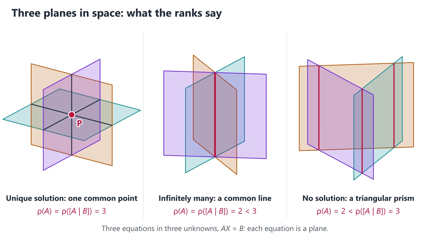
1. Understanding the Augmented Matrix and Row Operations
Why we need it: a system such as 2x + 3y − z = 5, x − y + 4z = 2, ... is long to copy at every step, and the letters x, y, z never change.
Only the numbers change, so we store just the numbers in a rectangle and work on the rectangle.
We also need to know which changes to the equations are safe, that is, which ones keep exactly the same set of solutions.
In words: the coefficient matrix A has one row per equation and one column per unknown; entry aij is the coefficient of the j-th unknown in the i-th equation.
X is the column of unknowns and B is the column of right-hand sides, so the whole system is the single matrix equation AX = B.
The augmented matrix [A | B] is A with the column B written on its right; the bar only reminds us where the equals sign was.
A row of [A | B] is one complete equation, so a row operation is an operation on equations.
There are three elementary row operations: Ri ↔ Rj (swap two equations), Ri → kRi with k ≠ 0 (scale an equation), and Ri → Ri + kRj (add a multiple of one equation to another).
Each of them can be undone by another operation of the same kind, and this reversibility is the whole reason they keep the solution set unchanged.
First example, slowly: take x + 2y = 5 and 3x + 4y = 11.
Step 1: write [A | B] = [[1, 2 | 5], [3, 4 | 11]]; the first row is the first equation, the second row the second equation.
Step 2: to remove x from the second equation, apply R2 → R2 − 3R1; the new second row is (3 − 3, 4 − 6 | 11 − 15) = (0, −2 | −4).
Step 3: read the row back as an equation: 0x − 2y = −4, so y = 2.
Step 4: the first row still says x + 2y = 5, so x = 5 − 4 = 1.
Step 5: check in the original equations: 1 + 4 = 5 and 3 + 8 = 11. Notice that the operation in Step 2 can be undone by R2 → R2 + 3R1, so nothing was lost.
Non-example: adding the x-column of the same system to its right-hand column (a column operation) gives x + 2y = 6, 3x + 4y = 14, whose solution is (2, 2), not (1, 2): column operations that touch B change the problem.
Multiplying a row by k = 0 is also forbidden: it turns an equation into 0 = 0, the step cannot be reversed, and solutions of the other equations that violate the erased one would be wrongly accepted.
Building up: (1) every solution of the old system satisfies the new one, because the new equations are combinations of the old ones.
(2) The reverse operation turns the new system back into the old one, so by the same reasoning every new solution is an old solution.
(3) In matrix language each operation is multiplication on the left by an invertible elementary matrix E, and EAX = EB ⇔ AX = B because E−1 exists.
Where it is used: every later method of this topic (rank test, Gauss elimination, Gauss-Jordan, conditions on a, b, c) is a sequence of these three row operations on [A | B].
2. Matrix Form
A system of m equations in n unknowns is AX = B, with coefficient matrix A (m × n) and augmented matrix [A | B]. It is homogeneous if B = 0.
Idea (row picture): each equation in three unknowns is a plane, and a solution is a point common to all the planes (see the figure above). Column picture: AX = B asks whether B is a combination x1C1 + ... + xnCn of the columns of A, so the system is solvable exactly when B lies in the column space of A.
Equivalent systems: interchanging two equations, multiplying one by k ≠ 0, or adding a multiple of one to another can be reversed, so these row operations on [A | B] never change the solution set. Column operations are not allowed on [A | B], except interchanging two columns of A, which only renames the unknowns.
3. Understanding Rank and Consistency
Why we need it: before solving we want to know whether a solution exists at all, and if so whether it is unique.
Counting equations and unknowns does not answer this, because some equations may repeat information or contradict each other.
The rank measures how many equations are genuinely independent, and comparing two ranks settles the question.
In words: ρ(A) is the number of non-zero rows left after A is reduced to echelon form; it counts the independent left-hand sides.
ρ([A | B]) counts the independent rows when the right-hand sides are included.
Always ρ(A) ≤ ρ([A | B]) ≤ ρ(A) + 1, because adding one column can raise the rank by at most one.
If the two ranks differ, some combination of the equations has left side 0 but right side c ≠ 0, which is the impossible statement 0 = c.
If they are equal to r, the system is consistent, r unknowns are fixed and the other n − r can be chosen freely.
First example, slowly: consider x + y = 2 and 2x + 2y = 5.
Step 1: [A | B] = [[1, 1 | 2], [2, 2 | 5]].
Step 2: R2 → R2 − 2R1 gives the row (0, 0 | 1).
Step 3: in the A-part only one non-zero row remains, so ρ(A) = 1; in the whole matrix two non-zero rows remain, so ρ([A | B]) = 2.
Step 4: the second row reads 0x + 0y = 1, which no (x, y) satisfies, so there is no solution. Geometrically the two lines are parallel.
Step 5: change 5 to 4. Now the second row is (0, 0 | 0), both ranks are 1 < 2 = n, and the solutions are x = 2 − t, y = t for every t: one free parameter, as n − r = 1 predicts.
Non-example: 'more equations than unknowns means no solution' is false: x + y = 2, x − y = 0, 2x + 3y = 5 has three equations in two unknowns and the solution (1, 1), because ρ(A) = ρ([A | B]) = 2.
Likewise 'fewer equations than unknowns means a solution' is false: x + y + z = 1, x + y + z = 2 has no solution.
Building up: (1) AX = x1C1 + ... + xnCn, where Cj are the columns of A, so AX = B is solvable exactly when B is a combination of the columns.
(2) B is such a combination exactly when appending B adds no new independent column, that is, when ρ([A | B]) = ρ(A).
(3) The number of free unknowns is n − r by the rank-nullity theorem applied to X ↦ AX. The full proof is in Standard Proofs, Theorem 7.
Where it is used: every 'discuss the consistency' or 'for what values of λ, μ' question is answered by this comparison of ranks; it also decides basic solutions in Linear Programming.
4. Consistency Theorem (Rouché-Capelli)
AX = B is consistent if and only if ρ(A) = ρ([A | B]).
Idea: ρ(A) = ρ([A | B]) says that adjoining the column B creates no new independent column, that is, B is already in the column space of A. In echelon form an inconsistency appears as a row (0 0 ... 0 | c) with c ≠ 0, the impossible equation 0 = c. Proved in Standard Proofs, Theorem 7.
If ρ(A) = ρ([A | B]) = n, the solution is unique.
If ρ(A) = ρ([A | B]) = r < n, there are infinitely many solutions, expressed in terms of n − r free parameters.
Why n − r parameters: the echelon form has r pivots, so r pivot variables are determined by the others, while the n − r free variables can be given arbitrary values.
If ρ(A) < ρ([A | B]), the system has no solution.
Structure: the general solution = one particular solution + the general solution of AX = 0; the solutions of AX = 0 form a subspace of dimension n − ρ(A).
Why it works: if AX0 = B and AX = B, then A(X − X0) = 0, so X − X0 ∈ N(A); conversely A(X0 + Y) = B for every Y ∈ N(A). So the solution set is the translate X0 + N(A): a point, a line or a plane parallel to the null space, which passes through the origin only when B = 0.
Consequence: a linear system over ℝ or ℂ has no solution, exactly one, or infinitely many, never exactly two; if X1 ≠ X2 are solutions, then X1 + t(X2 − X1) is a solution for every scalar t.
5. Understanding the Solution Set: Particular plus Homogeneous
Why we need it: when a system has infinitely many solutions we cannot list them; we need a short formula that produces every one of them and nothing else.
The answer is: one solution plus all solutions of the homogeneous system with the same A.
In words: the homogeneous system AX = 0 has the same left sides as AX = B but zero right sides.
Its solution set N(A) is called the null space; it always contains X = 0 and is closed under addition and scaling, so it is a subspace of Fn.
A particular solution X0 is any one solution of AX = B, found by giving the free variables any convenient values, usually 0.
The general solution is X = X0 + Y with Y running over N(A); if N(A) has basis Y1, ..., Yn−r, then X = X0 + t1Y1 + ... + tn−rYn−r.
First example, slowly: solve x + y + z = 3, x − y = 0.
Step 1: a particular solution is easy to guess: X0 = (1, 1, 1), since 1 + 1 + 1 = 3 and 1 − 1 = 0.
Step 2: the homogeneous system is x + y + z = 0, x − y = 0. The second gives y = x; then z = −2x.
Step 3: with x = t, N(A) = {t(1, 1, −2)}, a line through the origin; its dimension is 1 = n − r = 3 − 2.
Step 4: the general solution is X = (1, 1, 1) + t(1, 1, −2) = (1 + t, 1 + t, 1 − 2t).
Step 5: check: (1 + t) + (1 + t) + (1 − 2t) = 3 and (1 + t) − (1 + t) = 0 for every t. The solution set is the line through (1, 1, 1) parallel to (1, 1, −2).
Notice that a different particular solution, say (2, 2, −1) (t = 1), gives the same line, only with a shifted parameter.
Non-example: the solution set of a non-homogeneous system is not a subspace: (1, 1, 1) solves x + y + z = 3, but 2(1, 1, 1) = (2, 2, 2) gives 6, and (0, 0, 0) is not a solution at all.
Building up: (1) if AX0 = B and AX = B, subtracting gives A(X − X0) = 0, so every solution differs from X0 by an element of N(A).
(2) Conversely A(X0 + Y) = B + 0 = B for every Y ∈ N(A).
(3) dim N(A) = n − ρ(A) by rank-nullity, so AX = 0 has a non-trivial solution exactly when ρ(A) < n; since ρ(A) ≤ m, this is automatic when m < n.
Where it is used: the same 'particular + homogeneous' structure gives the general solution of a linear ODE (particular integral + complementary function), and eigenvectors are exactly the non-zero vectors of N(A − λI).
6. Homogeneous Systems
AX = 0 always has the trivial solution X = 0. It has a non-trivial solution if and only if ρ(A) < n; for a square system, if and only if det A = 0.
Idea: every plane ax + by + cz = 0 passes through the origin, so X = 0 is always a solution; a non-trivial solution means the planes share at least a whole line through the origin. For a square system det A = 0 ⇔ ρ(A) < n ⇔ at least one free variable.
If m < n (fewer equations than unknowns), a non-trivial solution always exists.
Why it works: ρ(A) ≤ m < n, so at least n − m variables are free and can be given non-zero values.
7. Understanding Gauss Elimination
Why we need it: substitution works for two equations but becomes chaotic for three or more; we need a fixed routine that always ends with the answer, or with a proof that there is none.
In words: a pivot is the first non-zero entry of a row in the reduced matrix; the column it sits in belongs to a pivot variable.
The multiplier for row i is ai1/a11: subtracting that multiple of the pivot row makes the entry below the pivot zero.
Echelon form means: every pivot lies to the right of the pivot in the row above, and zero rows are at the bottom; the matrix looks like a staircase.
Variables without a pivot are free variables; they become the parameters t, s, ... of the answer.
Back-substitution solves the last non-zero equation first and moves upwards.
First example, slowly: solve x + y + z = 4, 2x + 3y + z = 9, x + 3y + 4z = 11.
Step 1: the pivot of column 1 is a11 = 1. R2 → R2 − 2R1 gives (0, 1, −1 | 1); R3 → R3 − R1 gives (0, 2, 3 | 7).
Step 2: the pivot of column 2 is now 1 (row 2). R3 → R3 − 2R2 gives (0, 0, 5 | 5).
Step 3: three pivots, so ρ(A) = ρ([A | B]) = 3 = n: a unique solution, with no free variable.
Step 4: back-substitute: 5z = 5 gives z = 1; y − z = 1 gives y = 2; x + y + z = 4 gives x = 1.
Step 5: check in the third original equation: 1 + 6 + 4 = 11.
With a free variable: x + 2y − z = 1, 2x + 4y + z = 8. R2 − 2R1 gives (0, 0, 3 | 6), so the pivots are in the x- and z-columns and y = t is free; then z = 2 and x = 1 − 2t + 2 = 3 − 2t.
Non-example: for y + z = 1, x + y = 3, x + z = 4 the entry a11 is 0, so it cannot be a pivot and 'R2 − (a21/a11)R1' would divide by zero; first swap R1 ↔ R2.
Building up: (1) each elimination step is a row operation, so the reduced system has the same solutions (lesson on row operations).
(2) In echelon form the ranks are visible as numbers of pivots, so consistency is read off at once.
(3) The echelon system is triangular in the pivot variables, so back-substitution always succeeds, and the free variables can take any values.
Where it is used: the same elimination computes ranks, inverses (Gauss-Jordan on [A | I]), bases of null spaces and eigenvectors, and is the direct method of Numerical Analysis.
8. Methods
Gauss elimination: (1) reduce [A | B] to row echelon form; (2) read the two ranks and decide consistency; (3) assign parameters to the non-pivot (free) variables; (4) back-substitute.
Why back-substitution works: the echelon system is triangular in the pivot variables, so the last non-zero equation gives the last pivot variable in terms of the free ones, and each earlier equation then gives one more pivot variable.
Gauss-Jordan: reduce [A | B] to reduced echelon form and read off the solution directly.
Cramer's rule: if A is n × n with Δ = det A ≠ 0, then xi = Δi/Δ, where Δi is det A with its i-th column replaced by B.
Derivation of Cramer's rule: X = A−1B = (adj A)B/Δ, so xi = (∑jCjibj)/Δ, where Cji is the cofactor of aji. The sum ∑jbjCji is the expansion along column i of the determinant obtained from A by replacing column i with B, that is Δi, hence xi = Δi/Δ.
When Δ = 0: A·adj A = ΔI gives Δxi = Δi for every solution, so if Δ = 0 and some Δi ≠ 0 the system is inconsistent. But Δ = Δ1 = ... = Δn = 0 does not guarantee a solution when n ≥ 3 (for n = 2 it does, unless A is the zero matrix): x + y + z = 1, x + y + z = 2, x + y + z = 3 has all four determinants 0 and no solution.
Inverse method: X = A−1B when A is non-singular.
Systems with parameters: for a square system first find the parameter values with det A = 0; for all other values the solution is unique (Cramer). For each value with det A = 0 reduce [A | B] and compare ρ(A) with ρ([A | B]).
Consistency conditions: to find the condition on the right side (a, b, c) for a solution, keep a, b, c as letters while reducing [A | B]; the entry opposite a zero row of A must vanish.
9. Derivation: Gauss Elimination in Operation Form
Step 1: choose a pivot a11 ≠ 0 in the first column (interchange rows if needed). Step 2: Ri → Ri − (ai1/a11)R1 for i = 2, ..., m clears the first column below the pivot.
Step 3: repeat on the rows below the pivot, moving to the next column whenever a column has no non-zero entry left; stop when no rows remain. Each step is pre-multiplication by an invertible elementary matrix, so with E = Ek...E1 the new system EAX = EB has exactly the same solutions as AX = B.
Reading the ranks: ρ(A) is the number of pivots in the A-part and ρ([A | B]) the number in the whole augmented matrix; they differ (by exactly 1) precisely when a row (0 ... 0 | c), c ≠ 0, appears.
LU form: when no row interchanges are needed, the multipliers ai1/a11, ... placed below the diagonal of I form a unit lower triangular L with A = LU, U being the echelon form; solving LY = B and then UX = Y is the same elimination done in two stages.
10. Geometry of Three Equations in Three Unknowns
Each equation aix + biy + ciz = di is a plane with normal (ai, bi, ci), and ρ(A) is the number of independent normals (see the figure above and the table of ranks in this topic).
ρ(A) = 3: the normals are independent and the three planes meet in exactly one point.
ρ(A) = 2: the normals lie in one plane, so all three planes are parallel to one fixed line. If ρ([A | B]) = 2 they share a common line; if ρ([A | B]) = 3 they form a triangular prism, or two of them are parallel and the third cuts both.
ρ(A) = 1: all three planes are parallel. If ρ([A | B]) = 1 they coincide (a two-parameter family of solutions); if ρ([A | B]) = 2 at least two are distinct parallel planes and there is no solution.
11. Choosing the Method
If A is square and Δ = det A ≠ 0 is easy to see → Cramer's rule (for n ≤ 3) or X = A−1B when A−1 is already known or is also asked.
If the system is not square, or Δ = 0, or consistency must be discussed → Gauss elimination on [A | B] and comparison of the two ranks.
If the coefficients contain a parameter → find the values with det A = 0 first; for all other values the solution is unique, and [A | B] is reduced separately at each special value.
If conditions on the right-hand side (a, b, c) are asked → keep a, b, c as letters in the last column; each zero row of the A-part gives one linear condition.
If the system is homogeneous → only ρ(A) matters; for a square system det A = 0 is the condition for non-trivial solutions, and the answer should be a basis of N(A).
If n is large or the coefficients are decimals → elimination with partial pivoting, or an iterative method such as Gauss-Seidel when A is diagonally dominant (Numerical Analysis).
12. Common Mistakes
Using Cramer's rule when Δ = 0, or concluding 'infinitely many solutions' only because Δ = Δ1 = Δ2 = Δ3 = 0; the ranks must be compared.
Applying column operations to [A | B]; they mix the unknowns with the right-hand side and change the solution set.
Stopping at 'the system is consistent' without writing the general solution in parametric form with exactly n − r parameters.
Dividing by an expression containing the parameter (such as λ − 3) without treating λ = 3 separately.
Answering only X = 0 for a homogeneous system with det A = 0, when a basis of the solution space is expected.
Not substituting the final solution back into the original equations; a one-line check catches most arithmetic slips.
13. Connections
Link: in Linear Programming, a basic solution of AX = B (m equations, rank m) is found by setting n − m variables to 0 and solving for the other m, whose columns must be independent; the simplex method moves from one such solution to another.
Link: eigenvectors are the non-trivial solutions of the homogeneous system (A − λI)X = 0, so the condition det(A − λI) = 0 is exactly the characteristic equation (Eigenvalues).
Link: Gauss elimination, Gauss-Jordan and Gauss-Seidel are the direct and iterative methods of Numerical Analysis; the rank theory here decides when a solution exists before any numerical method is tried.
14. Worked Examples
Example 1: For what values of λ and μ does the system x + y + z = 6, x + 2y + 3z = 10, x + 2y + λz = μ have (i) no solution, (ii) a unique solution, (iii) infinitely many solutions?
R2 − R1 gives y + 2z = 4, and R3 − R2 gives (λ − 3)z = μ − 10.
(i) λ = 3, μ ≠ 10: ρ(A) = 2, ρ([A | B]) = 3, no solution. (ii) λ ≠ 3: ρ(A) = ρ([A | B]) = 3, unique solution. (iii) λ = 3, μ = 10: both ranks are 2, infinitely many solutions.
In case (iii), with z = t: y = 4 − 2t and x = 6 − y − z = 2 + t, so X = (2 + t, 4 − 2t, t), t ∈ ℝ.
Example 2: Find k for which kx + y + z = 0, x + ky + z = 0, x + y + kz = 0 has a non-trivial solution.
det [[k, 1, 1], [1, k, 1], [1, 1, k]] = k3 − 3k + 2 = (k − 1)2(k + 2) = 0, so k = 1 or k = −2.
For k = 1 the system is the single equation x + y + z = 0, a two-parameter family. For k = −2 the rank is 2 and the solution is x = y = z = t.
Example 3 (Cramer): 2x + y = 5, x − y = 1. Δ = −3, Δ1 = det [[5, 1], [1, −1]] = −6, Δ2 = det [[2, 5], [1, 1]] = −3, so x = 2, y = 1.
Example 4: Solve by Gaussian elimination: x + y + z = 6, 2x − y + 3z = 9, x + 2y − z = 2.
R2 − 2R1: −3y + z = −3; R3 − R1: y − 2z = −4.
From the second, y = 2z − 4; substituting, −3(2z − 4) + z = −3, so −5z = −15 and z = 3, y = 2, x = 6 − 2 − 3 = 1. Solution (1, 2, 3); check in the second equation: 2 − 2 + 9 = 9.
Example 5: Find a basis of the solution space of x + 2y − z + w = 0, 2x + 4y + z − w = 0, 3x + 6y = 0.
The third equation is the sum of the first two, and the first two are independent, so ρ(A) = 2 and the solution space has dimension 4 − 2 = 2.
Adding the first two: 3x + 6y = 0, so x = −2y; then the first gives w = z. With y = s, z = t: X = s(−2, 1, 0, 0) + t(0, 0, 1, 1), and these two vectors form a basis.
Example 6: Show that x + 2y + 3z = 1, 2x + 3y + 4z = 2, 3x + 4y + 5z = 4 is inconsistent.
The coefficient rows satisfy R3 = 2R2 − R1, so ρ(A) = 2. The same combination of the right sides gives 2(2) − 1 = 3 ≠ 4.
Hence the reduced augmented matrix has a row (0, 0, 0 | 1), ρ([A | B]) = 3 ≠ ρ(A), and by the Rouché-Capelli theorem there is no solution.
Example 7: For which a is the system x + y + z = 1, x + 2y + 4z = a, x + 4y + 10z = a2 consistent? Solve it in each case.
R2 − R1: y + 3z = a − 1; R3 − R1: 3y + 9z = a2 − 1. Subtracting 3 times the first: 0 = a2 − 3a + 2 = (a − 1)(a − 2).
So ρ(A) = 2 always, and the system is consistent only for a = 1 or a = 2.
a = 1: y = −3k, x = 1 + 2k, z = k. a = 2: y = 1 − 3k, x = 2k, z = k (k ∈ ℝ); check a = 2, k = 0: (0, 1, 0) gives 1, 2, 4.
15. Solved UPSC Questions
Example 8 (UPSC 2016, 10 marks): (i) Using elementary row operations, find the condition that the linear equations
x − 2y + z = a
2x + 7y − 3z = b
3x + 5y − 2z = c
have a solution. (7 marks)
(ii) If
W1 = {(x, y, z) | x + y − z = 0}
W2 = {(x, y, z) | 3x + y − 2z = 0}
W3 = {(x, y, z) | x − 7y + 3z = 0}
then find dim(W1 ∩ W2 ∩ W3) and dim(W1 + W2). (3 marks)
(i) In [A | B], R2 − 2R1 gives (0, 11, −5 | b − 2a) and R3 − 3R1 gives (0, 11, −5 | c − 3a); then R3 − R2 gives (0, 0, 0 | c − a − b).
ρ(A) = 2, so the system is consistent ⇔ ρ([A | B]) = 2 ⇔ c = a + b (then it has infinitely many solutions).
(ii) W1 ∩ W2 ∩ W3 is the solution space of the matrix [[1, 1, −1], [3, 1, −2], [1, −7, 3]]; R2 − 3R1 = (0, −2, 1) and R3 − R1 = (0, −8, 4) = 4(0, −2, 1), so the rank is 2 and the dimension is 3 − 2 = 1 (the line L{(1, 1, 2)}).
W1, W2 are distinct planes through 0 (dimension 2 each) with W1 ∩ W2 = L{(1, 1, 2)}, so dim(W1 + W2) = 2 + 2 − 1 = 3, i.e. W1 + W2 = ℝ3.
Answer: (i) c = a + b; (ii) dim(W1 ∩ W2 ∩ W3) = 1 and dim(W1 + W2) = 3.
Example 9 (UPSC 2019, 10 marks): If
A = [[1, 2, 1], [1, −4, 1], [3, 0, −3]] and B = [[2, 1, 1], [1, −1, 0], [2, 1, −1]]
then show that AB = 6I3. Use this result to solve the following system of equations :
2x + y + z = 5
x − y = 0
2x + y − z = 1
Row 1 of A against the columns of B: (2 + 2 + 2, 1 − 2 + 1, 1 + 0 − 1) = (6, 0, 0); row 2: (2 − 4 + 2, 1 + 4 + 1, 1 + 0 − 1) = (0, 6, 0); row 3: (6 + 0 − 6, 3 + 0 − 3, 3 + 0 + 3) = (0, 0, 6). So AB = 6I3.
Hence B−1 = A/6. The given system is BX = C with C = (5, 0, 1)T, since its coefficient matrix is exactly B.
X = B−1C = (1/6)AC = (1/6)(5 + 0 + 1, 5 − 0 + 1, 15 + 0 − 3) = (1, 1, 2). Check: 2 + 1 + 2 = 5, 1 − 1 = 0, 2 + 1 − 2 = 1.
Answer: x = 1, y = 1, z = 2.
Example 10 (UPSC 2020, 15 marks): Let A = [[1, 0, 2], [2, −1, 3], [4, 1, 8]] and B = [[−11, 2, 2], [−4, 0, 1], [6, −1, −1]].
(i) Find AB.
(ii) Find det(A) and det(B).
(iii) Solve the following system of linear equations : x + 2z = 3, 2x − y + 3z = 3, 4x + y + 8z = 14
(i) Row 1 (1, 0, 2) of A against the columns of B gives (−11 + 12, 2 − 2, 2 − 2) = (1, 0, 0); row 2 (2, −1, 3) gives (−22 + 4 + 18, 4 − 3, 4 − 1 − 3) = (0, 1, 0); row 3 (4, 1, 8) gives (−44 − 4 + 48, 8 − 8, 8 + 1 − 8) = (0, 0, 1). So AB = I.
(ii) det A = 1(−8 − 3) − 0 + 2(2 + 4) = 1, and det A · det B = det(AB) = 1 gives det B = 1.
(iii) The system is AX = C with C = (3, 3, 14)T and A−1 = B, so X = BC = (−33 + 6 + 28, −12 + 0 + 14, 18 − 3 − 14) = (1, 2, 1).
Check: 1 + 2 = 3, 2 − 2 + 3 = 3, 4 + 2 + 8 = 14.
Answer: AB = I, det A = det B = 1, and x = 1, y = 2, z = 1.
16. Practice Exercises
Exercise 1 (basic): Write the augmented matrix of x + 2y = 3, 2x + 4y = 7, find ρ(A) and ρ([A | B]), and decide whether the system is consistent.
Answer: [[1, 2 | 3], [2, 4 | 7]]; R2 − 2R1 = (0, 0 | 1), so ρ(A) = 1, ρ([A | B]) = 2: inconsistent (parallel lines).
Exercise 2 (basic): Is the solution set of x + y − z = 1 a subspace of ℝ3? Is that of x + y − z = 0?
Answer: The first is not (it does not contain 0); the second is, a plane through 0 of dimension 2.
Exercise 3 (basic): A consistent system has 4 equations in 6 unknowns and ρ(A) = 3. How many free parameters does its general solution have, and what is dim N(A)?
Answer: n − r = 6 − 3 = 3 parameters; dim N(A) = 3.
Exercise 4 (standard): Solve by Gauss elimination: x + y + z = 6, x + 2y + 3z = 14, x + 4y + 9z = 36.
Answer: y + 2z = 8, 3y + 8z = 30, then 2z = 6: z = 3, y = 2, x = 1.
Exercise 5 (standard): Find a basis and the dimension of the solution space of x + y + z + w = 0, x + 2y + 3z + 4w = 0.
Answer: y = −2z − 3w, x = z + 2w; basis (1, −2, 1, 0), (2, −3, 0, 1); dimension 2.
Exercise 6 (standard): Discuss, for all real k and m, the system x + y + z = 1, x + 2y − z = 2, 2x + 3y + kz = m, and solve it when it has infinitely many solutions.
Answer: Elimination gives y − 2z = 1 and kz = m − 3. k ≠ 0: unique solution; k = 0, m = 3: infinitely many, (x, y, z) = (−3t, 1 + 2t, t); k = 0, m ≠ 3: no solution.
Exercise 7 (standard): Solve 3x + 2y = 7, x − y = −1 by Cramer's rule.
Answer: Δ = −5, Δ1 = −5, Δ2 = −10, so x = 1, y = 2.
Exercise 8 (UPSC level): Using elementary row operations, find the condition on a, b, c for x + 2y − 3z = a, 2x + 6y − 11z = b, x − 2y + 7z = c to be consistent, and state the number of free parameters then.
Answer: R2 − 2R1 = (0, 2, −5 | b − 2a), R3 − R1 = (0, −4, 10 | c − a), then R3 + 2R2 = (0, 0, 0 | c + 2b − 5a). Consistent ⇔ 5a = 2b + c, with ρ = 2 and one free parameter.
Exercise 9 (UPSC level): Let a, b, c be distinct. Show that x + y + z = 1, ax + by + cz = d, a2x + b2y + c2z = d2 has a unique solution and find x.
Answer: Δ is the Vandermonde determinant (b − a)(c − a)(c − b) ≠ 0; Cramer gives x = (d − b)(d − c)/((a − b)(a − c)), and y, z by cyclic change.
Exercise 10 (UPSC level): Find the real values of λ for which x + 2y + 3z = λx, 3x + y + 2z = λy, 2x + 3y + z = λz has a non-trivial solution, and find that solution.
Answer: det(A − λI) = 0 gives λ3 − 3λ2 − 15λ − 18 = (λ − 6)(λ2 + 3λ + 3) = 0; the quadratic has no real root, so λ = 6, and then ρ = 2 with solution x = y = z = t.
| Condition | Nature of solution | Free parameters |
|---|---|---|
| ρ(A) = ρ([A | B]) = n | Unique solution | 0 |
| ρ(A) = ρ([A | B]) = r < n | Infinitely many solutions | n − r |
| ρ(A) < ρ([A | B]) | Inconsistent (no solution) | — |
| AX = 0 with ρ(A) = n | Only the trivial solution | 0 |
| AX = 0 with ρ(A) = r < n | Non-trivial solutions | n − r |
| ρ(A) | ρ([A | B]) | Position of the three planes | Solutions |
|---|---|---|---|
| 3 | 3 | Meet in a single point | Unique |
| 2 | 2 | Pass through one common line (two may coincide) | One-parameter family |
| 2 | 3 | Triangular prism, or two parallel planes cut by the third | None |
| 1 | 1 | All three coincide | Two-parameter family |
| 1 | 2 | Parallel, at least two of them distinct | None |
Mains points
- The parameter question (find λ, μ for no / unique / infinitely many solutions) is a standard 10-15 mark question; reduce the augmented matrix and discuss all three cases separately.
- Always quote the ranks of A and [A | B] explicitly in each case; a correct answer without ranks loses marks.
- In the infinitely-many case, write the full parametric solution, not just 'infinitely many'.
- For homogeneous systems, find the basis of the solution space and state its dimension n − ρ(A).
- Do not divide by an expression such as (λ − 3) during reduction without first treating the case where it is zero.
Did you know?
- Elimination for linear systems appears in the Chinese text 'Nine Chapters on the Mathematical Art' (around the 1st century CE), about 1,500 years before Gauss.
Eigenvalues, Eigenvectors and the Cayley-Hamilton Theorem
The eigenvalues of A are the roots of the characteristic polynomial det(λI − A); their sum is the trace and their product the determinant. A is diagonalisable exactly when it has n independent eigenvectors. The Cayley-Hamilton theorem (every matrix satisfies its characteristic equation) gives A−1 and high powers of A.
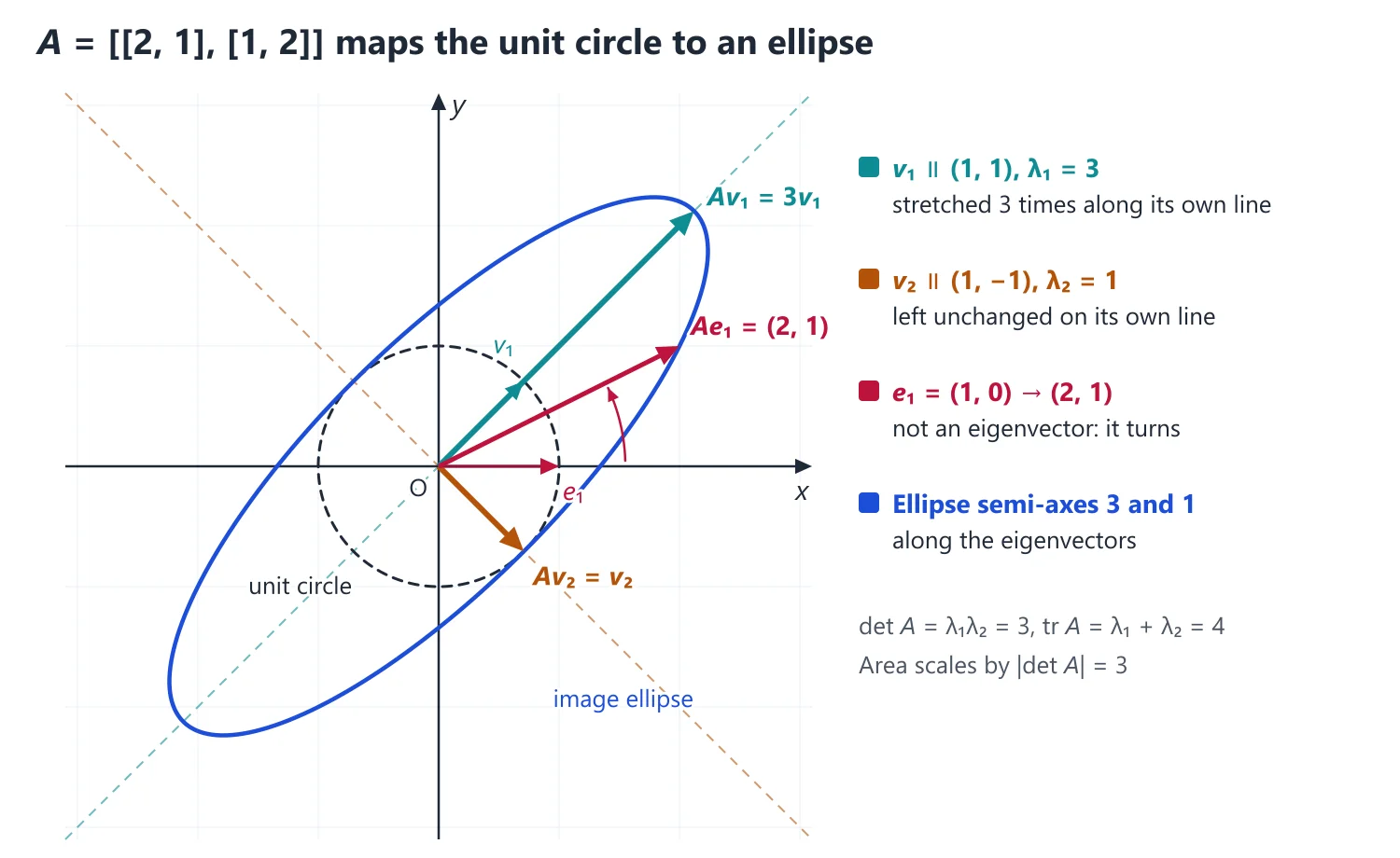
1. Understanding Eigenvalues and Eigenvectors
Why we need it: a matrix A moves almost every vector to a new direction, which makes A2, A10 or eA hard to picture or compute.
If we can find special directions that A only stretches, then on those directions A acts like an ordinary number, and everything becomes simple.
In words: 'AX = λX' says: when A acts on X, the result points along X itself, scaled by the number λ.
'For some non-zero X' is essential: X = 0 satisfies A0 = λ0 for every λ, so it carries no information.
λ is the eigenvalue, the stretch factor; it may be negative (the direction is reversed), zero (the direction is crushed to 0) or, over ℂ, complex.
X is an eigenvector belonging to λ; any non-zero multiple kX is also one, so we really find a whole line (or plane) of eigenvectors.
First example, slowly: let A = [[2, 1], [1, 2]].
Step 1: try X = (1, 1). AX = (2 + 1, 1 + 2) = (3, 3) = 3(1, 1). So X is an eigenvector with λ = 3.
Step 2: try X = (1, −1). AX = (2 − 1, 1 − 2) = (1, −1) = 1·(1, −1). So λ = 1 is another eigenvalue.
Step 3: try X = (1, 0). AX = (2, 1), which is not a multiple of (1, 0), so (1, 0) is not an eigenvector: A turns it.
Step 4: notice that (1, 0) = ½(1, 1) + ½(1, −1); applying A gives ½·3(1, 1) + ½·1(1, −1) = (2, 1). Splitting a vector along eigenvectors turns the action of A into two multiplications.
Non-example: the quarter-turn R = [[0, −1], [1, 0]] sends (x, y) to (−y, x), which is perpendicular to (x, y); no non-zero real vector keeps its direction, so R has no real eigenvalue (its eigenvalues are ±i).
Building up: (1) AX = λX is the same as (A − λI)X = 0, a homogeneous system with the unknown vector X.
(2) A homogeneous square system has a non-zero solution exactly when its determinant is 0, so λ is an eigenvalue ⇔ det(A − λI) = 0.
(3) Once λ is known, the eigenvectors are the non-zero vectors of the null space N(A − λI), found by elimination.
Where it is used: powers and inverses of matrices, systems X′ = AX of differential equations, principal axes of conics and conicoids, and stability of iterations.
2. Understanding the Characteristic Polynomial and Multiplicities
Why we need it: guessing eigenvectors works only for very simple matrices; we need a procedure that finds all eigenvalues of any square matrix.
We also need to count eigenvectors correctly, because that count decides diagonalisation.
In words: p(λ) = det(λI − A) is a polynomial of degree n in the letter λ, with leading coefficient 1; it is called the characteristic polynomial.
Its roots are exactly the eigenvalues, so an n × n matrix has at most n distinct eigenvalues, and over ℂ exactly n counted with multiplicity.
The algebraic multiplicity AM(λ) is how many times λ is repeated as a root of p.
The geometric multiplicity GM(λ) is the number of independent eigenvectors for λ, that is, dim N(A − λI) = n − ρ(A − λI).
First example, slowly: let A = [[4, 1], [2, 3]].
Step 1: λI − A = [[λ − 4, −1], [−2, λ − 3]].
Step 2: p(λ) = (λ − 4)(λ − 3) − (−1)(−2) = λ2 − 7λ + 12 − 2 = λ2 − 7λ + 10.
Step 3: factor: p(λ) = (λ − 2)(λ − 5), so λ = 2 and λ = 5, each with AM = 1.
Step 4: λ = 5: A − 5I = [[−1, 1], [2, −2]], whose rows both say x = y; eigenvector (1, 1), check A(1, 1) = (5, 5).
Step 5: λ = 2: A − 2I = [[2, 1], [2, 1]] gives 2x + y = 0; eigenvector (1, −2), check A(1, −2) = (2, −4).
Step 6: notice that 2 + 5 = 7 = tr A and 2 × 5 = 10 = det A: this is a free check on the arithmetic.
Non-example: for the shear [[3, 1], [0, 3]], p(λ) = (λ − 3)2, so AM(3) = 2, but A − 3I = [[0, 1], [0, 0]] has rank 1 and GM(3) = 1: a repeated root does not guarantee two independent eigenvectors.
Building up: (1) expanding det(λI − A), the λn and λn−1 terms come only from the diagonal product, giving λn − (tr A)λn−1; λ = 0 gives the constant term (−1)ndet A.
(2) Comparing with (λ − λ1)...(λ − λn) gives ∑λi = tr A and ∏λi = det A.
(3) Why GM ≤ AM: take a basis of Eλ (g vectors) and extend it to a basis of Fn; in that basis A becomes [[λIg, *], [0, C]], whose characteristic polynomial (t − λ)gdet(tI − C) already contains (t − λ)g.
Where it is used: every eigenvalue question starts here; for 3 × 3 matrices use the shortcut λ3 − (tr A)λ2 + (sum of principal 2 × 2 minors)λ − det A.
3. Definitions
λ ∈ F is an eigenvalue of the n × n matrix A if AX = λX for some non-zero X; such an X is an eigenvector belonging to λ.
Idea: an eigenvector is a direction that A does not turn: A only stretches it by the factor λ, reversing it when λ < 0. In the figure above a symmetric matrix maps the unit circle to an ellipse; the eigenvectors lie along the axes of the ellipse and the eigenvalues 3 and 1 are the semi-axes, while any other vector is turned.
Why X ≠ 0 is required: A0 = λ0 for every scalar λ, so allowing X = 0 would make every number an eigenvalue.
Characteristic polynomial: p(λ) = det(λI − A) = λn − (tr A)λn−1 + ... + (−1)n det A; the eigenvalues are the roots of p(λ) = 0.
Derivation: AX = λX with X ≠ 0 ⇔ (λI − A)X = 0 has a non-trivial solution ⇔ det(λI − A) = 0. Putting λ = 0 gives the constant term p(0) = det(−A) = (−1)ndet A. The λn−1 term comes only from (λ − a11)(λ − a22)...(λ − ann), because every other term of the expansion misses at least two diagonal entries, so its coefficient is −(a11 + ... + ann) = −tr A.
For a 3 × 3 matrix: λ3 − (tr A)λ2 + (sum of the principal 2 × 2 minors)λ − det A = 0.
Eigenspace Eλ = N(A − λI). Algebraic multiplicity (AM) = multiplicity of λ as a root; geometric multiplicity (GM) = dim Eλ = n − ρ(A − λI); always 1 ≤ GM ≤ AM.
Idea: AM counts how often λ occurs as a root and GM counts how many independent directions are actually stretched by λ. For the shear [[2, 1], [0, 2]], λ = 2 has AM = 2 but GM = 2 − ρ([[0, 1], [0, 0]]) = 1 (only the x-direction), so the shear is not diagonalisable.
4. Properties
Sum of the eigenvalues = tr A; product = det A; A is singular ⇔ 0 is an eigenvalue.
Why it works: over ℂ, p(λ) = (λ − λ1)(λ − λ2)...(λ − λn); comparing the λn−1 and constant terms with those found above gives λ1 + ... + λn = tr A and λ1λ2...λn = det A (eigenvalues counted with multiplicity).
If λ is an eigenvalue of A, then λk is one of Ak, 1/λ of A−1 (λ ≠ 0), λ − k of A − kI, f(λ) of f(A) for any polynomial f, and (det A)/λ of adj A (A non-singular).
Why it works: AX = λX gives A2X = A(λX) = λ2X, and by induction AkX = λkX; adding multiples gives f(A)X = f(λ)X. Multiplying AX = λX by A−1 gives A−1X = (1/λ)X, and adj A = (det A)A−1 gives adj A·X = ((det A)/λ)X. The eigenvector X is the same in every case.
A and AT have the same eigenvalues; a triangular or diagonal matrix has its diagonal entries as eigenvalues; similar matrices have the same eigenvalues.
Eigenvectors belonging to distinct eigenvalues are linearly independent.
Proved in Standard Proofs, Theorem 8. Idea: different stretch factors cannot be produced by one combined direction, so each new eigenvalue contributes a genuinely new direction.
Eigenvalues of a linear operator: the eigenvalues of T: V → V are those of its matrix [T] in any basis (all such matrices are similar); X is an eigenvector of [T] exactly when the vector with coordinates X is an eigenvector of T, for example a polynomial when V = Pn.
Rotation: Rθ = [[cos θ, −sin θ], [sin θ, cos θ]] has eigenvalues e±iθ = cos θ ± i sin θ, which are real only for θ = kπ. Nilpotent matrices have only the eigenvalue 0, idempotent ones only 0 and 1, involutory ones only ±1.
5. Understanding Diagonalisation
Why we need it: a diagonal matrix D = diag(d1, ..., dn) is trivial to handle: Dk = diag(d1k, ..., dnk).
Diagonalisation asks whether a change of coordinates makes A diagonal, so that every question about A becomes a question about numbers.
In words: 'A is diagonalisable' means there is an invertible P with P−1AP = D diagonal.
P is the change-of-basis matrix: its columns are the new basis vectors, and they must be eigenvectors of A.
D lists the eigenvalues in the same order as the columns of P.
'Invertible P' means the n eigenvectors must be linearly independent; this is the only real condition.
First example, slowly: continue with A = [[4, 1], [2, 3]], eigenvalues 5, 2, eigenvectors (1, 1), (1, −2).
Step 1: put the eigenvectors as columns: P = [[1, 1], [1, −2]]; det P = −3 ≠ 0, so P is invertible.
Step 2: in the same order, D = diag(5, 2).
Step 3: check AP = PD column by column: A(1, 1) = 5(1, 1) and A(1, −2) = 2(1, −2), which are exactly the columns of PD.
Step 4: P−1 = (1/3)[[2, 1], [1, −1]], and An = PDnP−1 = (1/3)[[2·5n + 2n, 5n − 2n], [2·5n − 2·2n, 5n + 2·2n]].
Step 5: check n = 1: (1/3)[[12, 3], [6, 9]] = [[4, 1], [2, 3]] = A. Always test the final formula at n = 1.
Non-example: the shear [[1, 1], [0, 1]] has the single eigenvalue 1 and only the eigenvectors k(1, 0); two independent eigenvectors do not exist, so no invertible P works and the matrix is not diagonalisable.
Building up: (1) AP = PD read column by column says AXj = λjXj, so the columns of P must be eigenvectors (Standard Proofs, Theorem 10).
(2) Eigenvectors of distinct eigenvalues are independent (Theorem 8), so n distinct eigenvalues always suffice.
(3) With repeated eigenvalues, the bases of the eigenspaces together are independent, so we get n of them exactly when GM = AM for every eigenvalue (and all eigenvalues lie in the field).
Where it is used: An, eAt for X′ = AX, Markov chains, and the reduction of quadratic forms and conicoids to principal axes.
6. Diagonalisation
A is diagonalisable (P−1AP = D) if and only if A has n linearly independent eigenvectors, if and only if all its eigenvalues lie in F (automatic over ℂ) and GM = AM for every eigenvalue; P has the eigenvectors as columns and D has the eigenvalues in the same order.
Derivation: if AXi = λiXi and P = [X1 X2 ... Xn] (eigenvectors as columns), then AP = [λ1X1 ... λnXn] = PD. P is invertible exactly when the Xi are independent, and then P−1AP = D; the criterion GM = AM is proved in Standard Proofs, Theorem 10.
Idea: in a basis of eigenvectors the operator simply scales each coordinate axis by its own factor, which is why powers, inverses and functions of A become easy.
n distinct eigenvalues ⇒ diagonalisable (sufficient, not necessary). Then Ak = PDkP−1.
Why Ak = PDkP−1: A = PDP−1 gives Ak = (PDP−1)(PDP−1)...(PDP−1) = PDkP−1, since each inner P−1P cancels; similarly f(A) = Pf(D)P−1 for any polynomial or power series f, such as eA.
Minimal polynomial m(λ): the monic polynomial of least degree with m(A) = 0; it divides p(λ), has the same distinct roots, and, over ℂ, A is diagonalisable if and only if m(λ) has no repeated roots (over ℝ its roots must also all be real).
Why m divides p: write p(λ) = q(λ)m(λ) + r(λ) with deg r < deg m; then r(A) = p(A) − q(A)m(A) = 0, so r = 0 by the minimality of m. Every eigenvalue is a root of m, because m(A)X = m(λ)X = 0 with X ≠ 0.
Example: the shear [[2, 1], [0, 2]] has m(λ) = (λ − 2)2, a repeated root, so it is not diagonalisable, while 2I has the same characteristic polynomial but m(λ) = λ − 2.
7. Understanding the Cayley-Hamilton Theorem
Why we need it: computing A−1 by cofactors or A50 by repeated multiplication is long; we want to replace high powers of A by low ones.
The theorem gives one polynomial equation that A always obeys, of degree n, and that is enough to reduce every power of A to degree at most n − 1.
In words: write p(λ) = λn + c1λn−1 + ... + cn; 'A satisfies p' means that replacing λk by Ak and the constant cn by cnI gives the zero matrix.
The I is needed because a number cannot be added to a matrix.
First example, slowly: for A = [[4, 1], [2, 3]], p(λ) = λ2 − 7λ + 10.
Step 1: A2 = [[16 + 2, 4 + 3], [8 + 6, 2 + 9]] = [[18, 7], [14, 11]].
Step 2: A2 − 7A + 10I = [[18 − 28 + 10, 7 − 7], [14 − 14, 11 − 21 + 10]] = [[0, 0], [0, 0]]: the theorem is verified.
Step 3: rewrite as A(7I − A) = 10I, so A−1 = (7I − A)/10 = (1/10)[[3, −1], [−2, 4]].
Step 4: check: A·(1/10)[[3, −1], [−2, 4]] = (1/10)[[12 − 2, −4 + 4], [6 − 6, −2 + 12]] = I.
Step 5: powers: A2 = 7A − 10I, so A3 = 7A2 − 10A = 7(7A − 10I) − 10A = 39A − 70I; every power is a combination of A and I.
Non-example: a polynomial other than p need not be satisfied: A2 − 5A + 6I = [[4, 2], [4, 2]] ≠ 0 for the same A. Also, 'p(A) = det(AI − A) = det 0 = 0' is not a proof, because inside the determinant λ is a number, and putting a matrix there produces a matrix with matrix entries.
Building up: (1) for a diagonalisable A = PDP−1, p(A) = Pp(D)P−1 and p(D) = diag(p(λ1), ..., p(λn)) = 0, so the theorem is easy in that case.
(2) For a general A, use (λI − A)·adj(λI − A) = p(λ)I, expand adj(λI − A) in powers of λ with matrix coefficients, compare coefficients and add with weights An, ..., I; everything telescopes to p(A) = 0 (Standard Proofs, Theorem 11).
(3) Since p(A) = 0, the minimal polynomial m(λ) divides p(λ), and dividing λk by p(λ) gives Ak as the remainder evaluated at A.
Where it is used: 'verify Cayley-Hamilton and find A−1', 'express a polynomial in A as a linear polynomial', high powers A30, A100 by a recurrence, and the minimal polynomial.
8. Cayley-Hamilton Theorem
Statement: every square matrix satisfies its own characteristic equation: if p(λ) = det(λI − A), then p(A) = 0.
Proved in Standard Proofs, Theorem 11. Idea: on an eigenvector p(A)X = p(λ)X = 0 is obvious; the theorem says that p(A) kills every vector, including those that are not eigenvectors, even when A is not diagonalisable.
Uses: (1) inverse: if An + c1An−1 + ... + cnI = 0 with cn = (−1)ndet A ≠ 0, then A−1 = −(An−1 + c1An−2 + ... + cn−1I)/cn; (2) high powers: divide λm by p(λ) and evaluate the remainder at A.
Derivation of the inverse formula: move cnI to the right: A(An−1 + c1An−2 + ... + cn−1I) = −cnI, and divide by −cn ≠ 0; the bracket divided by −cn is A−1.
Derivation for powers: λm = q(λ)p(λ) + r(λ) with deg r ≤ n − 1 gives Am = q(A)p(A) + r(A) = r(A). The n coefficients of r are found by putting each eigenvalue into λm = r(λ), and, at an eigenvalue of multiplicity k, also the first k − 1 derivatives mλm−1 = r′(λ), ....
The argument 'p(A) = det(AI − A) = 0' is not a proof, because λ is a scalar inside the determinant; the standard proof uses (λI − A)·adj(λI − A) = p(λ)I.
High powers by a recurrence: when p(λ) has a convenient form, rewrite p(A) = 0 as A3 = (lower powers), multiply by An−3 and prove the resulting recurrence by induction; for example λ3 − λ2 − λ + 1 gives An = An−2 + A2 − I.
9. Choosing the Method
If the eigenvalues of a 3 × 3 matrix are needed → write λ3 − (tr A)λ2 + (sum of principal 2 × 2 minors)λ − det A = 0 and, for integer entries, try the integer divisors of det A as roots.
If diagonalisability is asked → find the AM of each eigenvalue, compute GM = n − ρ(A − λI) for each repeated eigenvalue, and use: diagonalisable ⇔ GM = AM for all eigenvalues (or ⇔ m(λ) has no repeated root).
If a high power Ak is asked → PDkP−1 when A is diagonalisable with simple eigenvectors; otherwise Cayley-Hamilton with a remainder r(λ) of degree ≤ n − 1, or a recurrence when p(λ) has a neat form.
If A−1 or a polynomial in A is asked 'using the Cayley-Hamilton theorem' → first verify p(A) = 0 by computing A2, A3 (this step carries marks), then reduce.
If the eigenvalues of A2, A−1, adj A, A + kI or f(A) are asked → do not recompute any determinant; use the table of related matrices in this topic, with the same eigenvectors.
If the minimal polynomial is asked → start from ∏(λ − λi) over the distinct eigenvalues and raise exponents one at a time, testing each candidate at A, until the product vanishes.
10. Common Mistakes
Giving the zero vector as an eigenvector, or giving one eigenvector without stating that every non-zero multiple (every non-zero vector of the eigenspace) also qualifies.
Deciding GM by the number of eigenvectors one happened to find instead of computing n − ρ(A − λI).
Ordering mismatch: the k-th column of P must be an eigenvector for the k-th diagonal entry of D.
Assuming that a repeated eigenvalue rules out diagonalisation; 2I has the repeated eigenvalue 2 and is already diagonal.
Writing A2 − 5A + 6 = 0 instead of A2 − 5A + 6I = 0, or 'proving' Cayley-Hamilton by substituting λ = A in det(λI − A).
Taking the eigenvalues of A + B or AB to be sums or products of those of A and B; this is false in general (it holds when A and B commute and are simultaneously diagonalisable).
11. Connections
Link: reducing a central conicoid ax2 + by2 + cz2 + 2fyz + 2gzx + 2hxy = 1 to its principal axes means diagonalising its symmetric matrix: the eigenvalues are the coefficients of the canonical form and the eigenvectors give the principal directions (Analytic Geometry).
Link: the system X′ = AX has solutions eλtV with AV = λV, so for diagonalisable A the general solution is ∑cieλitVi (Ordinary Differential Equations).
Link: the auxiliary equation of the constant-coefficient ODE y″ + a y′ + b y = 0 is the characteristic equation of its companion matrix [[0, 1], [−b, −a]], namely λ2 + aλ + b = 0.
12. Worked Examples
Example 1: Find the eigenvalues and eigenvectors of A = [[2, 2, 1], [1, 3, 1], [1, 2, 2]]. Is A diagonalisable?
tr A = 7, sum of principal minors = 4 + 3 + 4 = 11, det A = 5, so λ3 − 7λ2 + 11λ − 5 = (λ − 1)2(λ − 5) = 0 and λ = 1, 1, 5.
λ = 5: (A − 5I)X = 0 gives X = k(1, 1, 1). λ = 1: every row of A − I is (1, 2, 1), rank 1, so x + 2y + z = 0, with independent eigenvectors (−2, 1, 0) and (−1, 0, 1).
GM(1) = 2 = AM(1), so A is diagonalisable, with P = [[1, −2, −1], [1, 1, 0], [1, 0, 1]] and D = diag(5, 1, 1).
Example 2: Verify the Cayley-Hamilton theorem for A = [[1, 0, 2], [0, −1, 1], [0, 1, 0]] and find A−1.
det(λI − A) = (λ − 1)(λ2 + λ − 1) = λ3 − 2λ + 1, so the theorem claims A3 − 2A + I = 0.
A2 = [[1, 2, 2], [0, 2, −1], [0, −1, 1]] and A3 = [[1, 0, 4], [0, −3, 2], [0, 2, −1]]; then A3 − 2A + I = 0 holds entry by entry.
Multiplying by A−1: A2 − 2I + A−1 = 0, so A−1 = 2I − A2 = [[1, −2, −2], [0, 0, 1], [0, 1, 1]].
Example 3: Diagonalise A = [[1, 1, −2], [−1, 2, 1], [0, 1, −1]].
tr A = 2, sum of principal minors = 3 − 1 − 3 = −1, det A = −2, so λ3 − 2λ2 − λ + 2 = (λ − 1)(λ − 2)(λ + 1) = 0 and λ = 1, 2, −1 (distinct, so A is diagonalisable).
λ = 1: y = 2z, x = 3z, X1 = (3, 2, 1). λ = 2: x = z, y = 3z, X2 = (1, 3, 1). λ = −1: y = 0, x = z, X3 = (1, 0, 1). Check AX2 = (2, 6, 2).
P = [[3, 1, 1], [2, 3, 0], [1, 1, 1]] (det P = 6 ≠ 0) and P−1AP = diag(1, 2, −1).
Example 4: Show that A = [[2, 1, 0], [0, 2, 1], [0, 0, 2]] is not diagonalisable and find its minimal polynomial.
A is triangular, so λ = 2 with AM 3. A − 2I = [[0, 1, 0], [0, 0, 1], [0, 0, 0]] has rank 2, so GM = 3 − 2 = 1 ≠ 3: not diagonalisable.
The minimal polynomial is (λ − 2)k with k ≤ 3; (A − 2I)2 = [[0, 0, 1], [0, 0, 0], [0, 0, 0]] ≠ 0, so m(λ) = (λ − 2)3, which has a repeated root, confirming the result.
Example 5: For A = [[1, 2], [2, 1]], find An using the Cayley-Hamilton theorem.
p(λ) = λ2 − 2λ − 3, roots 3 and −1. Write λn = q(λ)p(λ) + aλ + b; since p(A) = 0, An = aA + bI.
Putting λ = 3 and λ = −1: 3n = 3a + b and (−1)n = −a + b, so a = (3n − (−1)n)/4 and b = (3n + 3(−1)n)/4.
Check n = 2: a = 2, b = 3, and 2A + 3I = [[5, 4], [4, 5]] = A2.
Example 6: For A = [[1, 4], [2, 3]], express A5 − 4A4 − 7A3 + 11A2 − A − 10I as a linear polynomial in A.
p(λ) = λ2 − 4λ − 5, so A2 − 4A − 5I = 0.
Long division: λ5 − 4λ4 − 7λ3 + 11λ2 − λ − 10 = (λ2 − 4λ − 5)(λ3 − 2λ + 3) + (λ + 5).
Replacing λ by A, the first term vanishes, so the expression equals A + 5I = [[6, 4], [2, 8]].
Example 7: Prove or disprove: if λ is an eigenvalue of A and μ is an eigenvalue of B, then λ + μ is an eigenvalue of A + B.
False. A = [[1, 0], [0, 0]] has eigenvalue 1 and B = [[0, 0], [0, 1]] has eigenvalue 1, but A + B = I has only the eigenvalue 1, not 2.
The statement holds when λ and μ share an eigenvector X: (A + B)X = (λ + μ)X.
13. Solved UPSC Questions
Example 8 (UPSC 2023, 20 marks): Let A = [[1, 0, 0], [1, 0, 1], [0, 1, 0]]
(i) Verify the Cayley-Hamilton theorem for the matrix A.
(ii) Show that An = An−2 + A2 − I for n ≥ 3, where I is the identity matrix of order 3. Hence, find A40. (10+10)
(i) λI − A = [[λ − 1, 0, 0], [−1, λ, −1], [0, −1, λ]]; expanding along the first row, det(λI − A) = (λ − 1)(λ2 − 1) = λ3 − λ2 − λ + 1.
A2 = [[1, 0, 0], [1, 1, 0], [1, 0, 1]] and A3 = A·A2 = [[1, 0, 0], [2, 0, 1], [1, 1, 0]]. Entry by entry, A3 − A2 − A + I = 0, which verifies the theorem.
(ii) The theorem gives A3 = A2 + A − I, which is the claim for n = 3. If An = An−2 + A2 − I, then An+1 = An−1 + A3 − A = An−1 + (A2 + A − I) − A = An−1 + A2 − I; by induction the relation holds for all n ≥ 3.
For even powers, A2k = A2k−2 + (A2 − I) = ... = A2 + (k − 1)(A2 − I) = kA2 − (k − 1)I = [[1, 0, 0], [k, 1, 0], [k, 0, 1]].
Answer: A40 = 20A2 − 19I = [[1, 0, 0], [20, 1, 0], [20, 0, 1]].
Example 9 (UPSC 2015, 12 marks): If matrix A = [[1, 0, 0], [1, 0, 1], [0, 1, 0]] then find A30.
This is the matrix of the previous example: its characteristic polynomial is λ3 − λ2 − λ + 1, so by Cayley-Hamilton A3 = A2 + A − I, and by induction An = An−2 + A2 − I for n ≥ 3.
Applying the recurrence 14 times from A30 down to A2: A30 = A2 + 14(A2 − I) = 15A2 − 14I, with A2 = [[1, 0, 0], [1, 1, 0], [1, 0, 1]].
Answer: A30 = [[1, 0, 0], [15, 1, 0], [15, 0, 1]].
Example 10 (UPSC 2019, 15 marks): State the Cayley-Hamilton theorem. Use this theorem to find A100, where
A = [[1, 0, 0], [1, 0, 1], [0, 1, 0]]
Cayley-Hamilton theorem: every square matrix satisfies its characteristic equation; if det(λI − A) = λn + c1λn−1 + ... + cn, then An + c1An−1 + ... + cnI = 0.
Here det(λI − A) = λ3 − λ2 − λ + 1, so A3 = A2 + A − I and (multiplying by An−3 and inducting) An = An−2 + A2 − I for n ≥ 3.
Hence A2k = kA2 − (k − 1)I, and with k = 50, A100 = 50A2 − 49I.
Answer: A100 = [[1, 0, 0], [50, 1, 0], [50, 0, 1]].
Example 11 (UPSC 2022, 15 marks): Find a linear map T : ℝ2 → ℝ2 which rotates each vector of ℝ2 by an angle θ. Also, prove that for θ = π/2, T has no eigenvalue in ℝ.
Write (x, y) = (r cos φ, r sin φ). Rotation by θ sends it to (r cos(φ + θ), r sin(φ + θ)) = (x cos θ − y sin θ, x sin θ + y cos θ).
So T(x, y) = (x cos θ − y sin θ, x sin θ + y cos θ); it is linear, with matrix Rθ = [[cos θ, −sin θ], [sin θ, cos θ]] in the standard basis. Its characteristic equation is λ2 − 2λ cos θ + 1 = 0, with roots cos θ ± i sin θ.
For θ = π/2, T(x, y) = (−y, x) and the equation is λ2 + 1 = 0, with no real root. Directly: T(x, y) = λ(x, y) means −y = λx and x = λy, so x = −λ2x and y = −λ2y; for (x, y) ≠ (0, 0) this needs λ2 = −1, impossible for real λ.
Answer: T(x, y) = (x cos θ − y sin θ, x sin θ + y cos θ); for θ = π/2 the eigenvalues are ±i, so T has no real eigenvalue (no non-zero vector keeps its direction under a quarter-turn).
Example 12 (UPSC 2024, 20 marks): Let A = [[3, 2, 4], [2, 0, 2], [4, 2, 3]] be a 3×3 matrix. Find the eigenvalues and the corresponding eigenvectors of A. Hence find the eigenvalues and the corresponding eigenvectors of A−15, where A−15 = (A−1)15.
tr A = 6; principal minors (0 − 4) + (9 − 16) + (0 − 4) = −15; det A = 3(0 − 4) − 2(6 − 8) + 4(4 − 0) = 8. So λ3 − 6λ2 − 15λ − 8 = (λ − 8)(λ + 1)2 = 0, and λ = 8, −1, −1.
λ = 8: A − 8I = [[−5, 2, 4], [2, −8, 2], [4, 2, −5]]; the first two rows give X = k(2, 1, 2). Check: A(2, 1, 2) = (16, 8, 16).
λ = −1: A + I = [[4, 2, 4], [2, 1, 2], [4, 2, 4]] has rank 1, so the eigenvectors are the non-zero solutions of 2x + y + 2z = 0, a plane with basis (1, −2, 0), (0, −2, 1).
If AX = λX with λ ≠ 0, then X = λA−1X, so A−1X = λ−1X and A−15X = λ−15X. So A−15 has the same eigenvectors, with eigenvalues 8−15 = 2−45 and (−1)−15 = −1 (twice).
Answer: A: λ = 8 with k(2, 1, 2); λ = −1 (twice) with a(1, −2, 0) + b(0, −2, 1). A−15: λ = 2−45 with k(2, 1, 2); λ = −1 (twice) with the same plane of eigenvectors.
Example 13 (UPSC 2025, 20 marks): (i) Find the eigenvalues and the corresponding eigenvectors of the matrix
A = [[1, 2, 0], [2, 1, −6], [2, −2, 3]]. (12 marks)
(ii) Let Pn denote the vector space of all polynomials of degree ≤ n over ℝ. Verify that
dim(P4/P2) = dim P4 − dim P2. (8 marks)
(i) tr A = 5; principal minors (1 − 4) + (3 − 0) + (3 − 12) = −9; det A = 1(3 − 12) − 2(6 + 12) = −45. So λ3 − 5λ2 − 9λ + 45 = (λ − 5)(λ2 − 9) = 0, and λ = 5, 3, −3.
λ = 5: −4x + 2y = 0 and 2x − 4y − 6z = 0 give y = 2x, z = −x, X1 = (1, 2, −1). λ = 3: −2x + 2y = 0 and 2x − 2y − 6z = 0 give y = x, z = 0, X2 = (1, 1, 0).
λ = −3: 4x + 2y = 0 and 2x + 4y − 6z = 0 give y = −2x, z = −x, X3 = (1, −2, −1). Check: AX1 = (1 + 4, 2 + 2 + 6, 2 − 4 − 3) = (5, 10, −5) = 5X1.
(ii) dim P4 = 5 and dim P2 = 3. In P4/P2, p + P2 = q + P2 ⇔ p − q ∈ P2, so each coset is (a3x3 + a4x4) + P2 = a3(x3 + P2) + a4(x4 + P2).
These two cosets are independent: a3x3 + a4x4 ∈ P2 forces a3 = a4 = 0. So dim(P4/P2) = 2 = 5 − 3 = dim P4 − dim P2.
Answer: (i) λ = 5, 3, −3 with eigenvectors k(1, 2, −1), k(1, 1, 0), k(1, −2, −1); (ii) basis {x3 + P2, x4 + P2}, so both sides equal 2.
Example 14 (UPSC 2026, 20 marks): Let T : P2[x] → P2[x] be a linear transformation defined by
T(a0 + a1x + a2x2) = −(a0 + 2a1 + a2) + (2a0 + 3a1)x − 2(a0 + a1)x2
where P2[x] denotes the set of all polynomials in x of degree ≤ 2 and a0, a1, a2 ∈ ℝ. Find the eigenvalues and corresponding eigenvectors of T using the matrix representation of T with respect to the standard basis of P2[x].
T(1) = −1 + 2x − 2x2, T(x) = −2 + 3x − 2x2, T(x2) = −1, so in the basis {1, x, x2}, [T] = [[−1, −2, −1], [2, 3, 0], [−2, −2, 0]] (columns are the coordinates of the images).
tr = 2; principal minors (−3 + 4) + (0 − 2) + 0 = −1; det = −1·det [[2, 3], [−2, −2]] = −2 (third column). So λ3 − 2λ2 − λ + 2 = (λ − 1)(λ + 1)(λ − 2) = 0, and λ = 1, −1, 2.
λ = 1: −2a0 − 2a1 − a2 = 0 and 2a0 + 2a1 = 0 give a1 = −a0, a2 = 0: eigenvector 1 − x.
λ = −1: −2a1 − a2 = 0 and 2a0 + 4a1 = 0 give a2 = −2a1, a0 = −2a1; with a1 = −1, eigenvector 2 − x + 2x2.
λ = 2: −3a0 − 2a1 − a2 = 0 and 2a0 + a1 = 0 give a1 = −2a0, a2 = a0: eigenvector 1 − 2x + x2. Check: T(1 − x) = −(1 − 2) + (2 − 3)x − 2(0)x2 = 1 − x.
Answer: λ = 1: k(1 − x); λ = −1: k(2 − x + 2x2); λ = 2: k(1 − x)2 (k ≠ 0).
14. Practice Exercises
Exercise 1 (basic): Show that (1, 2) is an eigenvector of A = [[1, 2], [2, 4]] and find its eigenvalue. Find the other eigenvalue without solving a quadratic.
Answer: A(1, 2) = (5, 10) = 5(1, 2), λ = 5; tr A = 5 gives the other λ = 0 (det A = 0), with eigenvector (2, −1).
Exercise 2 (basic): Write down the eigenvalues, trace and determinant of [[2, 5, −1], [0, −3, 4], [0, 0, 7]] without expanding any determinant.
Answer: Triangular, so λ = 2, −3, 7; trace 6, determinant −42.
Exercise 3 (basic): A 3 × 3 matrix A has eigenvalues 1, 2, 3. Find det A and the eigenvalues of A2, A−1, adj A and A − 2I.
Answer: det A = 6; A2: 1, 4, 9; A−1: 1, 1/2, 1/3; adj A: 6, 3, 2; A − 2I: −1, 0, 1.
Exercise 4 (standard): Find the eigenvalues and eigenvectors of [[5, 4], [1, 2]].
Answer: λ2 − 7λ + 6 = 0, λ = 6 with k(4, 1) and λ = 1 with k(1, −1), k ≠ 0.
Exercise 5 (standard): Is A = [[1, 1, 1], [0, 2, 1], [0, 0, 1]] diagonalisable? If so, find P and D.
Answer: λ = 1, 1, 2; A − I = [[0, 1, 1], [0, 1, 1], [0, 0, 0]] has rank 1, so GM(1) = 2 = AM(1): diagonalisable. Eigenvectors (1, 0, 0), (0, 1, −1) for 1 and (1, 1, 0) for 2; P = [[1, 0, 1], [0, 1, 1], [0, −1, 0]], D = diag(1, 1, 2).
Exercise 6 (standard): Verify the Cayley-Hamilton theorem for A = [[1, 2, 0], [2, −1, 0], [0, 0, −1]] and use it to find A−1.
Answer: p(λ) = (λ2 − 5)(λ + 1) = λ3 + λ2 − 5λ − 5; A2 = [[5, 0, 0], [0, 5, 0], [0, 0, 1]]; A−1 = (A2 + A − 5I)/5 = (1/5)[[1, 2, 0], [2, −1, 0], [0, 0, −5]].
Exercise 7 (standard): Find the minimal polynomials of A = diag(2, 2, 3) and of B = [[2, 1, 0], [0, 2, 0], [0, 0, 3]]. Which of them is diagonalisable?
Answer: mA = (λ − 2)(λ − 3), A diagonalisable; mB = (λ − 2)2(λ − 3) since (B − 2I)(B − 3I) ≠ 0, so B is not diagonalisable.
Exercise 8 (UPSC level): Diagonalise A = [[3, −1], [−1, 3]] and hence find An.
Answer: λ = 2 with (1, 1), λ = 4 with (1, −1); An = (1/2)[[2n + 4n, 2n − 4n], [2n − 4n, 2n + 4n]].
Exercise 9 (UPSC level): Find the characteristic and minimal polynomials of A = [[1, 2, 2], [2, 1, 2], [2, 2, 1]] and use the minimal polynomial to express A4 as aA + bI.
Answer: p(λ) = (λ − 5)(λ + 1)2; A is symmetric, hence diagonalisable, so m(λ) = (λ − 5)(λ + 1) and A2 = 4A + 5I; then A4 = 104A + 105I (check on λ = 5: 625 = 520 + 105).
Exercise 10 (UPSC level): Let T: P2 → P2, T(p) = (x + 1)p′(x). Find the matrix of T in the basis {1, x, x2}, its eigenvalues and eigenvectors.
Answer: T(1) = 0, T(x) = 1 + x, T(x2) = 2x + 2x2, so [T] = [[0, 1, 0], [0, 1, 2], [0, 0, 2]]; λ = 0, 1, 2 with eigenvectors 1, 1 + x, (1 + x)2.
Exercise 11 (UPSC level): Prove that if A is invertible, then AB and BA have the same characteristic polynomial, hence the same eigenvalues.
Answer: BA = A−1(AB)A, so BA is similar to AB, and similar matrices have the same characteristic polynomial (Standard Proofs, Theorem 9).
| Matrix | Eigenvalue | Eigenvector |
|---|---|---|
| Ak | λk | X |
| A−1 | 1/λ | X |
| kA | kλ | X |
| A − kI | λ − k | X |
| f(A), f a polynomial | f(λ) | X |
| adj A (A non-singular) | (det A)/λ | X |
| AT | λ | In general different |
| P−1AP | λ | P−1X |
Mains points
- Almost every year: find eigenvalues and eigenvectors of a 3 × 3 matrix and decide diagonalisability; give P and D and state P−1AP = D.
- Cayley-Hamilton questions ask to verify the theorem, then find A−1 or a polynomial in A such as A8 − 5A7 + ...; reduce using p(A) = 0 rather than multiplying out.
- For repeated eigenvalues, compute ρ(A − λI) to get GM; this decides diagonalisability and earns the marks.
- Check the characteristic polynomial with tr A and det A before finding eigenvectors; an early arithmetic slip ruins the whole question.
- Questions on the minimal polynomial: test the divisors of p(λ) with the same distinct roots in increasing degree.
Did you know?
- Cayley stated the theorem in 1858 but checked it only for 2 × 2 and 3 × 3 matrices; the first general proof was given by Frobenius in 1878.
Symmetric, Hermitian, Orthogonal and Unitary Matrices and Their Eigenvalues
Hermitian (and real symmetric) matrices have real eigenvalues, skew-Hermitian (and real skew-symmetric) matrices have zero or purely imaginary eigenvalues, and unitary (and orthogonal) matrices have eigenvalues of modulus 1. By the spectral theorem, a real symmetric matrix is orthogonally diagonalisable.
1. Understanding the Conjugate Transpose and Hermitian Matrices
Why we need it: for a real vector, XTX = x12 + ... + xn2 is the squared length, which is zero only for X = 0.
For complex vectors this breaks: X = (1, i) gives XTX = 1 + i2 = 0 although X ≠ 0.
The fix is to conjugate first: X*X = |x1|2 + ... + |xn|2, which for (1, i) is 1 + 1 = 2. Hermitian matrices are the matrices that behave well with this new 'transpose'.
In words: A* (read 'A star') is obtained in two moves: replace every entry by its complex conjugate, then transpose.
A is Hermitian when A* = A, that is, aji = conj(aij) for all i, j: each entry below the diagonal is the conjugate of its mirror image above it.
Taking i = j gives aii = conj(aii), so the diagonal entries of a Hermitian matrix are real.
For a real matrix, conjugation does nothing, so 'Hermitian' is the same as 'symmetric'.
First example, slowly: let A = [[2, 3 − i], [3 + i, 5]].
Step 1: conjugate every entry: Ā = [[2, 3 + i], [3 − i, 5]].
Step 2: transpose: A* = [[2, 3 − i], [3 + i, 5]], which is A again, so A is Hermitian. The diagonal entries 2 and 5 are real, as they must be.
Step 3: take X = (1, i). AX = (2 + (3 − i)i, (3 + i) + 5i) = (3 + 3i, 3 + 6i).
Step 4: X* = (1, −i), so X*AX = (3 + 3i) − i(3 + 6i) = 3 + 3i − 3i + 6 = 9, a real number although every step used complex numbers.
Step 5: the eigenvalues: tr A = 7 and det A = 10 − (3 − i)(3 + i) = 10 − 10 = 0, so λ2 − 7λ = 0 and λ = 0, 7, both real.
Non-example: [[1, i], [i, 1]] equals its transpose (it is symmetric), but its conjugate transpose is [[1, −i], [−i, 1]] ≠ A, so it is not Hermitian; its eigenvalues 1 ± i are not real.
Building up: (1) the rules (A*)* = A, (A + B)* = A* + B*, (kA)* = k̄A* and (AB)* = B*A* follow entry by entry from the corresponding rules for transpose and conjugate.
(2) A 1 × 1 matrix z satisfies z* = z̄, so z* = z means z is real; hence (X*AX)* = X*A*X = X*AX shows X*AX is real for Hermitian A, as Step 4 found.
(3) Skew-Hermitian matrices (A* = −A) are i times Hermitian ones, and every square matrix splits uniquely as (A + A*)/2 + (A − A*)/2.
Where it is used: the real-eigenvalue theorem, Hermitian and quadratic forms, and the proofs about unitary matrices all run on the rule (AB)* = B*A*.
2. Understanding Orthogonal and Unitary Matrices
Why we need it: rotating or reflecting the coordinate axes must not change lengths or angles; we want to recognise exactly which matrices do this.
Such matrices also have a free inverse, A−1 = AT, which saves all the work of inverting.
In words: the (i, j) entry of ATA is the dot product of column i with column j of A.
So ATA = I says: each column has length 1 (diagonal entries 1) and different columns are perpendicular (off-diagonal entries 0); the columns are orthonormal.
A real matrix with this property is orthogonal; a complex matrix with A*A = I, using the conjugate dot product, is unitary.
First example, slowly: let A = (1/5)[[3, −4], [4, 3]].
Step 1: the columns are (3, 4)/5 and (−4, 3)/5; their lengths are √(9 + 16)/5 = 1.
Step 2: their dot product is (−12 + 12)/25 = 0, so ATA = I and A is orthogonal.
Step 3: so A−1 = AT = (1/5)[[3, 4], [−4, 3]], with no cofactors needed.
Step 4: test the length of X = (1, 2): AX = ((3 − 8)/5, (4 + 6)/5) = (−1, 2), and |AX| = √5 = |X|.
Step 5: det A = (9 + 16)/25 = 1, so A is a rotation (by the angle θ with cos θ = 3/5); its eigenvalues are (3 ± 4i)/5, of modulus 1.
Non-example: B = [[1, 1], [1, −1]] has perpendicular columns, but each has length √2, so BTB = 2I ≠ I and B is not orthogonal; (1/√2)B is. Perpendicular is not enough: the columns must also be unit vectors.
Building up: (1) |AX|2 = (AX)T(AX) = XT(ATA)X = XTX = |X|2, so lengths are preserved, and then angles too.
(2) For a square matrix a left inverse is also a right inverse, so AAT = I as well: the rows are orthonormal too.
(3) (det A)2 = det(ATA) = 1 gives det A = ±1: +1 for rotations, −1 for reflections and rotation-reflections.
Where it is used: rotation of axes for conics and conicoids, the matrix P of an orthogonal diagonalisation, and Householder reflections I − 2uuT.
3. Definitions
A* = (Ā)T is the conjugate transpose. Symmetric: AT = A; skew-symmetric: AT = −A; Hermitian: A* = A; skew-Hermitian: A* = −A; orthogonal (real): ATA = I; unitary: A*A = I; normal: A*A = AA*.
Idea: treat A* as the matrix version of the complex conjugate. Hermitian (A* = A) ↔ real numbers, skew-Hermitian (A* = −A) ↔ purely imaginary numbers, unitary (A*A = I) ↔ numbers on the unit circle; the eigenvalue theorems below say that the eigenvalues follow this analogy.
Idea: orthogonal and unitary matrices preserve length and angle, since |AX|2 = (AX)*(AX) = X*A*AX = X*X = |X|2; in ℝ2 and ℝ3 they are rotations, reflections and their combinations.
The diagonal entries of a Hermitian matrix are real; those of a skew-Hermitian matrix are 0 or purely imaginary; those of a skew-symmetric matrix are 0.
Every square matrix is uniquely A = (A + A*)/2 + (A − A*)/2 (Hermitian + skew-Hermitian), and uniquely A = P + iQ with P, Q Hermitian; for real A, A = (A + AT)/2 + (A − AT)/2.
Why it works: (A + A*)* = A* + A and (A − A*)* = A* − A = −(A − A*). For uniqueness, if A = H + S with H Hermitian and S skew-Hermitian, then A* = H − S, which forces H = (A + A*)/2 and S = (A − A*)/2.
A is Hermitian ⇔ iA is skew-Hermitian. A real skew-symmetric matrix of odd order has determinant 0.
Why it works: (iA)* = −iA* = −iA when A* = A. For real skew-symmetric A of odd order n, det A = det AT = det(−A) = (−1)ndet A = −det A, so det A = 0.
Householder (reflection) matrix: for a unit column vector u, H = I − 2uuT is symmetric, orthogonal and involutory (H2 = I); Hu = −u and Hv = v for v ⊥ u, so its eigenvalues are −1 (once) and 1 (n − 1 times), tr H = n − 2 and det H = −1.
Determinants of special matrices: det A = ±1 for orthogonal A, |det U| = 1 for unitary U, det A is real for Hermitian A; useful identity for orthogonal A, B: A + B = A(AT + BT)B.
Why it works: det(ATA) = (det A)2 = det I = 1 gives det A = ±1, and det(U*U) = |det U|2 = 1. The identity follows by expanding: A(AT + BT)B = (AAT)B + A(BTB) = B + A.
4. Understanding Why the Eigenvalues are Real or of Modulus 1
Why we need it: a real cubic may have complex roots, so in general an eigenvalue problem can lead into ℂ.
For Hermitian, skew-Hermitian and unitary matrices we can say in advance where the eigenvalues lie, without solving anything, and this is used constantly as a check.
In words: the single trick is to multiply AX = λX on the left by X*, which turns the vector equation into a number equation X*AX = λ(X*X).
X*X is a positive real number because X ≠ 0; so λ = X*AX/X*X (the Rayleigh quotient) has the same nature as X*AX.
For Hermitian A, X*AX is real (previous lesson), so λ is real.
First example, slowly: let A = [[1, 2i], [−2i, 1]]. It is Hermitian: the diagonal is real and −2i is the conjugate of 2i.
Step 1: tr A = 2 and det A = 1 − (2i)(−2i) = 1 − 4 = −3, so λ2 − 2λ − 3 = 0 and λ = 3, −1: real, as promised.
Step 2: λ = 3: A − 3I = [[−2, 2i], [−2i, −2]], first row −2x + 2iy = 0, so x = iy and X = (i, 1). Check: AX = (i + 2i, 2 + 1) = (3i, 3) = 3X.
Step 3: Rayleigh quotient: X*X = |i|2 + 1 = 2 and X*AX = X*(3X) = 6, so 6/2 = 3 = λ.
Step 4: λ = −1: A + I = [[2, 2i], [−2i, 2]] gives x = −iy, so Y = (−i, 1).
Step 5: Y*X = conj(−i)·i + 1·1 = i·i + 1 = 0: the two eigenvectors are orthogonal, as Theorem 4 says. Notice that the plain product YTX = (−i)(i) + 1 = 2 is not 0; the conjugate is essential.
Non-example: real entries do not make eigenvalues real: [[0, 1], [−1, 0]] is real but not symmetric, and its eigenvalues are ±i. And for the non-symmetric [[1, 2], [0, 3]] the eigenvectors (1, 0) and (1, 1) are independent but not orthogonal.
Building up: (1) Hermitian: X*AX real and X*X > 0 give λ real (Theorem 1, Standard Proofs, Theorem 12).
(2) Skew-Hermitian: iA is Hermitian with eigenvalue iλ, so iλ is real and λ is 0 or purely imaginary (Theorem 2).
(3) Unitary: A preserves length, so |λ||X| = |λX| = |AX| = |X|, and |λ| = 1 (Theorem 3).
(4) Orthogonality: compute Y*AX in two ways, as λY*X and as μY*X, and subtract (Standard Proofs, Theorem 16).
Where it is used: checking computed eigenvalues, the nature of quadratic forms, and the spectral theorem in the next lesson.
5. Eigenvalue Theorems
Theorem 1: the eigenvalues of a Hermitian matrix (in particular of a real symmetric matrix) are real.
Proof: let AX = λX with X ≠ 0. Then X*AX = λX*X. Since (X*AX)* = X*A*X = X*AX, the number X*AX is real; X*X > 0 is real, hence λ is real.
Idea: X*AX plays the role of z + z̄: it is always real when A is Hermitian, and λ = X*AX/X*X (the Rayleigh quotient) is a ratio of two real numbers.
Theorem 2: the eigenvalues of a skew-Hermitian (or real skew-symmetric) matrix are 0 or purely imaginary; apply Theorem 1 to the Hermitian matrix iA.
Theorem 3: the eigenvalues of a unitary (or orthogonal) matrix have modulus 1.
Proof: AX = λX gives X*A* = λ̄X*, so X*A*AX = λ̄λX*X; since A*A = I, X*X = |λ|2X*X, and X*X > 0 gives |λ| = 1.
Theorem 4: eigenvectors of a Hermitian (or real symmetric) matrix belonging to distinct eigenvalues are orthogonal; the same holds for unitary matrices.
The Hermitian case is proved in Standard Proofs, Theorem 16. Unitary case: if AX = λX and AY = μY with λ ≠ μ, then Y*X = Y*A*AX = (AY)*(AX) = μ̄λY*X; since |μ| = 1, μ̄ = 1/μ, so (λ/μ − 1)Y*X = 0, and λ ≠ μ gives Y*X = 0.
Idea: for a real symmetric matrix the principal axes of the associated ellipse or ellipsoid are perpendicular, which is why a single rotation of axes removes all the cross terms of a quadratic form.
Consequences: |det U| = 1 for unitary U and det P = ±1 for orthogonal P; the only possible real eigenvalues of an orthogonal matrix are ±1; if λ is an eigenvalue of an orthogonal matrix, so is 1/λ.
Idea: a real orthogonal matrix has real characteristic polynomial, so its non-real eigenvalues come in conjugate pairs e±iθ. A 3 × 3 rotation (det = 1) has eigenvalues 1, eiθ, e−iθ: the eigenvector for 1 is the axis of rotation and tr A = 1 + 2 cos θ gives the angle.
6. Understanding Orthogonal Diagonalisation
Why we need it: an ordinary diagonalisation P−1AP = D needs P−1, and its new axes may be slanted.
For a real symmetric A we can choose P orthogonal, so P−1 = PT and the new axes are perpendicular: a rotation of axes that removes every cross term of a quadratic form.
In words: 'orthogonally diagonalisable' means PTAP = D with P orthogonal.
The columns of P must be eigenvectors (as in any diagonalisation) and orthonormal (as in any orthogonal matrix).
The spectral theorem says this is always possible for real symmetric matrices, and the analogous statement U*AU = D with U unitary holds for Hermitian matrices.
First example, slowly: let A = [[3, 1], [1, 3]], the matrix of the quadratic form 3x2 + 2xy + 3y2.
Step 1: tr A = 6, det A = 8, so λ2 − 6λ + 8 = 0 and λ = 4, 2.
Step 2: eigenvectors (1, 1) for 4 and (1, −1) for 2; their dot product is 0, as the theory predicts.
Step 3: normalise: divide each by √2. Then P = (1/√2)[[1, 1], [1, −1]] and PTAP = diag(4, 2).
Step 4: in the new coordinates (x, y) = P(X, Y), that is x = (X + Y)/√2 and y = (X − Y)/√2: 3(x2 + y2) = 3(X2 + Y2) and 2xy = X2 − Y2.
Step 5: so the form becomes 4X2 + 2Y2, with no XY term; the coefficients are exactly the eigenvalues, and both are positive, so the form is positive definite.
Non-example: [[1, 1], [0, 2]] is diagonalisable (eigenvalues 1, 2) but its eigenvectors (1, 0) and (1, 1) are not perpendicular, so no orthogonal P exists. In fact, if PTAP = D with P orthogonal, then A = PDPT is symmetric; so only symmetric real matrices are orthogonally diagonalisable.
Building up: (1) all eigenvalues are real (previous lesson), so real eigenvectors exist.
(2) Take a unit eigenvector u1, extend it to an orthonormal basis and let Q have these as columns; then QTAQ is symmetric with first column (λ1, 0, ..., 0), hence of the block form [[λ1, 0], [0, A1]] with A1 symmetric of order n − 1.
(3) Repeat on A1 (induction on n); the product of the orthogonal matrices used is the required P. In particular GM = AM for every eigenvalue of a symmetric matrix.
(4) In practice: eigenvectors of distinct eigenvalues are automatically orthogonal, and inside a repeated eigenspace Gram-Schmidt (or a cross product in ℝ3) makes them orthogonal.
Where it is used: reducing quadratic forms and central conicoids to canonical form, deciding definiteness of a Hessian, and computing f(A) = Pf(D)PT.
7. Spectral Theorem and Related Results
Spectral theorem: for a real symmetric matrix A there is an orthogonal P with PTAP diagonal; for a Hermitian (more generally, normal) matrix there is a unitary U with U*AU diagonal.
Idea: every real symmetric matrix is a pure stretch along some set of mutually perpendicular axes; A = PDPT reads 'rotate to those axes, stretch, rotate back'. Without symmetry this can fail: [[1, 1], [0, 1]] is not diagonalisable at all, and [[1, 1], [0, 2]] is diagonalisable but its eigenvectors (1, 0) and (1, 1) are not orthogonal.
Method (orthogonal diagonalisation): (1) find the eigenvalues; (2) find eigenvectors, applying Gram-Schmidt inside any repeated eigenspace; (3) normalise them; (4) use them as the columns of P.
Products and inverses of orthogonal (unitary) matrices are orthogonal (unitary); the rows, and also the columns, of an orthogonal matrix form orthonormal sets.
Cayley transform: if S is skew-Hermitian, then I + S is non-singular and (I − S)(I + S)−1 is unitary; for real skew-symmetric S it is orthogonal.
Derivation: I + S is non-singular because the eigenvalues of S are 0 or purely imaginary, so −1 is not one of them. Let U = (I − S)(I + S)−1; since S* = −S, U* = ((I + S)*)−1(I − S)* = (I − S)−1(I + S).
I − S and I + S commute (both are polynomials in S), so U*U = (I − S)−1(I + S)(I − S)(I + S)−1 = (I − S)−1(I − S)(I + S)(I + S)−1 = I, and U is unitary.
A real symmetric matrix is positive definite ⇔ all its eigenvalues are positive ⇔ all its leading principal minors are positive.
Derivation: with P orthogonal, PTAP = diag(λ1, ..., λn) and X = PY, XTAX = YT(PTAP)Y = λ1y12 + ... + λnyn2, and X ≠ 0 ⇔ Y ≠ 0. So XTAX > 0 for all X ≠ 0 exactly when every λi > 0; all λi ≥ 0 gives positive semi-definite, and eigenvalues of both signs give an indefinite form.
Gram-Schmidt process: from independent v1, ..., vk set u1 = v1 and uj = vj − ∑i < j (⟨vj, ui⟩/⟨ui, ui⟩)ui; the uj are orthogonal and span the same subspace, and dividing by their lengths gives an orthonormal set.
Why it works: the coefficient ⟨vj, ui⟩/⟨ui, ui⟩ is chosen to make ⟨uj, ui⟩ = 0: taking the inner product of uj with ui (i < j) and using the orthogonality of the earlier u's leaves ⟨vj, ui⟩ − (⟨vj, ui⟩/⟨ui, ui⟩)⟨ui, ui⟩ = 0. Geometrically, uj is vj minus its projection on the span of v1, ..., vj−1.
8. Choosing the Method
If the matrix is real symmetric or Hermitian → the eigenvalues are real and an orthonormal eigenbasis exists; aim for PTAP = D (or U*AU = D) with P orthogonal (U unitary).
If a symmetric 3 × 3 matrix has a repeated eigenvalue → take any eigenvector for the repeated value, and get the third as the cross product of the two eigenvectors already found, or apply Gram-Schmidt inside the repeated eigenspace.
If the nature of a quadratic form is asked → leading principal minors (fast for numerical matrices) or the signs of the eigenvalues; use congruence reduction when the canonical form, rank and signature are also asked.
If you must prove that a matrix is orthogonal or unitary → compute ATA (or A*A) and show it equals I; showing only that each column is a unit vector is not enough.
If the matrix is built from others (A*A, iA, (I − S)(I + S)−1, PTAP) → use the rules (AB)* = B*A* and (A*)* = A instead of computing entries.
9. Common Mistakes
Using the transpose instead of the conjugate transpose for complex matrices: [[1, i], [i, 1]] is symmetric but not Hermitian, and its eigenvalues 1 ± i are not real.
Forgetting to normalise the eigenvectors, so that P is not orthogonal and PT ≠ P−1.
Taking two eigenvectors of a repeated eigenvalue without orthogonalising them; they are independent but usually not orthogonal.
Claiming that the eigenvalues of an orthogonal matrix are ±1; they have modulus 1, and ±1 are only the possible real ones.
Applying the leading-minor test to a non-symmetric matrix, or using 'all diagonal entries positive' as a test for positive definiteness.
Assuming that eigenvectors for distinct eigenvalues of a non-symmetric matrix are orthogonal; they are only independent.
10. Connections
Link: the principal-axes theorem for conics and conicoids is the spectral theorem applied to the 2 × 2 or 3 × 3 symmetric matrix of the second-degree terms (Analytic Geometry).
Link: the second-derivative test for extrema of f(x, y, z) asks whether the symmetric Hessian matrix is positive or negative definite, decided by its leading principal minors (Calculus, Maxima and Minima).
Link: unitary matrices are the matrix analogue of |z| = 1, and the Cayley transform (I − S)(I + S)−1 mirrors the Möbius map z ↦ (1 − z)/(1 + z), which sends the imaginary axis onto the unit circle (Complex Analysis).
11. Worked Examples
Example 1: Find the eigenvalues of the Hermitian matrix A = [[2, 1 + i], [1 − i, 3]].
tr A = 5 and det A = 6 − (1 + i)(1 − i) = 6 − 2 = 4, so λ2 − 5λ + 4 = 0 and λ = 1, 4, both real as Theorem 1 predicts.
Example 2: Show that A = (1/3)[[1, 2, 2], [2, 1, −2], [2, −2, 1]] is orthogonal and find its eigenvalues.
Each row of [[1, 2, 2], [2, 1, −2], [2, −2, 1]] has length 3 and the rows are mutually orthogonal (for example 2 + 2 − 4 = 0), so ATA = I.
A is also symmetric, so its eigenvalues are real with modulus 1, that is ±1. Since tr A = 1 and det A = −27/27 = −1, the eigenvalues are 1, 1, −1.
Example 3: The real skew-symmetric matrix [[0, −2], [2, 0]] has characteristic equation λ2 + 4 = 0, so λ = ±2i, purely imaginary as Theorem 2 predicts.
Example 4: Find an orthogonal matrix P such that PTAP is diagonal, for A = [[2, 1, 1], [1, 2, 1], [1, 1, 2]].
λ3 − 6λ2 + 9λ − 4 = (λ − 1)2(λ − 4) = 0, so λ = 4, 1, 1. λ = 4: (1, 1, 1). λ = 1: the plane x + y + z = 0.
In that plane choose orthogonal vectors (1, −1, 0) and (1, 1, −2) (dot product 0). Both are orthogonal to (1, 1, 1), as the spectral theorem guarantees.
Normalising, P has columns (1, 1, 1)/√3, (1, −1, 0)/√2, (1, 1, −2)/√6, and PTAP = diag(4, 1, 1).
Example 5: Show that A = (1/√2)[[1, i], [i, 1]] is unitary and verify that its eigenvalues have modulus 1.
A* = (1/√2)[[1, −i], [−i, 1]], and AA* = (1/2)[[1 + 1, −i + i], [i − i, 1 + 1]] = I, so A is unitary.
[[1, i], [i, 1]] has (1 − μ)2 = i2 = −1, so μ = 1 ± i; the eigenvalues of A are (1 ± i)/√2, and |(1 ± i)/√2| = √2/√2 = 1.
Example 6: If A is skew-Hermitian, show that I − A and I + A are non-singular and that U = (I + A)(I − A)−1 is unitary.
The eigenvalues of A are purely imaginary or 0, so neither 1 nor −1 is an eigenvalue; hence det(I − A) ≠ 0 and det(I + A) ≠ 0.
Using A* = −A: U* = ((I − A)−1)*(I + A)* = ((I − A)*)−1(I − A) = (I + A)−1(I − A).
I − A and I + A commute, so U*U = (I + A)−1(I − A)(I + A)(I − A)−1 = (I + A)−1(I + A)(I − A)(I − A)−1 = I. So U is unitary (the Cayley transform).
12. Solved UPSC Questions
Example 7 (UPSC 2019, 15 marks): Let A and B be two orthogonal matrices of same order and det A + det B = 0. Show that A + B is a singular matrix.
For an orthogonal matrix AAT = ATA = I, so (det A)2 = 1 and det A = ±1; similarly det B = ±1. With det A + det B = 0, one is 1 and the other −1, so det A · det B = −1.
A(AT + BT)B = (AAT)B + A(BTB) = B + A, and AT + BT = (A + B)T.
Taking determinants: det(A + B) = det A · det(A + B)T · det B = (det A · det B) det(A + B) = −det(A + B).
Hence 2 det(A + B) = 0, so det(A + B) = 0.
Answer: det(A + B) = 0, so A + B is singular.
Example 8 (UPSC 2020, 20 marks): Define an n × n matrix as A = I − 2u·uT, where u is a unit column vector.
(i) Examine if A is symmetric.
(ii) Examine if A is orthogonal.
(iii) Show that trace (A) = n − 2.
(iv) Find A3×3, when u = [1/3, 2/3, 2/3]T.
(i) AT = I − 2(uuT)T = I − 2(uT)TuT = I − 2uuT = A, so A is symmetric.
(ii) ATA = A2 = I − 4uuT + 4u(uTu)uT = I − 4uuT + 4uuT = I, using uTu = 1. So A is orthogonal (and A2 = I).
(iii) tr(uuT) = ∑ui2 = uTu = 1, so tr A = tr I − 2 tr(uuT) = n − 2.
(iv) uuT = (1/9)[[1, 2, 2], [2, 4, 4], [2, 4, 4]], so A = I − (2/9)[[1, 2, 2], [2, 4, 4], [2, 4, 4]] = (1/9)[[7, −4, −4], [−4, 1, −8], [−4, −8, 1]].
Check: tr A = (7 + 1 + 1)/9 = 1 = 3 − 2; each row of [[7, −4, −4], [−4, 1, −8], [−4, −8, 1]] has length 9 and rows 1 and 2 are orthogonal (−28 − 4 + 32 = 0).
Answer: A is symmetric and orthogonal, tr A = n − 2, and for the given u, A = (1/9)[[7, −4, −4], [−4, 1, −8], [−4, −8, 1]].
Example 9 (UPSC 2021, 15 marks): (i) Prove that the eigen vectors, corresponding to two distinct eigen values of a real symmetric matrix, are orthogonal. (8 marks)
(ii) For two square matrices A and B of order 2, show that trace (AB) = trace (BA). Hence show that AB − BA ≠ I2, where I2 is an identity matrix of order 2. (7 marks)
(i) Let A be real symmetric with AX = λX, AY = μY, X, Y ≠ 0, λ ≠ μ (both real by Theorem 1). Then λXTY = (AX)TY = XTATY = XTAY = μXTY.
So (λ − μ)XTY = 0, and λ ≠ μ gives XTY = 0: X and Y are orthogonal.
(ii) For A = [aij], B = [bij] of order 2, tr(AB) = a11b11 + a12b21 + a21b12 + a22b22, and tr(BA) = b11a11 + b12a21 + b21a12 + b22a22 is the same sum.
Hence tr(AB − BA) = tr(AB) − tr(BA) = 0, while tr I2 = 2; so AB − BA = I2 is impossible.
Answer: Eigenvectors for distinct eigenvalues of a real symmetric matrix are orthogonal; AB − BA ≠ I2 because their traces are 0 and 2.
13. Practice Exercises
Exercise 1 (basic): Which of [[1, i], [−i, 2]], [[i, 1], [1, i]] and [[0, 1 + i], [1 + i, 0]] are Hermitian?
Answer: Only the first. The second has non-real diagonal entries; the third is symmetric, but a21 = 1 + i ≠ conj(a12) = 1 − i.
Exercise 2 (basic): Show that A = (1/√2)[[1, 1], [−1, 1]] is orthogonal and write down A−1 and det A.
Answer: The columns (1, −1)/√2 and (1, 1)/√2 are orthonormal; A−1 = AT = (1/√2)[[1, −1], [1, 1]]; det A = 1 (a rotation by −45°).
Exercise 3 (basic): Find a, b, c for which [[0, a, 3], [2, 0, b], [c, −1, 0]] is skew-symmetric, and state its determinant without computing.
Answer: a = −2, b = 1, c = −3; the determinant is 0 (real skew-symmetric of odd order).
Exercise 4 (standard): Find the eigenvalues and an orthonormal set of eigenvectors of the Hermitian matrix [[3, 1 − i], [1 + i, 2]].
Answer: λ2 − 5λ + 4 = 0, λ = 4, 1; eigenvectors (1 − i, 1)/√3 for 4 and (1, −1 − i)/√3 for 1 (their conjugate inner product is 0).
Exercise 5 (standard): Find an orthogonal P with PTAP diagonal for A = [[2, 0, 1], [0, 3, 0], [1, 0, 2]].
Answer: λ = 1, 3, 3; P has columns (1, 0, −1)/√2, (1, 0, 1)/√2, (0, 1, 0), and PTAP = diag(1, 3, 3).
Exercise 6 (standard): Reduce 5x2 + 4xy + 2y2 to principal axes and state its nature.
Answer: A = [[5, 2], [2, 2]], λ = 6, 1 with unit eigenvectors (2, 1)/√5, (1, −2)/√5; the form becomes 6X2 + Y2, positive definite.
Exercise 7 (standard): Prove that a real symmetric matrix A with A2 = 0 must be 0.
Answer: tr(A2) = tr(ATA) = ∑aij2 = 0, so every entry is 0. (Or: A = PDPT and D2 = 0 force D = 0.)
Exercise 8 (UPSC level): Show that A = (1/3)[[2, −1, 2], [2, 2, −1], [−1, 2, 2]] is orthogonal with det A = 1, and find the axis and the angle of the rotation it represents.
Answer: The rows have length 1 and are mutually orthogonal; det A = 1. A(1, 1, 1) = (1, 1, 1), so the axis is along (1, 1, 1); tr A = 2 = 1 + 2 cos θ gives θ = 60° (eigenvalues 1, e±iπ/3).
Exercise 9 (UPSC level): For S = [[0, 1], [−1, 0]], compute the Cayley transform U = (I − S)(I + S)−1 and verify that U is orthogonal.
Answer: (I + S)−1 = (1/2)[[1, −1], [1, 1]], U = [[0, −1], [1, 0]] (rotation by 90°), and UTU = I.
Exercise 10 (UPSC level): Prove that for any complex square matrix A, the eigenvalues of A*A are real and non-negative.
Answer: (A*A)* = A*A, so it is Hermitian and λ is real; if A*AX = λX, then λX*X = X*A*AX = |AX|2 ≥ 0, and X*X > 0 gives λ ≥ 0.
| Type | Defining condition | Eigenvalues | Other facts |
|---|---|---|---|
| Real symmetric | AT = A | Real | Orthogonally diagonalisable |
| Real skew-symmetric | AT = −A | 0 or purely imaginary | det A = 0 for odd order |
| Hermitian | A* = A | Real | Unitarily diagonalisable; diagonal entries real |
| Skew-Hermitian | A* = −A | 0 or purely imaginary | iA is Hermitian |
| Orthogonal | ATA = I | |λ| = 1 | det A = ±1; A−1 = AT |
| Unitary | A*A = I | |λ| = 1 | |det A| = 1; A−1 = A* |
Mains points
- Standard proof questions: eigenvalues of a Hermitian matrix are real, of a unitary matrix have modulus 1, and eigenvectors for distinct eigenvalues of a real symmetric matrix are orthogonal; write the proof with X*AX in four or five lines.
- Frequently asked: express a given complex matrix as P + iQ with P, Q Hermitian, or as a sum of Hermitian and skew-Hermitian parts.
- Orthogonal diagonalisation of a 3 × 3 real symmetric matrix: normalise the eigenvectors and, for a repeated eigenvalue, choose an orthogonal pair inside the eigenspace.
- Show that the Cayley transform of a skew-symmetric matrix is orthogonal: a recurring proof question; use that (I − S) and (I + S)−1 commute.
- Common mistake: taking the transpose instead of the conjugate transpose for complex matrices.
Did you know?
- Memory trick: Hermitian ↔ real numbers, skew-Hermitian ↔ imaginary numbers, unitary ↔ numbers on the unit circle; the eigenvalues follow the same pattern, and the Cayley transform is the matrix version of z ↦ (1 − z)/(1 + z).
Standard Proofs: Linear Algebra
The standard theorems of linear algebra that UPSC asks students to prove, with complete proofs: subspaces, the replacement theorem and the dimension formula, the rank-nullity theorem and its corollaries, the consistency theorem for linear systems, the eigenvalue results leading to diagonalisation, the Cayley-Hamilton theorem, and the eigenvalue theorems for Hermitian, skew-Hermitian and unitary matrices. Learn the key step of each proof: extending a basis, comparing coefficients, or computing X*AX.
1. Intersection and Union of Subspaces
Statement: Let W1, W2 be subspaces of a vector space V over F. Then W1 ∩ W2 is a subspace, and W1 ∪ W2 is a subspace if and only if W1 ⊆ W2 or W2 ⊆ W1.
Proof: 0 ∈ W1 and 0 ∈ W2, so W1 ∩ W2 is non-empty. If u, v ∈ W1 ∩ W2 and a, b ∈ F, then au + bv lies in W1 and in W2 (each is a subspace), hence in W1 ∩ W2.
If W1 ⊆ W2, then W1 ∪ W2 = W2, a subspace; similarly if W2 ⊆ W1.
Conversely, let W1 ∪ W2 be a subspace and suppose neither contains the other. Choose u ∈ W1 with u ∉ W2 and v ∈ W2 with v ∉ W1. Then u + v ∈ W1 ∪ W2.
If u + v ∈ W1, then v = (u + v) − u ∈ W1, a contradiction; if u + v ∈ W2, then u = (u + v) − v ∈ W2, a contradiction. So one subspace contains the other.
Hence proved.
2. Replacement Theorem and Invariance of Dimension
Statement: If a vector space V is spanned by m vectors, then any n vectors of V with n > m are linearly dependent. Consequently any two bases of a finite-dimensional space have the same number of elements.
Proof: Let V = L{w1, ..., wm} and v1, ..., vn ∈ V with n > m. Write vj = ∑i aijwi (j = 1, ..., n).
For scalars c1, ..., cn: ∑j cjvj = ∑i (∑j aijcj) wi.
The homogeneous system ∑j aijcj = 0 (i = 1, ..., m) has m equations in n unknowns; its coefficient rank is at most m < n, so it has n − rank ≥ 1 free unknowns and hence a non-trivial solution (c1, ..., cn).
For this solution every coefficient of wi vanishes, so ∑ cjvj = 0 with not all cj zero: the vj are dependent.
If B1 (m elements) and B2 (n elements) are bases, B1 spans and B2 is independent, so n ≤ m; exchanging roles, m ≤ n. Thus m = n.
Hence proved.
3. Dimension of a Sum of Subspaces
Statement: If W1, W2 are subspaces of a finite-dimensional space V, then dim(W1 + W2) = dim W1 + dim W2 − dim(W1 ∩ W2).
Proof: Let {u1, ..., uk} be a basis of W1 ∩ W2. Extend it to a basis {u1, ..., uk, v1, ..., vm} of W1 and to a basis {u1, ..., uk, w1, ..., wn} of W2.
S = {ui, vj, wl} spans W1 + W2, since every x1 + x2 (x1 ∈ W1, x2 ∈ W2) is a combination of these vectors.
Independence: let ∑aiui + ∑bjvj + ∑clwl = 0. Then x = ∑clwl = −∑aiui − ∑bjvj lies in W2 and in W1, so x = ∑diui for some scalars di.
Then ∑clwl − ∑diui = 0, and the basis of W2 is independent, so all cl = 0. The first relation becomes ∑aiui + ∑bjvj = 0, so all ai = bj = 0 (basis of W1).
So S is a basis and dim(W1 + W2) = k + m + n = (k + m) + (k + n) − k.
Hence proved.
4. Rank-Nullity Theorem
Statement: Let T: V → W be a linear transformation with V finite-dimensional. Then rank T + nullity T = dim V, where rank T = dim R(T) and nullity T = dim N(T).
Proof: Let dim V = n and let {u1, ..., uk} be a basis of the subspace N(T). Extend it to a basis {u1, ..., uk, v1, ..., vr} of V, so n = k + r.
Spanning: any v ∈ V is ∑aiui + ∑bjvj, so Tv = ∑aiTui + ∑bjTvj = ∑bjTvj, because Tui = 0. Hence R(T) = L{Tv1, ..., Tvr}.
Independence: if ∑cjTvj = 0, then T(∑cjvj) = 0, so ∑cjvj ∈ N(T) and ∑cjvj = ∑diui for some di.
Since {ui, vj} is independent, all cj = 0 (and di = 0). So {Tv1, ..., Tvr} is a basis of R(T), rank T = r = n − k = dim V − nullity T.
Hence proved.
5. One-One if and only if Onto
Statement: Let V be finite-dimensional and T: V → V linear. Then T is one-one if and only if T is onto (and then T is invertible).
Proof: Tu = Tv ⇔ T(u − v) = 0, so T is one-one ⇔ N(T) = {0} ⇔ nullity T = 0.
By the rank-nullity theorem, nullity T = 0 ⇔ rank T = dim V = n.
R(T) is a subspace of V; a subspace of dimension n in an n-dimensional space is the whole space (a basis of it is n independent vectors, hence a basis of V). So rank T = n ⇔ R(T) = V ⇔ T is onto.
Finite dimension is essential: on the space of all polynomials, p(x) ↦ xp(x) is one-one but not onto.
Hence proved.
6. Rank of a Product
Statement: If A is m × n and B is n × p, then ρ(AB) ≤ min(ρ(A), ρ(B)).
Proof: The j-th column of AB is A·(j-th column of B) = ∑k bkj·(k-th column of A), a linear combination of the columns of A.
So the column space of AB is contained in the column space of A, and ρ(AB) = dim C(AB) ≤ dim C(A) = ρ(A).
Since a matrix and its transpose have equal rank (row rank = column rank), ρ(AB) = ρ((AB)T) = ρ(BTAT) ≤ ρ(BT) = ρ(B), by the first part applied to BTAT.
Corollary: if P, Q are non-singular, ρ(PAQ) = ρ(A), since ρ(A) = ρ(P−1(PAQ)Q−1) ≤ ρ(PAQ) ≤ ρ(A).
Hence proved.
7. Consistency Theorem (Rouché-Capelli)
Statement: The system AX = B (A an m × n matrix) is consistent if and only if ρ(A) = ρ([A | B]). If consistent with common rank r, the solution is unique when r = n, and the solutions form X0 + N(A), a family with n − r free parameters, when r < n.
Proof: Let C1, ..., Cn be the columns of A. Then AX = x1C1 + ... + xnCn, so AX = B is solvable ⇔ B ∈ L{C1, ..., Cn} = C(A).
Always C(A) ⊆ C([A | B]). If B ∈ C(A), the two spaces are equal and the ranks agree. If B ∉ C(A), a basis of C(A) together with B is independent, so ρ([A | B]) = ρ(A) + 1 > ρ(A). This proves the first part.
If AX0 = B, then AX = B ⇔ A(X − X0) = 0 ⇔ X ∈ X0 + N(A).
Applying rank-nullity to X ↦ AX on Fn, dim N(A) = n − r: the solution is unique if r = n and has n − r free parameters if r < n.
Hence proved.
8. Eigenvectors for Distinct Eigenvalues are Independent
Statement: If X1, ..., Xk are eigenvectors of A belonging to distinct eigenvalues λ1, ..., λk, then X1, ..., Xk are linearly independent.
Proof: Induction on k. For k = 1, X1 ≠ 0 is independent. Assume the result for k − 1 vectors.
Let c1X1 + ... + ckXk = 0 (1). Applying A: c1λ1X1 + ... + ckλkXk = 0 (2).
(2) − λk·(1): c1(λ1 − λk)X1 + ... + ck−1(λk−1 − λk)Xk−1 = 0.
By the induction hypothesis each ci(λi − λk) = 0, and λi ≠ λk, so ci = 0 for i ≤ k − 1. Then (1) gives ckXk = 0 and, as Xk ≠ 0, ck = 0.
Hence proved.
9. Similar Matrices have the Same Characteristic Polynomial
Statement: If B = P−1AP for a non-singular P, then det(λI − B) = det(λI − A); hence A and B have the same eigenvalues (with algebraic multiplicities), trace and determinant.
Proof: λI − B = λP−1P − P−1AP = P−1(λI − A)P.
By the product rule for determinants, det(λI − B) = det(P−1)·det(λI − A)·det P = det(λI − A), since det(P−1)·det P = det(P−1P) = 1.
The trace and determinant are, up to sign, the coefficients of λn−1 and λ0 in this polynomial, so they agree too. (The converse is false: [[1, 1], [0, 1]] and I have the same characteristic polynomial but are not similar.)
Hence proved.
10. Criterion for Diagonalisability
Statement: An n × n matrix A is similar to a diagonal matrix if and only if A has n linearly independent eigenvectors. In that case P−1AP = D, where the columns of P are those eigenvectors and D lists the corresponding eigenvalues.
Proof: Suppose P−1AP = D = diag(d1, ..., dn) with P = [P1 ... Pn]. Then AP = PD, and comparing j-th columns, APj = djPj.
P is non-singular, so its columns are linearly independent and in particular non-zero; hence P1, ..., Pn are n independent eigenvectors.
Conversely, let AXj = λjXj with X1, ..., Xn independent, and P = [X1 ... Xn]. Then ρ(P) = n, so P is non-singular.
AP = [λ1X1 ... λnXn] = P·diag(λ1, ..., λn), so P−1AP = diag(λ1, ..., λn). With Theorem 8, n distinct eigenvalues are sufficient.
Hence proved.
11. Cayley-Hamilton Theorem
Statement: Let A be an n × n matrix over a field F and p(λ) = det(λI − A) = λn + c1λn−1 + ... + cn. Then p(A) = An + c1An−1 + ... + cnI = 0.
Proof: Each entry of adj(λI − A) is a cofactor of order n − 1, a polynomial in λ of degree at most n − 1. So adj(λI − A) = B0λn−1 + B1λn−2 + ... + Bn−1 with constant matrices Bk.
From M·adj M = (det M)I with M = λI − A: (λI − A)(B0λn−1 + ... + Bn−1) = (λn + c1λn−1 + ... + cn)I for all λ.
Comparing coefficients of powers of λ: B0 = I; Bk − ABk−1 = ckI for 1 ≤ k ≤ n − 1; −ABn−1 = cnI.
Premultiply these equations by An, An−1, ..., A, I respectively: AnB0 = An; An−kBk − An−k+1Bk−1 = ckAn−k; −ABn−1 = cnI.
Adding all of them, the left side telescopes to 0 and the right side is An + c1An−1 + ... + cnI = p(A). So p(A) = 0.
Hence proved.
12. Eigenvalues of a Hermitian Matrix
Statement: If A is Hermitian (A* = A), every eigenvalue of A is real, and eigenvectors belonging to distinct eigenvalues are orthogonal. In particular this holds for real symmetric matrices.
Proof: Let AX = λX, X ≠ 0. Then X*AX = λX*X. The scalar X*AX satisfies (X*AX)* = X*A*X = X*AX, so it equals its own conjugate and is real.
X*X = |x1|2 + ... + |xn|2 > 0 is real, so λ = X*AX / X*X is real.
Now let AX1 = λ1X1, AX2 = λ2X2, λ1 ≠ λ2. Then X2*AX1 = λ1X2*X1, and also X2*AX1 = (AX2)*X1 = (λ2X2)*X1 = λ2X2*X1, using A* = A and λ2 real.
Subtracting, (λ1 − λ2)X2*X1 = 0, and λ1 ≠ λ2 gives X2*X1 = 0: the eigenvectors are orthogonal.
Hence proved.
13. Eigenvalues of a Skew-Hermitian Matrix
Statement: If A is skew-Hermitian (A* = −A), every eigenvalue of A is purely imaginary or zero. In particular this holds for real skew-symmetric matrices.
Proof: Let B = iA. Then B* = (−i)A* = (−i)(−A) = iA = B (the conjugate of i is −i), so B is Hermitian.
If AX = λX with X ≠ 0, then BX = iλX, so iλ is an eigenvalue of the Hermitian matrix B and is real by Theorem 12.
iλ = t ∈ ℝ gives λ = −it, which is purely imaginary (or 0 when t = 0).
Hence proved.
14. Eigenvalues of a Unitary Matrix
Statement: If A is unitary (A*A = I), every eigenvalue λ of A satisfies |λ| = 1. In particular the eigenvalues of a real orthogonal matrix have modulus 1, and its real eigenvalues are ±1.
Proof: Let AX = λX, X ≠ 0. Taking conjugate transposes, X*A* = λ̄X*.
Multiplying, X*A*AX = λ̄λX*X, that is, X*X = |λ|2X*X, since A*A = I.
X*X > 0 because X ≠ 0, so |λ|2 = 1 and |λ| = 1. A unitary matrix also preserves length: ‖AX‖2 = X*A*AX = ‖X‖2.
Hence proved.
15. n Independent Vectors in an n-Dimensional Space Form a Basis
Statement: Let V be a vector space with dim V = n. Any linearly independent set S = {v1, ..., vn} of n vectors of V is a basis of V; likewise any n vectors that span V form a basis.
Proof: It suffices to show that S spans V. Let v ∈ V. The n + 1 vectors v1, ..., vn, v lie in V, which is spanned by a basis of n vectors, so by the replacement theorem (Theorem 2) they are dependent: a1v1 + ... + anvn + bv = 0 with not all coefficients zero.
If b = 0, then a1v1 + ... + anvn = 0 with some ai ≠ 0, contradicting the independence of S. So b ≠ 0 and v = −(a1/b)v1 − ... − (an/b)vn ∈ L(S).
Thus S is independent and spans V, so S is a basis.
Spanning version: if n vectors span V but were dependent, one of them would be a combination of the others, and the remaining n − 1 vectors would still span V; then the n vectors of a basis of V would be dependent by Theorem 2, a contradiction.
Hence proved.
16. Orthogonality of Eigenvectors of a Hermitian Matrix
Statement: Let A be Hermitian (in particular, real symmetric). If AX = λX and AY = μY with X, Y ≠ 0 and λ ≠ μ, then X*Y = 0 (for real symmetric A, XTY = 0).
Proof: λ and μ are real (Theorem 12). Taking the conjugate transpose of AX = λX gives X*A* = λ̄X* = λX*, and A* = A, so X*A = λX*.
Multiplying on the right by Y: X*AY = λX*Y. But AY = μY gives X*AY = μX*Y.
Subtracting, (λ − μ)X*Y = 0, and λ ≠ μ gives X*Y = 0.
Hence proved.
17. Invariants of Similar Matrices
Statement: If B = P−1AP for a non-singular P, then A and B have the same characteristic polynomial, eigenvalues, determinant, trace and rank.
Proof: B − λI = P−1AP − λP−1P = P−1(A − λI)P, so det(B − λI) = det P−1 det(A − λI) det P = det(A − λI), as det P−1 det P = 1. Equal characteristic polynomials give equal eigenvalues, and λ = 0 gives det B = det A.
Trace: for any X, Y of order n, tr(XY) = ∑i∑k xikyki = tr(YX). So tr B = tr(P−1(AP)) = tr((AP)P−1) = tr A.
Rank: ρ(XY) ≤ min{ρ(X), ρ(Y)}. Hence ρ(B) = ρ(P−1AP) ≤ ρ(A), and from A = PBP−1, ρ(A) ≤ ρ(B); so ρ(A) = ρ(B).
Hence proved.
18. Dimension of a Quotient Space
Statement: If W is a subspace of a finite-dimensional vector space V, then dim(V/W) = dim V − dim W.
Proof: Let {w1, ..., wk} be a basis of W and extend it to a basis {w1, ..., wk, v1, ..., vr} of V, so dim V = k + r. We show that {v1 + W, ..., vr + W} is a basis of V/W.
Spanning: any v ∈ V is ∑aiwi + ∑bjvj; since ∑aiwi ∈ W, v + W = ∑bjvj + W = ∑bj(vj + W).
Independence: if ∑cj(vj + W) = W (the zero of V/W), then ∑cjvj ∈ W, so ∑cjvj = ∑diwi for some di; independence of the basis of V gives every cj = 0.
So dim(V/W) = r = (k + r) − k = dim V − dim W.
Hence proved.
Mains points
- Most frequently asked: the rank-nullity theorem, the Cayley-Hamilton theorem (often 'state and prove'), and the reality of eigenvalues of a Hermitian or real symmetric matrix; the unitary-modulus and skew-Hermitian results are standard 10-mark parts.
- Under time pressure, write the statement with every hypothesis first (finite dimension, distinct eigenvalues, A* = A); examiners give marks for the exact statement even if the proof is cut short.
- For rank-nullity and the dimension formula, the whole proof is 'take a basis of the smaller space, extend it, show the new images (or the union) form a basis'; write spanning and independence as two labelled steps.
- For Cayley-Hamilton, never write 'p(A) = det(AI − A) = 0'; use the adjoint expansion, compare coefficients, premultiply by powers of A and add.
- Eigenvalue proofs for special matrices are three lines each: start from AX = λX, form X*AX or (AX)*(AX), use the defining property, and divide by X*X > 0.
- End every proof with a clear conclusion line; when a converse is false (similar matrices, one-one versus onto in infinite dimension) add a one-line counterexample for extra credit.
Did you know?
- Cayley stated his theorem in 1858 but checked it only for 2 × 2 and 3 × 3 matrices, writing that he had not thought it necessary to prove it in general; Frobenius gave the first general proof in 1878.
Solved Problems: Linear Algebra
Fifteen UPSC-style problems covering the whole Linear Algebra syllabus, each with a mark value, a full step-by-step solution and a boxed answer: subspaces and dimension, rank-nullity and matrices of linear maps, rank, inverse and consistency of systems, eigenvalues, minimal polynomial and Cayley-Hamilton, and orthogonal reduction of quadratic forms. Attempt each problem before reading the solution.
1. Vector Spaces and Linear Transformations
Problem 1 (10): Show that W = {(x, y, z, w) ∈ ℝ4: x − y + z = 0, y + w = 0} is a subspace of ℝ4. Find a basis of W and extend it to a basis of ℝ4.
W is the solution set of a homogeneous system, that is, the kernel of the linear map (x, y, z, w) ↦ (x − y + z, y + w); a kernel is always a subspace.
The two equations are independent, so dim W = 4 − 2 = 2. Take z, w free: y = −w, x = y − z = −z − w.
So (x, y, z, w) = z(−1, 0, 1, 0) + w(−1, −1, 0, 1), and u1 = (−1, 0, 1, 0), u2 = (−1, −1, 0, 1) form a basis of W.
Add e1 = (1, 0, 0, 0) and e2 = (0, 1, 0, 0). The determinant of the matrix with rows u1, u2, e1, e2 is 1 ≠ 0 (expand along e1 and e2: what remains is [[1, 0], [0, 1]] from the last two coordinates), so the four vectors are independent.
Answer: dim W = 2 with basis {(−1, 0, 1, 0), (−1, −1, 0, 1)}; adding (1, 0, 0, 0) and (0, 1, 0, 0) gives a basis of ℝ4.
Problem 2 (15): In V = M2(ℝ), let W1 be the symmetric matrices and W2 the matrices of trace zero. Find dim W1, dim W2, dim(W1 ∩ W2) and dim(W1 + W2). Is V = W1 ⊕ W2?
Let Eij be the matrix units. W1 = {[[a, b], [b, d]]} has basis E11, E22, E12 + E21, so dim W1 = 3.
W2 = {[[a, b], [c, −a]]} has basis E11 − E22, E12, E21, so dim W2 = 3 (it is the kernel of the onto map trace: V → ℝ, nullity 4 − 1).
W1 ∩ W2 = {[[a, b], [b, −a]]}, with basis E11 − E22, E12 + E21, so its dimension is 2.
By the dimension formula, dim(W1 + W2) = 3 + 3 − 2 = 4 = dim V, so W1 + W2 = V. The sum is not direct, because W1 ∩ W2 ≠ {0}.
Answer: 3, 3, 2, 4; V = W1 + W2, but not W1 ⊕ W2.
Problem 3 (15): T: ℝ3 → ℝ3 is T(x, y, z) = (x + y, y + z, z + x). Find the matrix of T relative to B = {(1, 0, 0), (1, 1, 0), (1, 1, 1)}, verify that it has the same trace and determinant as the standard matrix, and decide whether T is invertible.
A vector (p, q, r) equals a(1, 0, 0) + b(1, 1, 0) + c(1, 1, 1) with c = r, b = q − r, a = p − q.
T(1, 0, 0) = (1, 0, 1) → coordinates (1, −1, 1); T(1, 1, 0) = (2, 1, 1) → (1, 0, 1); T(1, 1, 1) = (2, 2, 2) → (0, 0, 2).
Writing these as columns, [T]B = [[1, 1, 0], [−1, 0, 0], [1, 1, 2]].
The standard matrix is A = [[1, 1, 0], [0, 1, 1], [1, 0, 1]], with tr A = 3 and det A = 1(1) − 1(0 − 1) = 2. For [T]B: trace 1 + 0 + 2 = 3, and expanding along the second row, det = −(−1)·det [[1, 0], [1, 2]] = 2. They agree, as similar matrices must.
Answer: [T]B = [[1, 1, 0], [−1, 0, 0], [1, 1, 2]]; trace 3 and determinant 2 in both bases; det ≠ 0, so T is invertible.
Problem 4 (10): Let T: V → V be linear on an n-dimensional space with T2 = 0. Show that R(T) ⊆ N(T) and deduce rank T ≤ n/2. Give an example with equality.
If w ∈ R(T), then w = Tv for some v, and Tw = T2v = 0, so w ∈ N(T). Hence R(T) ⊆ N(T) and rank T ≤ nullity T.
By rank-nullity, nullity T = n − rank T, so rank T ≤ n − rank T, that is, 2 rank T ≤ n.
Example: on ℝ2, T(x, y) = (y, 0), matrix [[0, 1], [0, 0]]; T2 = 0 and rank T = 1 = n/2.
Answer: R(T) ⊆ N(T), so rank T ≤ n/2; equality holds for T(x, y) = (y, 0) on ℝ2.
Problem 5 (15): T: ℝ4 → ℝ3, T(x, y, z, w) = (x − y + z + w, x + 2z − w, x + y + 3z − 3w). Find bases of the range and the kernel of T and verify the rank-nullity theorem.
The matrix is A = [[1, −1, 1, 1], [1, 0, 2, −1], [1, 1, 3, −3]]. R2 − R1 = (0, 1, 1, −2) and R3 − R1 = (0, 2, 2, −4), which is twice the previous row.
Echelon form [[1, −1, 1, 1], [0, 1, 1, −2], [0, 0, 0, 0]]: rank 2, with pivots in columns 1 and 2.
Range: the pivot columns of A, (1, 1, 1) and (−1, 0, 1), form a basis of R(T).
Kernel: y = −z + 2w and x = y − z − w = −2z + w, so (x, y, z, w) = z(−2, −1, 1, 0) + w(1, 2, 0, 1); both vectors satisfy all three equations (for example −2 + 1 + 1 = 0).
Answer: R(T) = L{(1, 1, 1), (−1, 0, 1)}, N(T) = L{(−2, −1, 1, 0), (1, 2, 0, 1)}; rank 2 + nullity 2 = 4 = dim ℝ4.
2. Matrices, Rank and Linear Systems
Problem 6 (10): Find the rank of A = [[k, 1, 1], [1, k, 1], [1, 1, k]] for every real k.
det A = k(k2 − 1) − (k − 1) + (1 − k) = k3 − 3k + 2 = (k − 1)2(k + 2).
If k ≠ 1 and k ≠ −2, det A ≠ 0 and ρ(A) = 3.
If k = 1, every row is (1, 1, 1), so ρ(A) = 1. If k = −2, det A = 0 but the minor det [[−2, 1], [1, −2]] = 3 ≠ 0, so ρ(A) = 2.
Answer: ρ(A) = 1 for k = 1, ρ(A) = 2 for k = −2, and ρ(A) = 3 otherwise.
Problem 7 (15): Using elementary row operations, find the inverse of A = [[0, 1, 2], [1, 2, 3], [3, 1, 1]].
Start from [A | I]. R1 ↔ R2: rows (1, 2, 3 | 0, 1, 0), (0, 1, 2 | 1, 0, 0), (3, 1, 1 | 0, 0, 1). Then R3 → R3 − 3R1: (0, −5, −8 | 0, −3, 1).
R1 → R1 − 2R2: (1, 0, −1 | −2, 1, 0); R3 → R3 + 5R2: (0, 0, 2 | 5, −3, 1); R3 → R3/2: (0, 0, 1 | 5/2, −3/2, 1/2).
R1 → R1 + R3: (1, 0, 0 | 1/2, −1/2, 1/2); R2 → R2 − 2R3: (0, 1, 0 | −4, 3, −1).
Check: det A = 0(2 − 3) − 1(1 − 9) + 2(1 − 6) = −2, and the first row of A times the first column of the result is 0(1/2) + 1(−4) + 2(5/2) = 1.
Answer: A−1 = (1/2)[[1, −1, 1], [−8, 6, −2], [5, −3, 1]].
Problem 8 (15): Show that the system x + y + z = a, 3x + 4y + 5z = b, 2x + 3y + 4z = c has no solution unless b = a + c, and solve it when b = a + c.
The coefficient rows satisfy R2 = R1 + R3, and R1, R3 are independent, so ρ(A) = 2.
R2 → R2 − R1 − R3 turns the augmented matrix's second row into (0, 0, 0 | b − a − c). So ρ([A | B]) = ρ(A) = 2 exactly when b = a + c; otherwise the system is inconsistent.
When b = a + c, use the first and third equations. R3 − 2R1: y + 2z = c − 2a. With z = t: y = c − 2a − 2t and x = a − y − z = 3a − c + t.
Check in the third equation: 2(3a − c + t) + 3(c − 2a − 2t) + 4t = c.
Answer: Consistent only if b = a + c; then (x, y, z) = (3a − c + t, c − 2a − 2t, t), t ∈ ℝ (infinitely many solutions).
3. Eigenvalues and the Cayley-Hamilton Theorem
Problem 9 (15): Find the eigenvalues and eigenvectors of A = [[−2, 2, −3], [2, 1, −6], [−1, −2, 0]]. Is A diagonalisable?
tr A = −1; principal minors −6, −3, −12 with sum −21; det A = 45. So λ3 + λ2 − 21λ − 45 = (λ − 5)(λ + 3)2 = 0 and λ = 5, −3, −3.
λ = 5: A − 5I = [[−7, 2, −3], [2, −4, −6], [−1, −2, −5]] gives X = (1, 2, −1); check A(1, 2, −1) = (5, 10, −5).
λ = −3: A + 3I = [[1, 2, −3], [2, 4, −6], [−1, −2, 3]] has rank 1, so x + 2y − 3z = 0 and GM = 2, with eigenvectors (−2, 1, 0) and (3, 0, 1).
GM = AM for both eigenvalues, so A is diagonalisable with P = [[1, −2, 3], [2, 1, 0], [−1, 0, 1]] and P−1AP = diag(5, −3, −3).
Answer: λ = 5 with eigenvector (1, 2, −1); λ = −3 (twice) with eigenvectors (−2, 1, 0), (3, 0, 1); A is diagonalisable.
Problem 10 (15): Find the characteristic and minimal polynomials of A = [[5, −6, −6], [−1, 4, 2], [3, −6, −4]] and decide whether A is diagonalisable.
tr A = 5; principal minors 14, −2, −4 with sum 8; det A = 4. So p(λ) = λ3 − 5λ2 + 8λ − 4 = (λ − 1)(λ − 2)2.
The minimal polynomial divides p(λ) and has the roots 1 and 2, so it is (λ − 1)(λ − 2) or (λ − 1)(λ − 2)2.
A − I = [[4, −6, −6], [−1, 3, 2], [3, −6, −5]] and A − 2I = [[3, −6, −6], [−1, 2, 2], [3, −6, −6]]; multiplying, (A − I)(A − 2I) = 0 (for example the (1, 1) entry is 12 + 6 − 18 = 0).
So m(λ) = (λ − 1)(λ − 2) has distinct roots and A is diagonalisable; equivalently A − 2I has rank 1, so GM(2) = 2 = AM(2).
Answer: p(λ) = (λ − 1)(λ − 2)2, m(λ) = (λ − 1)(λ − 2); A is diagonalisable, similar to diag(1, 2, 2).
Problem 11 (10): Verify the Cayley-Hamilton theorem for A = [[2, −1, 1], [−1, 2, −1], [1, −1, 2]] and use it to find A−1.
tr A = 6, principal minors 3, 3, 3 with sum 9, det A = 4, so p(λ) = λ3 − 6λ2 + 9λ − 4.
A2 = [[6, −5, 5], [−5, 6, −5], [5, −5, 6]] and A3 = [[22, −21, 21], [−21, 22, −21], [21, −21, 22]]; then A3 − 6A2 + 9A − 4I = 0 (diagonal: 22 − 36 + 18 − 4 = 0; off-diagonal: −21 + 30 − 9 = 0 and 21 − 30 + 9 = 0).
Multiplying by A−1: A2 − 6A + 9I = 4A−1.
Answer: A−1 = (1/4)(A2 − 6A + 9I) = (1/4)[[3, 1, −1], [1, 3, 1], [−1, 1, 3]].
Problem 12 (10): A square matrix A is nilpotent with Ak = 0 for some k ≥ 1. Show that 0 is its only eigenvalue and that I − A is invertible with (I − A)−1 = I + A + ... + Ak−1.
If AX = λX with X ≠ 0, then AkX = λkX; but AkX = 0, so λkX = 0, λk = 0 and λ = 0. (Over ℂ an eigenvalue exists, so the spectrum is exactly {0}.)
(I − A)(I + A + ... + Ak−1) = (I + A + ... + Ak−1) − (A + A2 + ... + Ak) = I − Ak = I, the sum telescoping.
The same computation with the factors in the other order also gives I, so the two-sided inverse exists. Alternatively, 1 is not an eigenvalue of A, so det(I − A) ≠ 0.
Answer: Spectrum {0}; (I − A)−1 = I + A + A2 + ... + Ak−1.
4. Hermitian, Unitary and Quadratic Forms
Problem 13 (15): Find an orthogonal matrix P such that PTAP is diagonal, where A = [[6, −2, 2], [−2, 3, −1], [2, −1, 3]].
tr A = 12, principal minors 14, 14, 8 with sum 36, det A = 32, so λ3 − 12λ2 + 36λ − 32 = (λ − 8)(λ − 2)2 = 0 and λ = 8, 2, 2.
λ = 8: X1 = (2, −1, 1); check A X1 = (16, −8, 8).
λ = 2: A − 2I = [[4, −2, 2], [−2, 1, −1], [2, −1, 1]] has rank 1, giving the plane 2x − y + z = 0. Choose X2 = (1, 2, 0) in it and X3 = X1 × X2 = (−2, 1, 5), which lies in the plane and is orthogonal to X2.
Normalise: lengths √6, √5, √30.
Answer: P has columns (2, −1, 1)/√6, (1, 2, 0)/√5, (−2, 1, 5)/√30, and PTAP = diag(8, 2, 2).
Problem 14 (10): Show that A = [[0, 1 + 2i], [−1 + 2i, 0]] is skew-Hermitian and find its eigenvalues.
Conjugating and transposing, A* = [[0, −1 − 2i], [1 − 2i, 0]] = −A, so A is skew-Hermitian.
det(λI − A) = λ2 − (1 + 2i)(−1 + 2i) = λ2 − (−1 − 4) = λ2 + 5.
So λ = ±i√5: purely imaginary, as the theorem on skew-Hermitian matrices requires.
Answer: A* = −A; eigenvalues ±i√5.
Problem 15 (20): Reduce Q = 3x2 + 5y2 + 3z2 − 2xy − 2yz + 2zx to canonical form by an orthogonal transformation, give the transformation, and state the rank, index, signature and nature of Q.
The matrix of Q is A = [[3, −1, 1], [−1, 5, −1], [1, −1, 3]] (half of each cross coefficient off the diagonal).
tr A = 11, principal minors 14, 8, 14 with sum 36, det A = 36, so λ3 − 11λ2 + 36λ − 36 = (λ − 2)(λ − 3)(λ − 6) = 0.
λ = 2: x − y + z = 0 and −x + 3y − z = 0 give y = 0, z = −x, vector (1, 0, −1). λ = 3: y = z and x = y, vector (1, 1, 1). λ = 6: vector (1, −2, 1); check A(1, −2, 1) = (6, −12, 6).
These are mutually orthogonal (distinct eigenvalues of a symmetric matrix). With P = [(1, 0, −1)/√2, (1, 1, 1)/√3, (1, −2, 1)/√6] as columns and (x, y, z)T = P(X, Y, Z)T, Q = 2X2 + 3Y2 + 6Z2.
All eigenvalues are positive, so Q is positive definite; it vanishes only at the origin.
Answer: Q = 2X2 + 3Y2 + 6Z2 under the orthogonal P above; rank 3, index 3, signature 3; positive definite.
Mains points
- A 10-mark linear algebra part should take about 10–12 minutes: write the method in one line, show each row operation or cofactor, and finish with a boxed answer.
- Check every characteristic polynomial against tr A, the sum of principal minors and det A before finding eigenvectors, and check one eigenvector by multiplying it by A.
- In parameter problems (rank depending on k, consistency depending on a, b, c) list every case separately and state the rank of A and of [A | B] in each case.
- For an orthogonal reduction, show that the chosen eigenvectors are mutually orthogonal, normalise them, and write the transformation X = PY explicitly; the canonical form alone earns only part of the marks.
- When a problem says 'show' or 'prove', end with a conclusion sentence; when it asks 'is it diagonalisable', give the reason (GM = AM, or minimal polynomial with distinct roots).
Did you know?
- A quick sanity check for any 3 × 3 eigenvalue answer: the eigenvalues must add up to the trace and multiply to the determinant; in Problem 15, 2 + 3 + 6 = 11 = tr A and 2 · 3 · 6 = 36 = det A.
UPSC Previous Year Questions: Linear Algebra
All 66 question parts (883 marks) on Linear Algebra asked in UPSC CSE Mathematics Optional papers from 2014–2026, transcribed from the official papers on upsc.gov.in and grouped by the topic in these notes that teaches them. The most heavily examined areas are Linear Transformations, Rank-Nullity and Matrix Representation and Eigenvalues, Eigenvectors and the Cayley-Hamilton Theorem.
1. Vector Spaces, Subspaces, Basis and Dimension
2026 Paper I, Q3(a), 15 marks: Given P3[x] = {a0 + a1x + a2x2 + a3x3 | a0, a1, a2, a3 ∈ ℝ} as a vector space over the field ℝ.
(i) Let H = {p(x) ∈ P3[x] | ∫−11 p(x) dx = 0}. Prove that H is a subspace of P3[x] and find a basis of H.
(ii) Find a subspace K of P3[x] such that P3[x] = H ⊕ K. (8 + 7 = 15)
2025 Paper I, Q1(a), 10 marks: Can the set {(0, 0, 0, 3), (1, 1, 0, 0), (0, 1, −1, 0)} be extended to form a basis of the vector space ℝ4? Justify your answer.
2024 Paper I, Q1(a), 10 marks: Let H be a subspace of ℝ4 spanned by the vectors v1 = (1, −2, 5, −3), v2 = (2, 3, 1, −4), v3 = (3, 8, −3, −5). Then find a basis and dimension of H, and extend the basis of H to a basis of ℝ4.
2023 Paper I, Q1(a), 10 marks: Let V1 = (2, −1, 3, 2), V2 = (−1, 1, 1, −3) and V3 = (1, 1, 9, −5) be three vectors of the space ℝ4. Does (3, −1, 0, −1) ∈ span {V1, V2, V3}? Justify your answer.
2022 Paper I, Q1(a), 10 marks: Prove that any set of n linearly independent vectors in a vector space V of dimension n constitutes a basis for V.
2022 Paper I, Q3(a), 20 marks: Let the set P = { [[x], [y], [z]] | x − y − z = 0 and 2x − y + z = 0 } be the collection of vectors of a vector space ℝ3(ℝ). Then
(i) prove that P is a subspace of ℝ3.
(ii) find a basis and dimension of P. (10+10)
2021 Paper I, Q2(c), 15 marks: Show that S = {(x, 2y, 3x) : x, y are real numbers} is a subspace of R3(R). Find two bases of S. Also find the dimension of S.
2020 Paper I, Q1(a), 10 marks: Consider the set V of all n × n real magic squares. Show that V is a vector space over R. Give examples of two distinct 2 × 2 magic squares.
2018 Paper I, Q1(b), 10 marks: Express basis vectors e1 = (1, 0) and e2 = (0, 1) as linear combinations of α1 = (2, −1) and α2 = (1, 3).
2017 Paper I, Q2(d), 10 marks: Suppose U and W are distinct four dimensional subspaces of a vector space V, where dim V = 6. Find the possible dimensions of subspace U ∩ W.
2015 Paper I, Q1(a), 10 marks: The vectors V1 = (1, 1, 2, 4), V2 = (2, −1, −5, 2), V3 = (1, −1, −4, 0) and V4 = (2, 1, 1, 6) are linearly independent. Is it true? Justify your answer.
2015 Paper I, Q4(b), 12 marks: Find the dimension of the subspace of ℝ4, spanned by the set {(1, 0, 0, 0), (0, 1, 0, 0), (1, 2, 0, 1), (0, 0, 0, 1)}. Hence find its basis.
2014 Paper I, Q1(a), 10 marks: Find one vector in R3 which generates the intersection of V and W, where V is the xy plane and W is the space generated by the vectors (1, 2, 3) and (1, −1, 1).
2014 Paper I, Q2(a), 15 marks: Let V and W be the following subspaces of R4:
V = {(a, b, c, d) : b − 2c + d = 0} and
W = {(a, b, c, d) : a = d, b = 2c}.
Find a basis and the dimension of (i) V, (ii) W, (iii) V ∩ W.
2. Linear Transformations, Rank-Nullity and Matrix Representation
2026 Paper I, Q4(a), 15 marks: Let F be a subfield of complex numbers and let T be the linear transformation from F3 into F3, defined by
T(x, y, z) = (x − y + 2z, 2x + y, −x − 2y + 2z)
If (a, b, c) is a vector in F3, then answer the following:
(i) Find the condition on a, b, c such that the vector (a, b, c) be in the null space of T. What is the nullity of T?
(ii) Find the condition on a, b, c such that the vector (a, b, c) be in the range of T. What is the rank of T? (8 + 7 = 15)
2025 Paper I, Q1(b), 10 marks: Find the range, rank, kernel and nullity of the linear transformation T : ℝ4 → ℝ3 given by T(x, y, z, w) = (x − w, y + z, z − w).
2025 Paper I, Q2(a), 15 marks: Let T : ℝ3 → ℝ2 be a linear transformation such that T(1, 1, −1) = (1, 0), T(4, 1, 1) = (0, 1) and T(1, −1, 2) = (1, 1). Find T.
2024 Paper I, Q1(b), 10 marks: Let T : ℝ3 → ℝ3 be a linear operator and B = {v1, v2, v3} be a basis of ℝ3 over ℝ. Suppose that Tv1 = (1, 1, 0), Tv2 = (1, 0, −1), Tv3 = (2, 1, −1). Find a basis for the range space and null space of T.
2024 Paper I, Q2(a), 15 marks: Consider a linear operator T on ℝ3 over ℝ defined by T(x, y, z) = (2x, 4x − y, 2x + 3y − z). Is T invertible? If yes, justify your answer and find T−1.
2024 Paper I, Q3(a), 15 marks: Let V = M2×2(ℝ) denote a vector space over the field of real numbers. Find the matrix of the linear mapping φ : V → V given by φ(v) = [[1, 2], [3, −1]] v with respect to standard basis of M2×2(ℝ), and hence find the rank of φ. Is φ invertible? Justify your answer.
2023 Paper I, Q1(b), 10 marks: Find the rank and nullity of the linear transformation: T : ℝ3 → ℝ3 given by T(x, y, z) = (x + z, x + y + 2z, 2x + y + 3z)
2023 Paper I, Q2(a), 15 marks: If the matrix of a linear transformation T : ℝ3 → ℝ3 relative to the basis {(1, 0, 0), (0, 1, 0), (0, 0, 1)} is [[1, 1, 2], [−1, 2, 1], [0, 1, 3]], then find the matrix of T relative to the basis {(1, 1, 1), (0, 1, 1), (0, 0, 1)}.
2022 Paper I, Q1(b), 10 marks: Let T : ℝ2 → ℝ3 be a linear transformation such that T[[1], [0]] = [[1], [2], [3]] and T[[1], [1]] = [[−3], [2], [8]]. Find T[[2], [4]].
2021 Paper I, Q1(b), 10 marks: Find the matrix associated with the linear operator on V3(R) defined by T(a, b, c) = (a + b, a − b, 2c) with respect to the ordered basis B = {(0, 1, 1), (1, 0, 1), (1, 1, 0)}.
2020 Paper I, Q1(b), 10 marks: Let M2(R) be the vector space of all 2 × 2 real matrices. Let B = [[1, −1], [−4, 4]]. Suppose T : M2(R) → M2(R) is a linear transformation defined by T(A) = BA. Find the rank and nullity of T. Find a matrix A which maps to the null matrix.
2020 Paper I, Q3(b), 15 marks: Let F be a subfield of complex numbers and T a function from F3 → F3 defined by T(x1, x2, x3) = (x1 + x2 + 3x3, 2x1 − x2, −3x1 + x2 − x3). What are the conditions on a, b, c such that (a, b, c) be in the null space of T? Find the nullity of T.
2019 Paper I, Q1(c), 10 marks: Let T : ℝ2 → ℝ2 be a linear map such that T(2, 1) = (5, 7) and T(1, 2) = (3, 3). If A is the matrix corresponding to T with respect to the standard bases e1, e2, then find Rank (A).
2017 Paper I, Q3(a), 15 marks: Consider the matrix mapping A : R4 → R3, where A = [[1, 2, 3, 1], [1, 3, 5, −2], [3, 8, 13, −3]]. Find a basis and dimension of the image of A and those of the kernel A.
2016 Paper I, Q2(a), 16 marks: (i) If M2(R) is space of real matrices of order 2 × 2 and P2(x) is the space of real polynomials of degree at most 2, then find the matrix representation of T : M2(R) → P2(x), such that T([[a, b], [c, d]]) = a + c + (a − d)x + (b + c)x2, with respect to the standard bases of M2(R) and P2(x). Further find the null space of T. (10 marks)
(ii) If T : P2(x) → P3(x) is such that T(f(x)) = f(x) + 5∫0x f(t) dt, then choosing {1, 1 + x, 1 − x2} and {1, x, x2, x3} as bases of P2(x) and P3(x) respectively, find the matrix of T. (6 marks)
2016 Paper I, Q2(c), 18 marks: If A = [[1, −1, 2], [−2, 1, −1], [1, 2, 3]] is the matrix representation of a linear transformation T : P2(x) → P2(x) with respect to the bases {1 − x, x(1 − x), x(1 + x)} and {1, 1 + x, 1 + x2}, then find T.
2015 Paper I, Q3(a), 12 marks: Let V = ℝ3 and T ∈ A(V), for all ai ∈ A(V), be defined by T(a1, a2, a3) = (2a1 + 5a2 + a3, −3a1 + a2 − a3, −a1 + 2a2 + 3a3). What is the matrix T relative to the basis V1 = (1, 0, 1), V2 = (−1, 2, 1), V3 = (3, −1, 1)?
3. Algebra of Matrices, Echelon Form, Rank, Inverse, Congruence and Similarity
2026 Paper I, Q1(b), 10 marks: If A and B are similar matrices, then show that A and B have the same rank, trace, characteristic polynomial and eigenvalues.
2025 Paper I, Q3(a), 15 marks: Reduce the following matrix to echelon form:
A = [[2, −2, 2, 1], [−3, 6, 0, −1], [1, −7, 10, 2]]
2023 Paper I, Q4(a), 15 marks: Find the rank of the matrix A = [[1, 2, −1, 0], [−1, 3, 0, −4], [2, 1, 3, −2], [1, 1, 1, −1]] by reducing it to row-reduced echelon form.
2021 Paper I, Q4(a), 20 marks: (i) Reduce the following matrix to a row-reduced echelon form and hence also, find its rank : A = [[1, 3, 2, 4, 1], [0, 0, 2, 2, 0], [2, 6, 2, 6, 2], [3, 9, 1, 10, 6]] (10 marks)
(ii) Find the eigen values and the corresponding eigen vectors of the matrix A = [[0, −i], [i, 0]], over the complex-number field. (10 marks)
2019 Paper I, Q3(c), 20 marks: Let
A = [[5, 7, 2, 1], [1, 1, −8, 1], [2, 3, 5, 0], [3, 4, −3, 1]]
(i) Find the rank of matrix A.
(ii) Find the dimension of the subspace
V = {(x1, x2, x3, x4) ∈ ℝ4 | A[[x1], [x2], [x3], [x4]] = 0}
(15 + 5 = 20 marks)
2018 Paper I, Q1(a), 10 marks: Let A be a 3 × 2 matrix and B a 2 × 3 matrix. Show that C = A·B is a singular matrix.
2017 Paper I, Q1(b), 10 marks: Show that similar matrices have the same characteristic polynomial.
2016 Paper I, Q1(a), 10 marks: (i) Using elementary row operations, find the inverse of A = [[1, 2, 1], [1, 3, 2], [1, 0, 1]]. (6 marks)
(ii) If A = [[1, 1, 3], [5, 2, 6], [−2, −1, −3]], then find A14 + 3A − 2I. (4 marks)
2015 Paper I, Q1(b), 10 marks: Reduce the following matrix to row echelon form and hence find its rank: [[1, 2, 3, 4], [2, 1, 4, 5], [1, 5, 5, 7], [8, 1, 14, 17]].
2014 Paper I, Q1(b), 10 marks: Using elementary row or column operations, find the rank of the matrix [[0, 1, −3, −1], [0, 0, 1, 1], [3, 1, 0, 2], [1, 1, −2, 0]].
4. Systems of Linear Equations
2026 Paper I, Q1(a), 10 marks: Find all the values of a for which the system of homogeneous equations
ax + y + z = 0
x + y − z = 0
x + y − az = 0
has non-trivial solutions, and hence determine all the solutions for each value of a.
2022 Paper I, Q2(a), 15 marks: Find all solutions to the following system of equations by row-reduced method:
x1 + 2x2 − x3 = 2
2x1 + 3x2 + 5x3 = 5
−x1 − 3x2 + 8x3 = −1
2020 Paper I, Q4(a), 15 marks: Let A = [[1, 0, 2], [2, −1, 3], [4, 1, 8]] and B = [[−11, 2, 2], [−4, 0, 1], [6, −1, −1]].
(i) Find AB.
(ii) Find det(A) and det(B).
(iii) Solve the following system of linear equations : x + 2z = 3, 2x − y + 3z = 3, 4x + y + 8z = 14
2019 Paper I, Q1(d), 10 marks: If
A = [[1, 2, 1], [1, −4, 1], [3, 0, −3]] and B = [[2, 1, 1], [1, −1, 0], [2, 1, −1]]
then show that AB = 6I3. Use this result to solve the following system of equations :
2x + y + z = 5
x − y = 0
2x + y − z = 1
2018 Paper I, Q3(a), 13 marks: For the system of linear equations
x + 3y − 2z = −1
5y + 3z = −8
x − 2y − 5z = 7
determine which of the following statements are true and which are false :
(i) The system has no solution.
(ii) The system has a unique solution.
(iii) The system has infinitely many solutions.
2017 Paper I, Q4(b), 15 marks: Consider the following system of equations in x, y, z:
x + 2y + 2z = 1
x + ay + 3z = 3
x + 11y + az = b.
(i) For which values of a does the system have a unique solution?
(ii) For which pair of values (a, b) does the system have more than one solution?
2016 Paper I, Q1(b), 10 marks: (i) Using elementary row operations, find the condition that the linear equations
x − 2y + z = a
2x + 7y − 3z = b
3x + 5y − 2z = c
have a solution. (7 marks)
(ii) If
W1 = {(x, y, z) | x + y − z = 0}
W2 = {(x, y, z) | 3x + y − 2z = 0}
W3 = {(x, y, z) | x − 7y + 3z = 0}
then find dim(W1 ∩ W2 ∩ W3) and dim(W1 + W2). (3 marks)
2014 Paper I, Q2(b), 20 marks: (i) Investigate the values of λ and μ so that the equations x + y + z = 6, x + 2y + 3z = 10, x + 2y + λz = μ have (1) no solution, (2) a unique solution, (3) an infinite number of solutions. (10)
(ii) Verify Cayley-Hamilton theorem for the matrix A = [[1, 4], [2, 3]] and hence find its inverse. Also, find the matrix represented by A5 − 4A4 − 7A3 + 11A2 − A − 10I. (10)
5. Eigenvalues, Eigenvectors and the Cayley-Hamilton Theorem
2026 Paper I, Q2(a), 20 marks: Let T : P2[x] → P2[x] be a linear transformation defined by
T(a0 + a1x + a2x2) = −(a0 + 2a1 + a2) + (2a0 + 3a1)x − 2(a0 + a1)x2
where P2[x] denotes the set of all polynomials in x of degree ≤ 2 and a0, a1, a2 ∈ ℝ. Find the eigenvalues and corresponding eigenvectors of T using the matrix representation of T with respect to the standard basis of P2[x].
2025 Paper I, Q4(c), 20 marks: (i) Find the eigenvalues and the corresponding eigenvectors of the matrix
A = [[1, 2, 0], [2, 1, −6], [2, −2, 3]]. (12 marks)
(ii) Let Pn denote the vector space of all polynomials of degree ≤ n over ℝ. Verify that
dim(P4/P2) = dim P4 − dim P2. (8 marks)
2024 Paper I, Q4(a), 20 marks: Let A = [[3, 2, 4], [2, 0, 2], [4, 2, 3]] be a 3×3 matrix. Find the eigenvalues and the corresponding eigenvectors of A. Hence find the eigenvalues and the corresponding eigenvectors of A−15, where A−15 = (A−1)15.
2023 Paper I, Q3(a), 20 marks: Let A = [[1, 0, 0], [1, 0, 1], [0, 1, 0]]
(i) Verify the Cayley-Hamilton theorem for the matrix A.
(ii) Show that An = An−2 + A2 − I for n ≥ 3, where I is the identity matrix of order 3. Hence, find A40. (10+10)
2022 Paper I, Q4(a), 15 marks: Find a linear map T : ℝ2 → ℝ2 which rotates each vector of ℝ2 by an angle θ. Also, prove that for θ = π/2, T has no eigenvalue in ℝ.
2021 Paper I, Q1(a), 10 marks: If A = [[1, −1, 1], [2, −1, 0], [1, 0, 0]], then show that A2 = A−1 (without finding A−1).
2019 Paper I, Q4(a), 15 marks: State the Cayley-Hamilton theorem. Use this theorem to find A100, where
A = [[1, 0, 0], [1, 0, 1], [0, 1, 0]]
2018 Paper I, Q2(a), 12 marks: Show that if A and B are similar n × n matrices, then they have the same eigenvalues.
2017 Paper I, Q1(a), 10 marks: Let A = [[2, 2], [1, 3]]. Find a non-singular matrix P such that P−1AP is a diagonal matrix.
2017 Paper I, Q3(b), 10 marks: Prove that distinct non-zero eigenvectors of a matrix are linearly independent.
2015 Paper I, Q2(a), 12 marks: If matrix A = [[1, 0, 0], [1, 0, 1], [0, 1, 0]] then find A30.
2015 Paper I, Q2(c), 12 marks: Find the eigen values and eigen vectors of the matrix: [[1, 1, 3], [1, 5, 1], [3, 1, 1]].
2014 Paper I, Q3(c), 15 marks: (i) Let A = [[−2, 2, −3], [2, 1, −6], [−1, −2, 0]]. Find the eigen values of A and the corresponding eigen vectors. (8)
(ii) Prove that the eigen values of a unitary matrix have absolute value 1. (7)
6. Symmetric, Hermitian, Orthogonal and Unitary Matrices and Their Eigenvalues
2021 Paper I, Q3(c), 15 marks: (i) Prove that the eigen vectors, corresponding to two distinct eigen values of a real symmetric matrix, are orthogonal. (8 marks)
(ii) For two square matrices A and B of order 2, show that trace (AB) = trace (BA). Hence show that AB − BA ≠ I2, where I2 is an identity matrix of order 2. (7 marks)
2020 Paper I, Q2(b), 20 marks: Define an n × n matrix as A = I − 2u·uT, where u is a unit column vector.
(i) Examine if A is symmetric.
(ii) Examine if A is orthogonal.
(iii) Show that trace (A) = n − 2.
(iv) Find A3×3, when u = [1/3, 2/3, 2/3]T.
2019 Paper I, Q2(b), 15 marks: Let A and B be two orthogonal matrices of same order and det A + det B = 0. Show that A + B is a singular matrix.
2016 Paper I, Q2(b), 16 marks: (i) If A = [[1, 1, 0], [1, 1, 0], [0, 0, 1]], then find the eigenvalues and eigenvectors of A. (8 marks)
(ii) Prove that eigenvalues of a Hermitian matrix are all real. (8 marks)
| Topic | Parts asked | Total marks | Years |
|---|---|---|---|
| Vector Spaces, Subspaces, Basis and Dimension | 14 | 167 | 2014, 2015, 2017, 2018, 2020, 2021, 2022, 2023, 2024, 2025, 2026 |
| Linear Transformations, Rank-Nullity and Matrix Representation | 17 | 221 | 2015, 2016, 2017, 2019, 2020, 2021, 2022, 2023, 2024, 2025, 2026 |
| Algebra of Matrices, Echelon Form, Rank, Inverse, Congruence and Similarity | 10 | 130 | 2014, 2015, 2016, 2017, 2018, 2019, 2021, 2023, 2025, 2026 |
| Systems of Linear Equations | 8 | 108 | 2014, 2016, 2017, 2018, 2019, 2020, 2022, 2026 |
| Eigenvalues, Eigenvectors and the Cayley-Hamilton Theorem | 13 | 191 | 2014, 2015, 2017, 2018, 2019, 2021, 2022, 2023, 2024, 2025, 2026 |
| Symmetric, Hermitian, Orthogonal and Unitary Matrices and Their Eigenvalues | 4 | 66 | 2016, 2019, 2020, 2021 |
Mains points
- Attempt each question here only after finishing the matching topic; time yourself at about 7 minutes per 10 marks.
- Questions repeat in idea, not wording: if a method appears in three or more years, practise it until it is routine.
- After solving, compare your method with the topic's worked examples and note any step you missed in your error log.
- Use the frequency table to prioritise revision in the last two months before the exam.
Mathematics Optional: All chapters
- Exam Pattern, Syllabus and Strategy
- Linear Algebra
- Calculus
- Analytic Geometry
- Ordinary Differential Equations
- Dynamics and Statics
- Vector Analysis
- Abstract Algebra
- Real Analysis
- Complex Analysis
- Linear Programming
- Partial Differential Equations
- Numerical Analysis and Computer Programming
- Mechanics and Fluid Dynamics