
Mathematics Optional · UPSC Notes
Linear Programming — UPSC Maths Optional Notes
Free, exam-focused notes for UPSC Prelims and Mains, with Prelims tips and Mains points for every topic. 7 topics.
Open in the interactive reader: bookmarks, progress tracking and read-aloud.
LPP Formulation, Basic Solutions and the Graphical Method
A linear programming problem (LPP) optimises a linear objective function subject to linear constraints and non-negativity. Setting n − m variables to zero and solving for the rest gives a basic solution; if it is non-negative it is a basic feasible solution (BFS). BFSs are exactly the extreme points of the convex feasible region, and a finite optimum is always attained at one of them. For two variables the graphical (corner-point) method finds it directly.
1. Understanding an LPP Formulation
Why we need it: real decisions, such as how many units of each product to make with limited machine hours, are stated in words. No algorithm can work on words, so the first job is to translate the situation into variables, one function to optimise and a list of inequalities.
In words: decision variables are the quantities you control (with units); the objective function is the profit or cost written as a linear expression in them; each constraint says that the total use of a resource (or the total amount supplied) is at most (or at least) what is available (or required); non-negativity says that quantities cannot be negative.
First example, slowly: a workshop makes chairs and stools. A chair needs 3 h of carpentry and 1 h of painting and earns Rs 50; a stool needs 1 h of each and earns Rs 30. Each day 12 h of carpentry and 6 h of painting are available.
(1) Variables: x = chairs per day, y = stools per day.
(2) Objective: profit Rs 50 per chair and Rs 30 per stool, so Max Z = 50x + 30y.
(3) Carpentry: 3 h per chair times x chairs plus 1 h per stool times y stools cannot exceed 12 h, so 3x + y ≤ 12.
(4) Painting: x + y ≤ 6. Non-negativity: x, y ≥ 0.
(5) Check the units: (hours per unit) × (units) = hours on both sides of each constraint, and (rupees per unit) × (units) = rupees in Z.
(6) Solving (for later): the corners (0, 0), (4, 0), (3, 3), (0, 6) give Z = 0, 200, 240, 180, so 3 chairs and 3 stools give the maximum Rs 240. Notice that a good formulation is half the marks even before any solving.
Non-example: if the profit per chair fell as more chairs were made, say profit 50x − x2, or if a fixed set-up cost were paid only when some chairs are made, the problem would not be linear: proportionality (or additivity) fails, and the simplex method no longer applies.
Building up: (i) Every LPP can be written in standard form Ax = b, x ≥ 0, b ≥ 0 by adding slack or subtracting surplus variables, multiplying rows with negative right side by −1, splitting free variables, and using Min Z = −Max(−Z). (ii) The set of feasible points is then an intersection of half-spaces, a convex set (Theorem 1 below).
Where it is used: the formulation questions (product mix, diet, blending, cutting stock), and as the first step of every simplex, transportation or assignment problem.
2. Formulation and Standard Form
General LPP: optimise Z = c1x1 + c2x2 + ... + cnxn subject to linear constraints (≤, = or ≥) and xj ≥ 0.
Idea: every LPP has three ingredients: decision variables (what is chosen, with units), a linear objective, and linear constraints. Linearity carries the model's assumptions: proportionality (doubling an activity doubles its profit and resource use), additivity (no interaction terms), divisibility (fractional values are allowed) and certainty (all coefficients are known constants).
Standard form: Max Z = cTx subject to Ax = b, x ≥ 0, where A is m × n, rank(A) = m < n and b ≥ 0.
Why these conditions: rank(A) = m means no equation is redundant; m < n leaves n − m degrees of freedom to optimise over (with m = n the system has at most one solution). b ≥ 0 makes the slack variables a feasible starting basis for the simplex method.
Conversion: add a slack variable to each ≤ constraint and subtract a surplus variable from each ≥ constraint; write a free variable as x = x′ − x″ with x′, x″ ≥ 0; use Min Z = −Max(−Z).
Meaning: a slack s = bi − (ai1x1 + ... + ainxn) ≥ 0 is the unused amount of resource i, and a surplus is the excess over a requirement. A free variable can take any real value, and every real number is a difference of two non-negative numbers. Max(−Z) has the same optimal points as Min Z, with the optimal value changed in sign.
Feasible solution: any x satisfying all constraints and non-negativity; their set is the feasible region.
3. Understanding Basic Solutions
Why we need it: the feasible region contains infinitely many points, but the optimum (when it exists) is at a corner. Basic solutions are the algebraic description of corners, so they turn an infinite search into a finite list.
In words: with m equations in n unknowns (n > m), choose m variables whose columns are linearly independent (the basis), set the other n − m variables to 0, and solve the m × m system. The result is a basic solution; it is a basic feasible solution (BFS) if all its values are ≥ 0, and degenerate if some basic variable is 0.
First example, slowly: the region x1 + x2 ≤ 4, x1 − x2 ≤ 2, x ≥ 0, written as x1 + x2 + s1 = 4, x1 − x2 + s2 = 2: here n = 4, m = 2, so at most C(4, 2) = 6 bases.
(1) Basis (s1, s2): x1 = x2 = 0 gives s1 = 4, s2 = 2, a BFS: the corner (0, 0).
(2) Basis (x1, x2): x1 + x2 = 4 and x1 − x2 = 2 give (3, 1), a BFS: the corner where the two lines meet.
(3) Basis (x1, s1): x2 = s2 = 0 gives x1 = 2, s1 = 2, a BFS: the corner (2, 0).
(4) Basis (x1, s2): x1 = 4, s2 = 2 − 4 = −2, basic but not feasible: the point (4, 0) lies outside the region.
(5) Basis (x2, s1): −x2 = 2 gives x2 = −2, not feasible. Basis (x2, s2): x2 = 4, s2 = 6, a BFS: the corner (0, 4).
(6) So the four BFS are exactly the four corners (0, 0), (2, 0), (3, 1), (0, 4) of the region; the two infeasible basic solutions are intersections of boundary lines outside it. Notice the dictionary: setting a slack to 0 means standing on that constraint's line.
Non-example: in x1 + 2x2 + x3 = 3, 2x1 + 4x2 + x3 = 5, the choice (x1, x2) gives no basic solution at all: the columns (1, 2) and (2, 4) are proportional, so the 2 × 2 system is singular (here inconsistent). The condition that fails is linear independence of the chosen columns.
Building up: (i) There are at most C(n, m) basic solutions, fewer when some choices are singular. (ii) A feasible point is an extreme point exactly when it is a BFS (Theorem 2). (iii) If any feasible point exists, a BFS exists (Theorem 3), and a finite optimum is attained at a BFS (Theorem 4); together these say: examine only the BFS.
Where it is used: the PYQ type “find all basic solutions and classify them”, and the simplex method, which moves from one BFS to an adjacent one.
4. Basic Solutions
Basic solution: choose m linearly independent columns of A (a basis B), set the remaining n − m (non-basic) variables to zero and solve BxB = b.
Idea: setting n − m variables to zero means standing on n − m of the hyperplanes xj = 0; together with the m equations this pins down a single point, a candidate corner. Linear independence of the chosen columns is exactly the condition that this system has a unique solution xB = B−1b.
There are at most C(n, m) = n!/(m!(n − m)!) basic solutions.
Basic feasible solution (BFS): a basic solution in which every basic variable is ≥ 0.
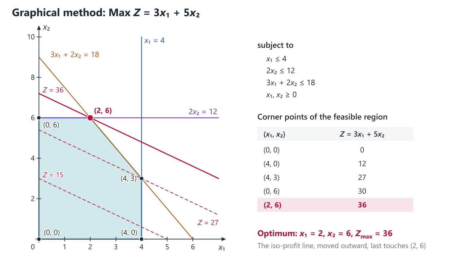
Idea: a BFS is a candidate corner that is actually feasible, i.e. a vertex of the feasible region (Theorem 2 below). In the figure above every corner of the shaded region, such as (2, 6), is a BFS, while intersections of boundary lines outside it, such as (4, 6) or (6, 0), are basic solutions that are not feasible.
Degenerate BFS: at least one basic variable is zero; a non-degenerate BFS has all m basic variables positive.
Idea: degeneracy means more constraint boundaries than necessary pass through one corner (in two variables, three or more lines through one vertex). Several different bases then describe the same point, and the simplex method may change basis without moving.
Optimal solution: a feasible solution giving the best (maximum or minimum) value of Z.
5. Fundamental Theorems
Theorem 1: The feasible region of an LPP is a convex set (an intersection of finitely many closed half-spaces and hyperplanes).
Why it works: if Ax1 = b, Ax2 = b, x1, x2 ≥ 0 and 0 ≤ λ ≤ 1, then A(λx1 + (1 − λ)x2) = λb + (1 − λ)b = b and λx1 + (1 − λ)x2 ≥ 0. So the segment joining two feasible points is feasible.
Theorem 2: A feasible x is an extreme point of the feasible region if and only if it is a basic feasible solution.
Why it works (BFS ⇒ extreme): suppose a BFS x = λu + (1 − λ)v with u, v feasible and 0 < λ < 1. Wherever xj = 0, non-negativity forces uj = vj = 0, so u and v solve the same system BxB = b, whose solution is unique; hence u = v = x.
(extreme ⇒ BFS): if the columns aj of the positive components of an extreme point x were dependent, ∑djaj = 0 with d ≠ 0 supported on those components, then x + εd and x − εd would both be feasible for small ε > 0 and x would be their midpoint, a contradiction. So those columns are independent and can be extended to a basis.
Theorem 3: If a feasible solution exists, a basic feasible solution exists.
Idea: start from any feasible x; if the columns of its positive components are dependent, move along the dependence direction d until the first component reaches 0. This keeps feasibility and reduces the number of positive components; repeating gives a BFS.
Theorem 4 (fundamental theorem): If the LPP has a finite optimal value, it is attained at at least one basic feasible solution (extreme point).
If the optimum is attained at two extreme points, it is attained at every convex combination of them (infinitely many optimal solutions).
Why it works: when the feasible region is bounded, every feasible x is a convex combination x = ∑λkxk (λk ≥ 0, ∑λk = 1) of extreme points xk. Then Z(x) = ∑λkZ(xk) ≤ maxk Z(xk), so the maximum occurs at an extreme point. If Z(x1) = Z(x2) = Z*, then Z(λx1 + (1 − λ)x2) = λZ* + (1 − λ)Z* = Z*. For an unbounded region the theorem still holds; its proof also uses the directions of unboundedness.
Idea: a linear function has no interior maximum (its gradient c never vanishes unless c = 0), so the optimum is pushed to the boundary, and along a flat face it can only improve towards a corner. This is why only finitely many points, the BFS, need be examined.
6. Understanding the Graphical Method
Why we need it: with two decision variables the whole problem can be seen in a plane: the region of allowed points and the direction in which the objective improves. This makes the corner-point principle visible and gives the answer directly.
In words: each inequality a1x + a2y ≤ b is a half-plane bounded by the line a1x + a2y = b; the feasible region is the common part of all half-planes in the first quadrant, a convex polygon (possibly unbounded). The iso-profit lines Z = k are parallel, and Z increases in the direction of the vector (c1, c2).
First example, slowly: Max Z = x + 3y subject to x + y ≤ 6, −x + y ≤ 2, x, y ≥ 0.
(1) Draw the lines: x + y = 6 through (6, 0) and (0, 6); −x + y = 2 through (0, 2) and (−2, 0).
(2) Choose the sides: the origin satisfies 0 ≤ 6 and 0 ≤ 2, so both feasible half-planes contain the origin.
(3) List the corners: (0, 0), (6, 0), (0, 2), and the meeting point of the two lines: adding them gives 2y = 8, so y = 4, x = 2.
(4) Evaluate Z: 0, 6, 6 and 2 + 12 = 14.
(5) The maximum is 14 at (2, 4). The iso-profit line x + 3y = 14 touches the region only there, because its slope −1/3 differs from the slopes −1 and 1 of the two edges at that corner, so the optimum is unique.
Non-example: the point (0, 6), where x + y = 6 meets the y-axis, looks like a corner on the sketch of the first line alone, but it violates −x + y ≤ 2 (6 > 2). It is a basic solution that is not feasible, and its value Z = 18 must not be used.
Building up: (i) A linear function on a convex polygon is largest at a vertex, because every point is a weighted average of vertices (fundamental theorem). (ii) If the objective line is parallel to the optimal edge, every point of that edge is optimal. (iii) On an unbounded region, decide boundedness of Z by looking at the directions in which the region extends.
Where it is used: every two-variable question, solving a two-variable dual graphically, and as the picture behind the simplex method.
7. Graphical Method (two variables)
Step 1: Draw each constraint as a line and identify the half-plane satisfying the inequality.
Step 2: Mark the feasible region: the common region in the first quadrant.
Step 3: Find every corner point by solving pairs of boundary lines and checking the remaining constraints.
Step 4: Evaluate Z at each corner and pick the best; equivalently move the iso-profit line Z = k in the improving direction until it last touches the region.
Why the iso-profit line works: the lines Z = k are parallel, and Z increases in the direction of the vector (c1, c2). Sliding the line in that direction, the last contact with the region is a corner or a whole edge: the fundamental theorem in a picture. In the figure above Z = 3x1 + 5x2 last touches the region at (2, 6), giving Z = 36.
Special cases: empty region (infeasible); unbounded region with Z improving without limit (unbounded solution); iso-profit line parallel to a binding edge (alternative optima); a redundant constraint that does not affect the region.
Diagnosing alternative optima: they occur when the objective line is parallel to a binding constraint at the optimum, i.e. c1/c2 = a1/a2 for that constraint a1x1 + a2x2 ≤ b, and that edge is the last contact. An unbounded region does not by itself mean an unbounded solution; it depends on the direction of improvement.
Example 1: Max Z = 3x + 2y subject to x + y ≤ 4, x + 3y ≤ 6, x, y ≥ 0.
Corners: (0, 0), (4, 0), (3, 1) from x + y = 4 and x + 3y = 6, and (0, 2); Z = 0, 12, 11, 4.
Maximum Z = 12 at x = 4, y = 0.
Example 2: Find all basic solutions of x1 + 2x2 + x3 = 4, 2x1 + x2 + 5x3 = 5.
Basis (x1, x2): x1 = 2, x2 = 1, x3 = 0; basic feasible and non-degenerate.
Basis (x1, x3): x1 = 5, x3 = −1, x2 = 0; basic but not feasible.
Basis (x2, x3): x2 = 5/3, x3 = 2/3, x1 = 0; basic feasible and non-degenerate.
8. Choosing the Method
If there are two decision variables → the graphical method, however many constraints there are.
If there are three or more variables, all constraints ≤ and b ≥ 0 → the simplex method with slack variables as the starting basis.
If some constraints are ≥ or = → Big-M or two-phase method (next topic); if there are many constraints but only two variables in the dual → solve the dual graphically.
If asked to find all basic solutions → list the C(n, m) choices of m columns, solve each m × m system, discard singular choices, and classify each solution as feasible or not, degenerate or not.
If asked to show that a given point is (or is not) a BFS or an extreme point → check feasibility, then check that the columns of its positive components are linearly independent.
If the problem has a supply–demand or one-to-one matching structure → use the transportation or assignment algorithm rather than the general simplex method.
9. Common Mistakes
1. Not defining the decision variables with units, or omitting the non-negativity conditions, in a formulation question.
2. Shading the wrong side of a constraint line; test a point such as the origin in each inequality.
3. Evaluating Z at intersection points that violate another constraint, such as (4, 6) in the figure above.
4. Declaring an unbounded solution just because the region is unbounded; a minimisation with positive costs over such a region usually has a finite optimum.
5. Counting basic solutions as C(n, m) without removing singular choices, or forgetting that a degenerate basic solution is still basic.
6. Reporting a single optimum when the objective is parallel to the optimal edge; state that every point of the edge is optimal and give the edge.
Link: basic solutions are solutions of m × m linear systems BxB = b, so rank, linear independence and Cramer's rule from Linear Algebra decide which column choices work.
Link: Lagrange multipliers (Calculus) handle smooth objectives with equality constraints at interior critical points; a linear objective has no critical points, so LP optima lie on the boundary, and the dual variables of the duality topic play the role of the multipliers.
10. Worked Examples
Example 3: A firm makes chairs (x) and tables (y) with profits Rs 40 and Rs 30 per unit. A chair needs 2 h of machining and 1 h of finishing, a table 1 h of each; 100 machining hours and 80 finishing hours are available, and at most 40 chairs can be sold. Formulate and solve graphically.
Max Z = 40x + 30y subject to 2x + y ≤ 100, x + y ≤ 80, x ≤ 40, x, y ≥ 0.
Corners: (0, 0), (40, 0), (40, 20) from x = 40 and 2x + y = 100, (20, 60) from 2x + y = 100 and x + y = 80, and (0, 80).
Z = 0, 1600, 2200, 2600, 2400, so Max Z = 2600 at x = 20, y = 60; the constraint x ≤ 40 is not binding at the optimum.
Example 4: Min Z = 3x + 2y subject to x + y ≥ 4, x + 3y ≥ 6, x, y ≥ 0.
The feasible region lies above both lines and is unbounded, but Z ≥ 0 on it, so a minimum exists and is attained at a corner.
Corners: (0, 4), (3, 1) from x + y = 4 and x + 3y = 6, and (6, 0); Z = 8, 11, 18, so Min Z = 8 at x = 0, y = 4.
Example 5: Show that Max Z = 2x + 3y subject to x − y ≤ 2, x + y ≥ 4, x, y ≥ 0 has an unbounded solution.
For every t ≥ 4 the point (0, t) is feasible, since x − y = −t ≤ 2 and x + y = t ≥ 4; on these points Z = 3t → ∞, so there is no finite maximum.
Min Z on the same region is finite: the only corners are (0, 4) and (3, 1), with Z = 12 and 9, so Min Z = 9 at (3, 1).
Example 6: Max Z = 2x + 4y subject to x + 2y ≤ 5, x + y ≤ 4, x, y ≥ 0. Show that there are infinitely many optimal solutions.
Corners: (0, 0), (4, 0), (3, 1) and (0, 5/2), with Z = 0, 8, 10, 10; the maximum 10 occurs at two adjacent corners because the line 2x + 4y = k is parallel to the edge x + 2y = 5.
Every point λ(3, 1) + (1 − λ)(0, 5/2) = (3λ, 5/2 − 3λ/2), 0 ≤ λ ≤ 1, is optimal, since Z = 6λ + 10 − 6λ = 10.
Example 7: x1 = x2 = x3 = 1 is a feasible solution of x1 + 2x2 + x3 = 4, 2x1 + x2 + 5x3 = 8. Reduce it to a basic feasible solution.
The columns a1 = (1, 2), a2 = (2, 1), a3 = (1, 5) are dependent: a3 = 3a1 − a2, so 3a1 − a2 − a3 = 0 with λ = (3, −1, −1).
Only λ1 > 0, so θ = min{xj/λj : λj > 0} = 1/3, and xj − θλj gives (1 − 1, 1 + 1/3, 1 + 1/3) = (0, 4/3, 4/3).
Check: 8/3 + 4/3 = 4 and 4/3 + 20/3 = 8; a2, a3 are independent (det [[2, 1], [1, 5]] = 9 ≠ 0), so (0, 4/3, 4/3) is a non-degenerate BFS.
11. Counting Basic Solutions, Degeneracy and Existence of an Optimum
Singular choices: m chosen columns give a basic solution only if they are linearly independent. If two chosen columns are proportional (determinant 0), that choice gives no basic solution (the reduced system is then inconsistent or has infinitely many solutions). So the number of basic solutions is C(n, m) minus the number of singular choices.
Classifying each basic solution: feasible if every basic variable is ≥ 0; degenerate if some basic variable is 0; non-degenerate if all m basic variables are non-zero (positive, for a BFS). Report the count of each type when asked.
Existence of an optimum without solving: if the feasible region is non-empty and bounded (for example, every variable is bounded by an equation with non-negative coefficients), the linear objective attains its maximum and minimum on this closed bounded set, so a finite optimum exists and is attained at a BFS. Evaluate Z at all BFS; a tie between two BFS gives alternative optima on the whole segment joining them.
Unbounded region: an optimum may still exist (for instance a Min problem with positive costs, where Z ≥ 0), but this must be argued, not assumed.
12. Formulation Patterns: Mixtures, Requirements and Cutting Stock
Mixtures: if mixture j combines resources in the ratio p : q : r, one ton of it contains p/(p + q + r) ton of the first resource, and so on; the stock of each resource gives a ≤ constraint.
Requirements (diet type): minimum requirements give ≥ constraints; the region is unbounded, but with positive costs the minimum exists at a corner.
Cutting stock (trim loss): list every cutting pattern of the stock length (how many pieces of each required length it yields), keeping only patterns whose leftover is shorter than the shortest required piece. Let xj be the number of stock pieces cut by pattern j; each required length gives one constraint, and the objective is Min ∑(trim of pattern j)xj.
With the requirements written as equations, total trim = (stock length)×(pieces used) − (total length required), so minimising trim is the same as minimising the number of stock pieces used.
13. Past UPSC Questions Solved
Example 8 (UPSC 2015, 20 marks): Consider the following linear programming problem:
Maximize Z = x1 + 2x2 − 3x3 + 4x4
subject to
x1 + x2 + 2x3 + 3x4 = 12
x2 + 2x3 + x4 = 8
x1, x2, x3, x4 ≥ 0
(i) Using the definition, find its all basic solutions. Which of these are degenerate basic feasible solutions and which are non-degenerate basic feasible solutions?
(ii) Without solving the problem, show that it has an optimal solution. Which of the basic feasible solution(s) is/are optimal?
(i) n = 4, m = 2, so at most C(4, 2) = 6 bases. The columns are a1 = (1, 0), a2 = (1, 1), a3 = (2, 2), a4 = (3, 1); a3 = 2a2, so (x2, x3) is singular (it gives x2 + 2x3 = 12 and x2 + 2x3 = 8, which are inconsistent).
(x1, x2): x2 = 8, x1 = 4, giving (4, 8, 0, 0), a BFS with Z = 20. (x1, x3): 2x3 = 8, x1 = 4, giving (4, 0, 4, 0), a BFS with Z = −8.
(x1, x4): x4 = 8, x1 = 12 − 24 = −12, basic but not feasible. (x2, x4): x2 + 3x4 = 12, x2 + x4 = 8 give (0, 6, 0, 2), a BFS with Z = 20. (x3, x4): 2x3 + 3x4 = 12, 2x3 + x4 = 8 give (0, 0, 3, 2), a BFS with Z = −1.
So there are 5 basic solutions; 4 are basic feasible, and all 4 are non-degenerate (every basic variable is positive). There is no degenerate BFS.
(ii) The second equation with x ≥ 0 gives x2, x4 ≤ 8 and x3 ≤ 4, and the first gives x1 ≤ 12. So the feasible set is non-empty, closed and bounded, and the linear Z attains a finite maximum, at a BFS (fundamental theorem).
Comparing Z at the four BFS, the maximum 20 is attained at (4, 8, 0, 0) and (0, 6, 0, 2), hence at every λ(4, 8, 0, 0) + (1 − λ)(0, 6, 0, 2), 0 ≤ λ ≤ 1.
Answer: 5 basic solutions, 4 of them non-degenerate BFS and none degenerate; the optimal BFS are (4, 8, 0, 0) and (0, 6, 0, 2), with Max Z = 20.
Example 9 (UPSC 2018, 15 marks): How many basic solutions are there in the following linearly independent set of equations ? Find all of them.
2x1 − x2 + 3x3 + x4 = 6
4x1 − 2x2 − x3 + 2x4 = 10.
Here m = 2 and n = 4, so there are at most C(4, 2) = 6 basic solutions. The columns are a1 = (2, 4), a2 = (−1, −2), a3 = (3, −1), a4 = (1, 2).
a1, a2, a4 are all multiples of (1, 2), so the pairs (x1, x2), (x1, x4), (x2, x4) are singular. With x3 = 0 the equations read 2x1 − x2 + x4 = 6 and 2(2x1 − x2 + x4) = 10, which are inconsistent, so these give no solution.
(x1, x3): 2x1 + 3x3 = 6, 4x1 − x3 = 10 give x1 = 18/7, x3 = 2/7.
(x2, x3): −x2 + 3x3 = 6, −2x2 − x3 = 10 give x2 = −36/7, x3 = 2/7.
(x3, x4): 3x3 + x4 = 6, −x3 + 2x4 = 10 give x3 = 2/7, x4 = 36/7.
Answer: exactly 3 basic solutions: (18/7, 0, 2/7, 0), (0, −36/7, 2/7, 0) and (0, 0, 2/7, 36/7).
Example 10 (UPSC 2025, 10 marks): How many basic solutions are there for the following system of equations?
2x1 − x2 + 3x3 + x4 = 6
4x1 − 2x2 − x3 + 2x4 = 10
Find all of them. Furthermore, find the number of basic solutions, which are feasible/non-feasible/non-degenerate.
This is the system of Example 9: 3 of the 6 column pairs are singular, so there are 3 basic solutions.
(18/7, 0, 2/7, 0) and (0, 0, 2/7, 36/7) have both basic variables positive, so they are basic feasible and non-degenerate.
(0, −36/7, 2/7, 0) has x2 < 0, so it is basic but not feasible; it is also non-degenerate, since no basic variable is 0.
Answer: 3 basic solutions: 2 feasible, 1 non-feasible, and all 3 non-degenerate (none is degenerate).
Example 11 (UPSC 2020, 10 marks): UPSC maintenance section has purchased sufficient number of curtain cloth pieces to meet the curtain requirement of its building. The length of each piece is 17 feet. The requirement according to curtain length is as follows :
Curtain length (in feet) : 5, 9, 7
Number required : 700, 400, 300
The width of all curtains is same as that of available pieces. Form a linear programming problem in standard form that decides the number of pieces cut in different ways so that the total trim loss is minimum. Also give a basic feasible solution to it.
Patterns for a 17 ft piece (pieces of 5, 9, 7 ft; leftover under 5 ft): P1 = (3, 0, 0), trim 2; P2 = (2, 0, 1), trim 0; P3 = (1, 1, 0), trim 3; P4 = (0, 1, 1), trim 1; P5 = (0, 0, 2), trim 3.
Let xj be the number of pieces cut by pattern Pj. Minimise Z = 2x1 + 0x2 + 3x3 + x4 + 3x5.
Subject to 3x1 + 2x2 + x3 = 700 (5 ft), x3 + x4 = 400 (9 ft), x2 + x4 + 2x5 = 300 (7 ft), xj ≥ 0 (integers). Equations stop surplus curtains being counted as useful, and this is the standard form (equality constraints, b ≥ 0, x ≥ 0).
A BFS: take the basis (x1, x3, x5) with x2 = x4 = 0. Then x3 = 400, 3x1 = 300 so x1 = 100, and 2x5 = 300 so x5 = 150; the columns (3, 0, 0), (1, 1, 0), (0, 0, 2) are independent and all values are ≥ 0.
This BFS has trim 200 + 1200 + 450 = 1850 ft. (Checking all bases, the minimum trim is 1000 ft, for example x1 = 200, x3 = 100, x4 = 300, using 600 pieces.)
Answer: Min Z = 2x1 + 3x3 + x4 + 3x5 subject to the three equations above, x ≥ 0; a BFS is (x1, ..., x5) = (100, 0, 400, 0, 150).
14. Practice Exercises
Exercise 1 (basic): Write in standard form: Min Z = 2x1 − x2 subject to x1 + x2 ≥ 2, x1 − x2 ≤ 3, x1 ≥ 0, x2 unrestricted.
Answer: with x2 = x2′ − x2″: Max Z′ = −2x1 + x2′ − x2″ subject to x1 + x2′ − x2″ − s1 = 2, x1 − x2′ + x2″ + s2 = 3, all variables ≥ 0.
Exercise 2 (basic): Is (1, 1, 1) a basic solution of x1 + x2 + x3 = 3, x1 − x2 = 0?
Answer: no: it is feasible, but it has three non-zero components while m = 2, so it cannot be basic (the three columns are dependent).
Exercise 3 (basic): At most how many basic solutions can a system of 3 independent equations in 5 unknowns have?
Answer: C(5, 3) = 10.
Exercise 4 (standard): Solve graphically: Max Z = 4x + 5y subject to x + y ≤ 5, x + 3y ≤ 9, x ≤ 4, x, y ≥ 0.
Answer: corners (0, 0), (4, 0), (4, 1), (3, 2), (0, 3) with Z = 0, 16, 21, 22, 15: Max Z = 22 at (3, 2).
Exercise 5 (standard): Solve graphically: Min Z = 5x + 2y subject to 3x + y ≥ 6, x + y ≥ 4, x + 3y ≥ 6, x, y ≥ 0.
Answer: corners (0, 6), (1, 3), (3, 1), (6, 0) with Z = 12, 11, 17, 30: Min Z = 11 at (1, 3); the region is unbounded but Z ≥ 0 on it.
Exercise 6 (standard): Find all basic solutions of x1 + x2 + 2x3 = 4, 2x1 − x2 + x3 = 2 and classify them.
Answer: (x1, x2): (2, 2, 0), a non-degenerate BFS; (x1, x3) and (x2, x3) both give (0, 0, 2), a degenerate BFS (one basic variable is 0), the same point from two bases.
Exercise 7 (standard): Show that Max Z = 3x + 6y subject to x + 2y ≤ 8, x + y ≤ 6, x, y ≥ 0 has infinitely many optimal solutions, and describe them.
Answer: corners (0, 0), (6, 0), (4, 2), (0, 4) give Z = 0, 18, 24, 24; every point λ(4, 2) + (1 − λ)(0, 4), 0 ≤ λ ≤ 1, is optimal with Z = 24 (Z is parallel to x + 2y = 8).
Exercise 8 (UPSC level): (2, 1, 1) is a feasible solution of x1 + x2 + x3 = 4, 2x1 + x2 + 3x3 = 8. Reduce it to a basic feasible solution.
Answer: a3 = 2a1 − a2, so d = (2, −1, −1); θ = 2/2 = 1 gives (0, 2, 2), a non-degenerate BFS (using −d instead gives the degenerate BFS (4, 0, 0)).
Exercise 9 (UPSC level): A farmer has 100 acres. Wheat gives a profit of Rs 4000 per acre and needs 3 man-days per acre; rice gives Rs 5000 per acre and needs 5 man-days per acre. 400 man-days are available and at most 60 acres may be under rice. Formulate and solve.
Answer: Max Z = 4000x + 5000y, x + y ≤ 100, 3x + 5y ≤ 400, y ≤ 60, x, y ≥ 0; corners (0, 0), (100, 0), (50, 50), (100/3, 60), (0, 60): Max Z = Rs 4,50,000 with 50 acres of each.
Exercise 10 (UPSC level): Find all basic solutions of 2x1 + 3x2 − x3 + 4x4 = 8, x1 − 2x2 + 6x3 − 7x4 = −3, and the BFS that maximises Z = 2x1 + 3x2 + 4x3 + 7x4.
Answer: six bases; BFS (1, 2, 0, 0), (22/9, 0, 0, 7/9), (0, 45/16, 7/16, 0), (0, 0, 44/17, 45/17) with Z = 8, 31/3, 163/16, 491/17; (45/13, 0, −14/13, 0) and (0, 44/13, 0, −7/13) are infeasible. Max Z = 491/17 at (0, 0, 44/17, 45/17).
| Case | Graphical method | Simplex table |
|---|---|---|
| Alternative optima | Iso-profit line parallel to a binding edge | A non-basic Δj = 0 in the optimal table |
| Unbounded solution | Region open in the improving direction | Entering column has no positive entry |
| Infeasible problem | No common feasible region | Artificial variable positive in the final basis |
| Degeneracy | Three or more constraint lines through one corner | Tie in the minimum ratio or a basic variable equal to 0 |
Mains points
- Formulation questions (product mix, diet, blending) give marks for clearly defining decision variables, the objective function and every constraint, including non-negativity.
- For 'find all basic solutions', list every one of the C(n, m) choices of basis, solve each, and classify it as feasible or infeasible and degenerate or non-degenerate.
- In graphical answers draw a neat labelled graph, shade the feasible region, tabulate corner points with their Z values and state the optimum clearly.
- Proofs that the feasible region is convex and that BFSs are exactly the extreme points are standard theory questions; state the hypotheses (rank A = m, b ≥ 0).
- Common mistake: using the intersection of two boundary lines as a corner without checking that it satisfies the other constraints.
Did you know?
- L. V. Kantorovich formulated linear programming models for production planning in 1939, and George Dantzig devised the simplex method in 1947; Kantorovich shared the 1975 Nobel Prize in Economics with T. C. Koopmans for the theory of optimum allocation of resources.
The Simplex Method
The simplex method moves from one basic feasible solution to an adjacent one with a better objective value until the optimality condition (all net evaluations Δj = Zj − Cj ≥ 0 for maximisation) holds. The entering variable has the most negative Δj; the leaving variable is fixed by the minimum ratio test. When ≥ or = constraints prevent an obvious starting basis, artificial variables are handled by the Big-M or two-phase method.
1. Understanding the Simplex Table
Why we need it: with three or more variables the feasible region cannot be drawn, and listing every basic solution grows quickly (C(10, 5) = 252 bases already for 5 constraints and 10 variables). We need an algebraic walk that visits only improving corners and knows when to stop.
In words: a simplex table lists the current basic variables, their costs cB and values xB, and for every variable its column yj (how it is expressed through the basis). The net evaluation Δj = cBTyj − cj is the amount by which Z would fall per unit of xj brought in; so a negative Δj (in a Max problem) means that bringing xj in raises Z.
First example, slowly: Max Z = 2x1 + 3x2 subject to x1 + x2 ≤ 4, x1 + 3x2 ≤ 6, x ≥ 0 (columns x1, x2, s1, s2 | xB).
(1) Table 1: s1: 1, 1, 1, 0 | 4; s2: 1, 3, 0, 1 | 6; Δj: −2, −3, 0, 0 | Z = 0. This is the corner (0, 0).
(2) The most negative Δ is −3, so x2 enters. Ratios 4/1 = 4 and 6/3 = 2: the least is in row s2, which leaves; the key element is 3.
(3) Table 2 (divide the key row by 3, then clear the column): x2: 1/3, 1, 0, 1/3 | 2; s1: 2/3, 0, 1, −1/3 | 2; Δj: −1, 0, 0, 1 | Z = 6. This is the corner (0, 2).
(4) Δ1 = 3(1/3) − 2 = −1 is negative, so x1 enters. Ratios 2/(1/3) = 6 and 2/(2/3) = 3: s1 leaves; key element 2/3.
(5) Table 3: x1: 1, 0, 3/2, −1/2 | 3; x2: 0, 1, −1/2, 1/2 | 1; Δj: 0, 0, 3/2, 1/2 | Z = 9.
(6) All Δj ≥ 0, so x1 = 3, x2 = 1, Max Z = 9. Check: the corners (0, 0), (4, 0), (3, 1), (0, 2) give 0, 8, 9, 6. Notice that the method visited (0, 0) → (0, 2) → (3, 1), adjacent corners with Z rising each time, and never looked at (4, 0).
Non-example: for a constraint x1 + x2 ≥ 4 the surplus form x1 + x2 − s1 = 4 does not give a starting BFS: putting x = 0 makes s1 = −4 < 0. The ordinary table needs an identity basis with xB ≥ 0, which fails here; artificial variables (later lesson) repair it.
Building up: (i) Every table expresses Z as Z = Z0 − ∑Δjxj over the non-basic variables (derivation section below), which proves the optimality test. (ii) The ratio test is the largest step that keeps every basic variable ≥ 0. (iii) A pivot is one Gauss–Jordan step, so the table always holds B−1A and B−1b.
Where it is used: every “solve by the simplex method” question (15–20 marks), and inside the Big-M, two-phase and dual simplex methods.
2. Simplex Algorithm (Max, all constraints ≤, b ≥ 0)
Step 1: Convert to standard form with slack variables; the slacks form the initial basis (identity matrix) and give the initial BFS.
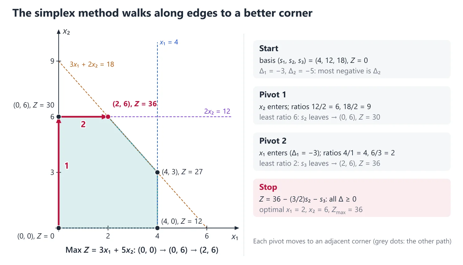
Idea: the simplex method walks along the edges of the feasible region from one corner (BFS) to an adjacent better one, and stops at a corner from which no edge improves Z. Algebraically, adjacent corners differ by one basic variable: one variable enters the basis and one leaves.
Step 2: For each non-basic column compute the net evaluation Δj = Zj − Cj = cBTyj − cj, where yj is the current column of xj.
Optimality test: if every Δj ≥ 0, the current BFS is optimal.
Step 3 (entering variable): choose the most negative Δk; xk enters (key column).
Unboundedness test: if every entry yik ≤ 0 in the key column, the problem has an unbounded solution.
Step 4 (leaving variable): for yik > 0 form the ratios xBi/yik; the row with the least ratio leaves (key row) and yrk is the key element.
Step 5 (pivoting): divide the key row by the key element and reduce every other entry of the key column to zero by row operations; return to Step 2.
Each iteration moves to an adjacent extreme point and Z does not decrease; in the absence of degeneracy Z strictly increases, so the method ends in finitely many steps.
3. Derivation: Why the Optimality and Ratio Tests Work
Split A = [B N] and x = (xB, xN). From Ax = b, xB = B−1b − ∑j∈N yjxj, where yj = B−1aj is the column of xj in the current table.
Substituting in Z = cBTxB + ∑j∈N cjxj gives Z = cBTB−1b − ∑j∈N (cBTyj − cj)xj = Z0 − ∑j∈N Δjxj, an identity valid for every feasible x.
Optimality test: if every Δj ≥ 0, then, since every xj ≥ 0, Z ≤ Z0 for every feasible x, so the current BFS (Z = Z0) is optimal.
Entering variable: if Δk < 0, raising xk from 0 to t (other non-basic variables kept at 0) gives Z = Z0 − Δkt, which increases at the rate |Δk| per unit. The most negative Δk (Dantzig's rule) gives the fastest rate per unit, not necessarily the largest total gain.
Ratio test: the basic variables become xBi = x̂Bi − t yik, where x̂Bi is the current value. A row with yik ≤ 0 never becomes negative; a row with yik > 0 stays ≥ 0 only while t ≤ x̂Bi/yik. So the largest step is t* = min{x̂Bi/yik : yik > 0}, and the basic variable of the row attaining it drops to 0 and leaves.
Unboundedness: if every yik ≤ 0, no basic variable ever becomes negative, t can grow without limit, and Z = Z0 − Δkt → ∞.
Pivoting and termination: the row operations of Step 5 compute the new B−1, so every table shows B−1A and B−1b. There are at most C(n, m) bases; when no BFS is degenerate, t* > 0 and Z strictly increases, so no basis repeats and the method stops after finitely many iterations.
4. Understanding the Signals in a Simplex Table
Why we need it: the final table answers more than “what is the optimum”. Questions ask whether the optimum is unique, whether the problem is unbounded or infeasible, and whether degeneracy occurred; each has a definite signal in the table.
In words: (a) a non-basic variable with Δj = 0 in an optimal table means another optimal corner can be reached; (b) an entering column with no positive entry means Z can grow without bound; (c) a tie in the ratio test, or a basic variable equal to 0, means degeneracy; (d) an artificial variable left positive means infeasibility.
First example, slowly: Max Z = x1 + x2 subject to x1 + x2 ≤ 4, x1 ≤ 3, x ≥ 0.
(1) Table 1: s1: 1, 1, 1, 0 | 4; s2: 1, 0, 0, 1 | 3; Δj: −1, −1, 0, 0. The tie between −1 and −1 is broken by taking x1; ratios 4 and 3, so s2 leaves.
(2) Table 2: x1: 1, 0, 0, 1 | 3; s1: 0, 1, 1, −1 | 1; Δj: 0, −1, 0, 1 | Z = 3. Now x2 enters; only row s1 has a positive entry, ratio 1, so s1 leaves.
(3) Table 3: x2: 0, 1, 1, −1 | 1; x1: 1, 0, 0, 1 | 3; Δj: 0, 0, 1, 0 | Z = 4. All Δj ≥ 0: (3, 1) is optimal.
(4) Read the signal: s2 is non-basic with Δ = 0. Bring it in: its column is (−1, 1), so only row x1 gives a ratio, 3/1 = 3, and x1 leaves.
(5) The new BFS is x1 = 0, x2 = 4, s2 = 3 with the same Z = 4. So (3, 1) and (0, 4) are both optimal, and so is every point between them. Notice the geometry: Z = x1 + x2 is parallel to the edge x1 + x2 = 4.
Non-example: a zero Δj under a basic variable is no signal at all: every basic column is a unit vector ei, so Δj = cBTei − cj = cj − cj = 0 always. Only a zero under a non-basic variable indicates alternative optima.
Building up: (i) From Z = Z0 − ∑Δjxj, a zero Δj lets xj grow without changing Z. (ii) If the entering column has no positive entry, xB = x̂B − t yk stays ≥ 0 for all t, so Z → ∞. (iii) A tie in the ratio test leaves a basic variable at 0; the next step may then have t* = 0, and the basis changes without moving.
Where it is used: the final sentence of every simplex answer, which should state uniqueness or alternative optima, and the “show that the problem is unbounded (or infeasible)” questions.
5. Reading the Final Table
Alternative optima: some non-basic Δj = 0 at optimality; bringing that xj in gives another optimal BFS.
Why it works: by Z = Z0 − ∑Δjxj, a zero Δj means that raising xj leaves Z unchanged; every point of the edge between the two optimal BFS is optimal. If the ratio test for that column gives t* = 0 (degenerate), the new basis describes the same point and there may be no second optimal point.
Degeneracy: a tie in the minimum ratio, or a basic variable at zero level; cycling is possible in theory and is prevented by Bland's rule or the lexicographic rule.
Idea: a tie in the minimum ratio makes two basic variables reach 0 together; one leaves and the other stays basic at value 0. At the next step t* may be 0, so the basis changes while the point and Z stay the same; cycling means such zero steps return to an earlier basis.
Infeasibility: an artificial variable stays in the optimal basis at a positive level.
Why: the artificial variables measure how far the original constraints are from being satisfied. If even the best table keeps one positive, there is no point at which all the original constraints hold.
Minimisation: use Min Z = −Max(−Z), or enter the most positive Δj and stop when all Δj ≤ 0.
6. Understanding Artificial Variables (Big-M and Two-Phase)
Why we need it: the simplex method must start at a BFS with an identity basis. Constraints of type ≥ or = do not supply one, so we add temporary variables that give a start, and then force them out.
In words: an artificial variable ai ≥ 0 is added to a ≥ or = row so that its column is a unit vector. A point with some ai > 0 is not a solution of the original problem. Big-M makes such points very expensive (cost −M in a Max problem); the two-phase method first minimises ∑ai alone (Phase I) and only then the real objective (Phase II).
First example, slowly: Phase I for the constraints x1 + 2x2 ≥ 4, x1 + x2 ≤ 3, x ≥ 0.
(1) Write the rows: x1 + 2x2 − s1 + a1 = 4 and x1 + x2 + s2 = 3. The starting basis is (a1, s2) = (4, 3), an identity basis with non-negative values.
(2) Phase I objective: Max Z* = −a1, so cB = (−1, 0). The net evaluations (columns x1, x2, s1, s2, a1) are −1, −2, 1, 0, 0, and Z* = −4.
(3) x2 enters (most negative); ratios 4/2 = 2 and 3/1 = 3, so a1 leaves.
(4) New table (artificial column dropped): x2: 1/2, 1, −1/2, 0 | 2; s2: 1/2, 0, 1/2, 1 | 1; now Z* = 0.
(5) Phase I has reached ∑ai = 0, so x = (0, 2) is a BFS of the original constraints (check: 0 + 4 = 4 ≥ 4 and 2 ≤ 3). Phase II starts from this table with the real costs. Notice that Phase I ignores the real objective completely; its only job is to find a feasible corner.
Non-example: replace the first constraint by x1 + 2x2 ≥ 8. On x1 + x2 ≤ 3 the largest value of x1 + 2x2 is 6, at (0, 3), so a1 can never drop below 2: Phase I ends with a positive artificial variable and the problem is infeasible. The condition that fails is “Phase I minimum = 0”.
Building up: (i) In Big-M every Δj has the form αM + β; since M dominates, compare α first. (ii) Phase I is an ordinary LP with a feasible start, so it always ends; its optimum is 0 exactly when the original constraints are consistent. (iii) An artificial variable basic at level 0 after Phase I is pivoted out, or its row is redundant.
Where it is used: “solve by the Big-M method” and “solve by the two-phase method” questions, Min problems with ≥ constraints, and infeasibility proofs.
7. Artificial Variables
For each ≥ or = constraint add an artificial variable ai ≥ 0 so that an identity starting basis is available.
Idea: a ≥ constraint with surplus, aix − si = bi, gives the column −ei, and si = −bi would be negative; an = constraint has no slack at all. The artificial variable is a temporary device to obtain an identity basis; it has no physical meaning and must be driven to zero.
Big-M method: give each artificial variable cost −M in a Max problem (+M in a Min problem), M very large, and apply the simplex method.
Why it works: M is so large that any solution with a positive artificial variable is worse than every solution of the original problem, so the simplex method removes the artificials first if it can. In the table each Δj has the form αM + β; compare the M-coefficients α first, and use β only to break ties.
Two-phase method: Phase I minimises the sum of artificial variables; if this minimum is 0 a BFS of the original problem is found, otherwise the problem is infeasible.
Phase II optimises the original objective starting from the final Phase I table, with the artificial columns removed.
Phase I subtlety: if the Phase I minimum is 0 but an artificial variable is still basic at value 0, pivot it out on any non-zero entry of its row under a non-artificial column; if no such entry exists, that original constraint is redundant and its row can be deleted. The two-phase method avoids the round-off problems of a numerical value for M.
8. Choosing the Method
If it is a Max problem with all constraints ≤ and b ≥ 0 → ordinary simplex with the slack basis.
If there are ≥ or = constraints → Big-M when the question names it, otherwise either; prefer two-phase when the M-arithmetic would be heavy.
If it is a Min problem → maximise −Z, or keep Min and use the reversed rules (enter the most positive Δj, stop when all Δj ≤ 0); state the convention used.
If the starting table is optimal (all Δj ≥ 0) but some bi < 0 → dual simplex method (Duality topic), with no artificial variables.
If variables have lower bounds, upper bounds or are free → substitute first (section on bounded, free and shifted variables).
If the minimum ratio is tied → choose either row (say the smaller subscript, Bland's rule) and note that the next BFS is degenerate.
9. Common Mistakes
1. Including rows with yik = 0 or yik < 0 in the ratio test; only positive entries of the key column give ratios.
2. Mixing sign conventions: with Δj = Zj − Cj a Max table is optimal when all Δj ≥ 0; some books use Cj − Zj with the opposite test. Choose one and say so.
3. Adding slacks to a row with negative right-hand side, which gives an infeasible start; multiply the row by −1 first.
4. Declaring an optimum while an artificial variable is basic at a positive level; the correct conclusion is that the problem is infeasible.
5. Overlooking a zero Δj of a non-basic variable in the final table, and so missing alternative optima that the question expects you to state.
6. In Big-M, comparing the constant parts of the Δj before their M-coefficients.
Link: each pivot is a Gauss–Jordan elimination step (Linear Algebra, Numerical Analysis), and the columns under the starting slacks always hold the current B−1.
Link: the Δj are the reduced costs yTaj − cj with yT = cBTB−1, so the optimality test is the same as feasibility of the dual (next topic).
10. Worked Examples
Example 1: Max Z = 3x1 + 5x2 subject to x1 ≤ 4, 2x2 ≤ 12, 3x1 + 2x2 ≤ 18, x1, x2 ≥ 0.
Add slacks s1, s2, s3: initial BFS (s1, s2, s3) = (4, 12, 18), Z = 0, Δ1 = −3, Δ2 = −5.
Iteration 1: x2 enters; ratios 12/2 = 6 and 18/2 = 9, so s2 leaves; now s1 = 4, x2 = 6, s3 = 6, Z = 30.
Iteration 2: Δ1 = −3, so x1 enters; ratios 4/1 = 4 and 6/3 = 2, so s3 leaves; now s1 = 2, x2 = 6, x1 = 2.
Now Z = 36 − (3/2)s2 − s3, so Δ for s2, s3 are 3/2 and 1, both ≥ 0: optimal x1 = 2, x2 = 6, Max Z = 36.
Example 2 (Big-M set-up): Min Z = 2x1 + x2 subject to 3x1 + x2 ≥ 3, x1 + x2 ≥ 2, x ≥ 0.
Write Max Z′ = −2x1 − x2 − Ma1 − Ma2 with 3x1 + x2 − s1 + a1 = 3 and x1 + x2 − s2 + a2 = 2; the starting basis is (a1, a2).
Simplex drives both artificials out and gives x1 = 1/2, x2 = 3/2, Min Z = 5/2 (check: the corners (0, 3), (1/2, 3/2), (2, 0) give Z = 3, 5/2, 4).
Example 3: Solve by the simplex method: Max Z = 3x1 + 2x2 + 5x3 subject to x1 + 2x2 + x3 ≤ 430, 3x1 + 2x3 ≤ 460, x1 + 4x2 ≤ 420, x1, x2, x3 ≥ 0.
Add slacks s1, s2, s3; all three simplex tables are given in full in the table 'Simplex Tables: Max Z = 3x1 + 2x2 + 5x3' below (key elements in square brackets).
Table 1: Δ = (−3, −2, −5), so x3 enters; ratios 430/1 = 430 and 460/2 = 230 (row 3 has no positive entry), so s2 leaves with key element 2.
Table 2: Z = 1150 and Δ2 = −2 is the only negative value; ratios 200/2 = 100 and 420/4 = 105, so s1 leaves with key element 2.
Table 3: all Δj ≥ 0, so x1 = 0, x2 = 100, x3 = 230 and Max Z = 1350 (s3 = 20 units of the third resource are unused).
Check by the dual: the Δ values under s1, s2, s3 give y = (1, 2, 0); then y1 + 3y2 + y3 = 7 ≥ 3, 2y1 + 4y3 = 2 ≥ 2, y1 + 2y2 = 5 ≥ 5, and W = 430 + 920 = 1350 = Z.
Example 4: Solve by the Big-M method: Min Z = 4x1 + x2 subject to 3x1 + x2 = 3, 4x1 + 3x2 ≥ 6, x1 + 2x2 ≤ 4, x1, x2 ≥ 0.
Max Z′ = −4x1 − x2 − Ma1 − Ma2 with 3x1 + x2 + a1 = 3, 4x1 + 3x2 − s2 + a2 = 6, x1 + 2x2 + s3 = 4; columns x1, x2, s2, s3, a1, a2 | xB.
Table 1: a1: 3, 1, 0, 0, 1, 0 | 3; a2: 4, 3, −1, 0, 0, 1 | 6; s3: 1, 2, 0, 1, 0, 0 | 4; Δj: 4 − 7M, 1 − 4M, M, 0, 0, 0 | Z′ = −9M. x1 enters; ratios 1, 3/2, 4; a1 leaves.
Table 2: x1: 1, 1/3, 0, 0, 1/3, 0 | 1; a2: 0, 5/3, −1, 0, −4/3, 1 | 2; s3: 0, 5/3, 0, 1, −1/3, 0 | 3; Δj: 0, −(1 + 5M)/3, M, 0, (7M − 4)/3, 0 | Z′ = −4 − 2M. x2 enters; ratios 3, 6/5, 9/5; a2 leaves.
Table 3: x1: 1, 0, 1/5, 0, 3/5, −1/5 | 3/5; x2: 0, 1, −3/5, 0, −4/5, 3/5 | 6/5; s3: 0, 0, 1, 1, 1, −1 | 1; Δj: 0, 0, −1/5, 0, M − 8/5, M + 1/5 | Z′ = −18/5. s2 enters; ratios 3, −, 1; s3 leaves.
Table 4: x1: 1, 0, 0, −1/5, 2/5, 0 | 2/5; x2: 0, 1, 0, 3/5, −1/5, 0 | 9/5; s2: 0, 0, 1, 1, 1, −1 | 1; Δj: 0, 0, 0, 1/5, M − 7/5, M ≥ 0, so x1 = 2/5, x2 = 9/5, Min Z = 17/5.
Check: on the line 3x1 + x2 = 3 the other two constraints give 2/5 ≤ x1 ≤ 3/5, so the only corners are (2/5, 9/5) and (3/5, 6/5), with Z = 17/5 and 18/5.
Example 5: Solve by the two-phase method: Min Z = x1 + x2 subject to 2x1 + x2 ≥ 4, x1 + 7x2 ≥ 7, x1, x2 ≥ 0.
Phase I: Max Z* = −a1 − a2 with 2x1 + x2 − s1 + a1 = 4, x1 + 7x2 − s2 + a2 = 7; columns x1, x2, s1, s2, a1, a2 | xB.
Table 1: a1: 2, 1, −1, 0, 1, 0 | 4; a2: 1, 7, 0, −1, 0, 1 | 7; Δj: −3, −8, 1, 1, 0, 0 | Z* = −11. x2 enters; ratios 4, 1; a2 leaves.
Table 2: a1: 13/7, 0, −1, 1/7, 1, −1/7 | 3; x2: 1/7, 1, 0, −1/7, 0, 1/7 | 1; Δj: −13/7, 0, 1, −1/7, 0, 8/7 | Z* = −3. x1 enters; ratios 21/13, 7; a1 leaves.
Table 3: x1: 1, 0, −7/13, 1/13 | 21/13; x2: 0, 1, 1/13, −2/13 | 10/13 (artificial columns dropped); Z* = 0, so a BFS of the original problem has been found.
Phase II (Max −Z, costs −1, −1, 0, 0): Δj = 0, 0, 6/13, 1/13 ≥ 0, so this table is already optimal: x1 = 21/13, x2 = 10/13, Min Z = 31/13; the corners (0, 4), (21/13, 10/13), (7, 0) give Z = 4, 31/13, 7.
Example 6: Show by the simplex method that Max Z = 2x1 + x2 subject to x1 − x2 ≤ 10, 2x1 − x2 ≤ 40, x1, x2 ≥ 0 is unbounded.
Table 1 (columns x1, x2, s1, s2 | xB): s1: 1, −1, 1, 0 | 10; s2: 2, −1, 0, 1 | 40; Δj: −2, −1, 0, 0 | Z = 0. x1 enters; ratios 10, 20; s1 leaves.
Table 2: x1: 1, −1, 1, 0 | 10; s2: 0, 1, −2, 1 | 20; Δj: 0, −3, 2, 0 | Z = 20. x2 enters; the only ratio is 20; s2 leaves.
Table 3: x1: 1, 0, −1, 1 | 30; x2: 0, 1, −2, 1 | 20; Δj: 0, 0, −4, 3 | Z = 80. s1 should enter, but its column (−1, −2) has no positive entry, so no variable can leave: the solution is unbounded.
Indeed x1 = 30 + t, x2 = 20 + 2t, s1 = t, s2 = 0 is feasible for every t ≥ 0 and gives Z = 80 + 4t → ∞.
Example 7: Solve Max Z = 2x1 + 4x2 subject to x1 + 2x2 ≤ 5, x1 + x2 ≤ 4, x1, x2 ≥ 0 and detect alternative optima.
Table 1: s1: 1, 2, 1, 0 | 5; s2: 1, 1, 0, 1 | 4; Δj: −2, −4, 0, 0 | Z = 0. x2 enters; ratios 5/2, 4; s1 leaves.
Table 2: x2: 1/2, 1, 1/2, 0 | 5/2; s2: 1/2, 0, −1/2, 1 | 3/2; Δj: 0, 0, 2, 0 | Z = 10. All Δj ≥ 0: optimal x1 = 0, x2 = 5/2, Z = 10.
The non-basic x1 has Δ1 = 0, the signal of an alternative optimum; entering x1 (ratios 5 and 3, so s2 leaves) gives x1 = 3, x2 = 1, again with Z = 10.
Hence every point λ(0, 5/2) + (1 − λ)(3, 1), 0 ≤ λ ≤ 1, is optimal, in agreement with the graphical solution of the same problem.
11. Bounded, Free and Shifted Variables
Lower bounds: if xj ≥ lj, put xj = yj + lj with yj ≥ 0; substitute in every constraint (the right-hand sides change) and in Z (a constant is added), solve in y, then add lj back.
Upper bounds: xj ≤ uj can be kept as an extra ≤ row with its own slack (or handled by putting xj = uj − yj when the variable reaches its bound).
Free variables: write xj = xj′ − xj″ with both parts ≥ 0; at most one of them is basic in any BFS.
Negative right-hand side: multiply the row by −1 first (the inequality reverses), so that b ≥ 0 before slacks or artificials are added.
Equations without an obvious basis: add artificial variables (Big-M or two-phase), or, if row operations give an identity sub-matrix with non-negative right-hand side, start from that basis directly.
12. Past UPSC Questions Solved
Example 8 (UPSC 2020, 15 marks): Solve the linear programming problem using simplex method :
Minimize z = −6x1 − 2x2 − 5x3
subject to 2x1 − 3x2 + x3 ≤ 14
−4x1 + 4x2 + 10x3 ≤ 46
2x1 + 2x2 − 4x3 ≤ 37
x1 ≥ 2, x2 ≥ 1, x3 ≥ 3
Put x1 = y1 + 2, x2 = y2 + 1, x3 = y3 + 3 with yj ≥ 0. The constraints become 2y1 − 3y2 + y3 ≤ 10, −4y1 + 4y2 + 10y3 ≤ 20, 2y1 + 2y2 − 4y3 ≤ 43, and z = −6y1 − 2y2 − 5y3 − 29.
Minimising z is maximising Z′ = 6y1 + 2y2 + 5y3. Add slacks s1, s2, s3; columns y1, y2, y3, s1, s2, s3 | xB.
Table 1: s1: 2, −3, 1, 1, 0, 0 | 10; s2: −4, 4, 10, 0, 1, 0 | 20; s3: 2, 2, −4, 0, 0, 1 | 43; Δj: −6, −2, −5, 0, 0, 0 | Z′ = 0. y1 enters; ratios 5, −, 43/2; s1 leaves.
Table 2: y1: 1, −3/2, 1/2, 1/2, 0, 0 | 5; s2: 0, −2, 12, 2, 1, 0 | 40; s3: 0, 5, −5, −1, 0, 1 | 33; Δj: 0, −11, −2, 3, 0, 0 | Z′ = 30. y2 enters; the only ratio is 33/5; s3 leaves.
Table 3: y1: 1, 0, −1, 1/5, 0, 3/10 | 149/10; s2: 0, 0, 10, 8/5, 1, 2/5 | 266/5; y2: 0, 1, −1, −1/5, 0, 1/5 | 33/5; Δj: 0, 0, −13, 4/5, 0, 11/5 | Z′ = 513/5. y3 enters; the only ratio is (266/5)/10 = 133/25; s2 leaves.
Table 4: y1: 1, 0, 0, 9/25, 1/10, 17/50 | 1011/50; y3: 0, 0, 1, 4/25, 1/10, 1/25 | 133/25; y2: 0, 1, 0, −1/25, 1/10, 6/25 | 298/25; Δj: 0, 0, 0, 72/25, 13/10, 68/25 | Z′ = 4294/25. All Δj ≥ 0: optimal.
Back-substituting: x1 = 1011/50 + 2 = 1111/50, x2 = 298/25 + 1 = 323/25, x3 = 133/25 + 3 = 208/25, and z = −4294/25 − 29 = −5019/25. Check: the three original constraints hold with equality (14, 46, 37).
Answer: x1 = 1111/50 = 22.22, x2 = 323/25 = 12.92, x3 = 208/25 = 8.32, Min z = −5019/25 = −200.76.
13. Practice Exercises
Exercise 1 (basic): Write the initial simplex table for Max Z = 4x1 + 3x2 subject to 2x1 + x2 ≤ 10, x1 + x2 ≤ 8, x ≥ 0, and name the entering and leaving variables.
Answer: s1: 2, 1, 1, 0 | 10; s2: 1, 1, 0, 1 | 8; Δj: −4, −3, 0, 0. x1 enters; ratios 5 and 8, so s1 leaves (key element 2).
Exercise 2 (basic): In a Max table the non-basic xk has Δk = −2 and column entries (−1, 0, −3). What do you conclude?
Answer: xk should enter but no entry is positive, so no ratio exists: the problem has an unbounded solution.
Exercise 3 (basic): Why is Δj always 0 for a basic variable?
Answer: its column in the table is the unit vector ei of its own row, so Zj = cBTei = cj.
Exercise 4 (standard): Complete the simplex solution of Exercise 1.
Answer: Table 2: x1: 1, 1/2, 1/2, 0 | 5; s2: 0, 1/2, −1/2, 1 | 3; Δ: 0, −1, 2, 0 (Z = 20). Table 3: x2 = 6, x1 = 2, Δ for s1, s2 = 1, 2: Max Z = 26.
Exercise 5 (standard): Solve by the simplex method: Max Z = 3x1 + 2x2 + 4x3 subject to x1 + x2 + 2x3 ≤ 4, 2x1 + x3 ≤ 5, 2x1 + x2 + 3x3 ≤ 7, x ≥ 0.
Answer: x1 = 5/2, x2 = 3/2, x3 = 0, Max Z = 21/2 (the first two constraints are binding; the third has slack 1/2).
Exercise 6 (standard): Solve by the Big-M method: Min Z = 2x1 + 3x2 subject to x1 + x2 ≥ 5, x1 + 3x2 ≥ 9, x ≥ 0.
Answer: x1 = 3, x2 = 2, Min Z = 12 (check: the corners (0, 5), (3, 2), (9, 0) give 15, 12, 18).
Exercise 7 (standard): Use Phase I to show that x1 + x2 ≤ 1, 2x1 + 3x2 ≥ 6, x ≥ 0 has no feasible solution.
Answer: x2 enters and s1 leaves; the next table has all Δ ≥ 0 with a1 = 3 > 0, so the system is infeasible (indeed 2x1 + 3x2 ≤ 3 on the first constraint).
Exercise 8 (UPSC level): Solve by the Big-M method: Max Z = 3x1 − x2 subject to 2x1 + x2 ≥ 2, x1 + 3x2 ≤ 3, x2 ≤ 4, x ≥ 0.
Answer: x1 = 3, x2 = 0, Max Z = 9 (the feasible corners are (1, 0), (3, 0), (3/5, 4/5) with Z = 3, 9, 1; the constraint x2 ≤ 4 is redundant).
Exercise 9 (UPSC level): Apply the two-phase method to Min Z = x1 − 2x2 − 3x3 subject to −2x1 + x2 + 3x3 = 2, 2x1 + 3x2 + 4x3 = 1, x ≥ 0.
Answer: Phase I ends with a1 + a2 = 5/4 > 0 (at x3 = 1/4), so the problem is infeasible. Directly: x1 ≥ 0 needs x2 + 3x3 ≥ 2, and then the second equation forces x2 < 0.
Exercise 10 (UPSC level): Solve Max Z = 2x1 + x2 subject to x1 + x2 ≤ 10, x1 ≤ 6, x1 ≥ 2, x2 ≥ 1, by first shifting the variables.
Answer: x1 = y1 + 2, x2 = y2 + 1 give y1 + y2 ≤ 7, y1 ≤ 4, Z = 2y1 + y2 + 5; the simplex method gives y = (4, 3), so x = (6, 4) and Max Z = 16.
| Feature | Big-M method | Two-phase method |
|---|---|---|
| Cost of artificial variable | −M (Max) or +M (Min) | 1 in Phase I objective, 0 for others |
| Number of stages | One | Two (Phase I feasibility, Phase II optimality) |
| Sign of infeasibility | Artificial positive in the optimal basis | Phase I minimum > 0 |
| Practical note | Large M causes round-off error on computers | Avoids M; preferred in computer codes |
| Table | Basis | cB | xB | x1 | x2 | x3 | s1 | s2 | s3 | Ratio |
|---|---|---|---|---|---|---|---|---|---|---|
| 1 | s1 | 0 | 430 | 1 | 2 | 1 | 1 | 0 | 0 | 430 |
| 1 | s2 | 0 | 460 | 3 | 0 | [2] | 0 | 1 | 0 | 230 (least) |
| 1 | s3 | 0 | 420 | 1 | 4 | 0 | 0 | 0 | 1 | − |
| 1 | Δj | Z = 0 | −3 | −2 | −5 | 0 | 0 | 0 | x3 enters, s2 leaves | |
| 2 | s1 | 0 | 200 | −1/2 | [2] | 0 | 1 | −1/2 | 0 | 100 (least) |
| 2 | x3 | 5 | 230 | 3/2 | 0 | 1 | 0 | 1/2 | 0 | − |
| 2 | s3 | 0 | 420 | 1 | 4 | 0 | 0 | 0 | 1 | 105 |
| 2 | Δj | Z = 1150 | 9/2 | −2 | 0 | 0 | 5/2 | 0 | x2 enters, s1 leaves | |
| 3 | x2 | 2 | 100 | −1/4 | 1 | 0 | 1/2 | −1/4 | 0 | |
| 3 | x3 | 5 | 230 | 3/2 | 0 | 1 | 0 | 1/2 | 0 | |
| 3 | s3 | 0 | 20 | 2 | 0 | 0 | −2 | 1 | 1 | |
| 3 | Δj | Z = 1350 | 4 | 0 | 0 | 1 | 2 | 0 | Optimal |
Mains points
- A full simplex problem (often 15–20 marks) is expected: show every table with cB, basis, xB, the Δj row, ratios, and mark the key element.
- State the entering and leaving variables with the reason (most negative Δj, least ratio) at each iteration; examiners award step marks for this.
- Questions often ask for the problem by Big-M or two-phase specifically; using the other method may lose marks.
- End with an explicit conclusion: optimal values of all decision variables and Z, and note alternative optima or unboundedness if the table shows it.
- Common mistakes: forgetting to convert Min to Max consistently, arithmetic slips in pivoting, and leaving an artificial variable in the basis without comment.
Did you know?
- The simplex method takes exponentially many steps on the Klee–Minty cube (1972), yet it is fast in practice; Khachiyan (1979) and Karmarkar (1984) later gave polynomial-time algorithms for LP.
Duality in Linear Programming
Every LPP (the primal) has a partner LPP (the dual) built from the same data: constraints and variables swap roles, the cost vector and right-hand side interchange, and A is transposed. The weak duality theorem bounds one objective by the other, the strong duality theorem says the optimal values are equal, and complementary slackness links optimal primal and dual solutions. Optimal dual values are the shadow prices of resources and can be read from the final simplex table.
1. Understanding the Dual Problem
Why we need it: a Max problem gives lower bounds (any feasible point has a value below the optimum), but how do we know that a proposed answer cannot be beaten? The dual is a second LP, built from the same numbers, whose feasible points give upper bounds. It also prices the resources and is sometimes much easier to solve.
In words: attach one dual variable yi to each primal constraint and write one dual constraint for each primal variable. The right-hand sides b become the dual costs, the costs c become the dual right-hand sides, the matrix is transposed, and Max becomes Min. For the canonical form (Max, all ≤, x ≥ 0) every dual variable is ≥ 0 and every dual constraint is ≥.
First example, slowly: Max Z = 3x1 + 2x2 subject to x1 + x2 ≤ 4, x1 + 3x2 ≤ 6, x ≥ 0.
(1) Attach y1 ≥ 0 to the first constraint and y2 ≥ 0 to the second (both are ≤ rows of a Max problem).
(2) Dual objective: the right-hand sides 4 and 6 become costs, Min W = 4y1 + 6y2.
(3) Column of x1 is (1, 1) with cost 3: y1 + y2 ≥ 3. Column of x2 is (1, 3) with cost 2: y1 + 3y2 ≥ 2.
(4) The primal optimum is Z = 12 at (4, 0). Try y = (3, 0): 3 ≥ 3 and 3 ≥ 2, so y is dual feasible, and W = 12.
(5) Equal values for a feasible pair prove that both are optimal (weak duality, next lesson). Notice the meaning of y1 = 3: one more unit of the first resource would add 3 to the maximum profit, while the second resource is not scarce (y2 = 0).
Non-example: Max Z = x1 + x2 subject to x1 + 2x2 ≥ 2, x ≥ 0 is unbounded. Writing its dual carelessly with y ≥ 0 gives Min 2y, y ≥ 1, 2y ≥ 1, which has the finite optimum 2, impossible for the dual of an unbounded problem. The ≥ row of a Max problem needs y ≤ 0; then y ≥ 1 cannot hold and the dual is infeasible, as it must be.
Building up: (i) Multiplying each constraint by yi ≥ 0 and adding gives yTAx ≤ yTb; if ATy ≥ c this bounds cTx, and the dual asks for the smallest such bound (derivation section below). (ii) The sign rules for = and ≥ rows and for free variables follow from the same multiplication argument. (iii) The dual of the dual is the primal.
Where it is used: “write the dual” questions, solving a two-variable dual graphically, reading shadow prices, and the u, v of the transportation MODI method.
2. Formulating the Dual
Symmetric pair: Primal: Max Z = cTx subject to Ax ≤ b, x ≥ 0. Dual: Min W = bTy subject to ATy ≥ c, y ≥ 0.
Idea (economic): the primal is a producer choosing outputs x to maximise profit from limited resources b. The dual is a buyer who offers a price yi per unit of resource i, high enough that each product's resources are worth at least its profit (ATy ≥ c), and who wants to pay as little as possible for all the resources (Min bTy).
Each primal constraint gives one dual variable and each primal variable gives one dual constraint; c and b interchange; A becomes AT.
Rules (primal Max): constraint ≤ gives dual variable ≥ 0; constraint = gives dual variable unrestricted in sign; constraint ≥ gives dual variable ≤ 0.
Primal variable xj ≥ 0 gives dual constraint ≥; xj unrestricted gives dual constraint =.
To avoid sign errors, first write the primal in canonical form (Max with all ≤, or Min with all ≥), multiplying constraints by −1 where needed.
Theorem: the dual of the dual is the primal.
Why it works: write the dual Min bTy, ATy ≥ c, y ≥ 0 as Max (−b)Ty, (−AT)y ≤ −c, y ≥ 0. Its dual is Min (−c)Tx, (−A)x ≥ −b, x ≥ 0, which is Max cTx, Ax ≤ b, x ≥ 0.
3. Derivation: Where the Dual and Its Rules Come From
For the primal Max cTx, Ax ≤ b, x ≥ 0, multiply constraint i by a number yi ≥ 0 and add: yTAx ≤ yTb. The sign yi ≥ 0 is needed so that the inequality is not reversed.
If also ATy ≥ c, then, because x ≥ 0, cTx ≤ (ATy)Tx = yTAx ≤ bTy. So every such y gives an upper bound bTy on the primal objective, and the dual asks for the best (smallest) such bound.
Equality constraint: multiplying an equation by a number of either sign keeps it valid, so its dual variable is unrestricted. ≥ constraint in a Max primal: it must be multiplied by yi ≤ 0 to turn it into a ≤ relation, hence yi ≤ 0.
Free primal variable: the step cjxj ≤ (ATy)jxj used xj ≥ 0; if xj may have either sign it holds only when (ATy)j = cj, which is why a free variable gives an equality dual constraint.
4. Understanding Weak and Strong Duality
Why we need it: we want a certificate of optimality: a short piece of evidence that a proposed solution is the best, which anyone can check without repeating the simplex method.
In words: weak duality: for any primal-feasible x and dual-feasible y, cTx ≤ bTy, so every primal value lies below every dual value. Strong duality: if either problem has an optimum, both do, and the two optimal values are equal. So a feasible pair with equal values is optimal.
First example, slowly: primal Max Z = x1 + x2 subject to x1 + 2x2 ≤ 4, 3x1 + x2 ≤ 6, x ≥ 0; dual Min W = 4y1 + 6y2 subject to y1 + 3y2 ≥ 1, 2y1 + y2 ≥ 1, y ≥ 0.
(1) A feasible primal point: x = (1, 1) satisfies 3 ≤ 4 and 4 ≤ 6, with Z = 2.
(2) A feasible dual point: y = (1, 0) satisfies 1 ≥ 1 and 2 ≥ 1, with W = 4.
(3) By weak duality the optimum lies between 2 and 4.
(4) Better primal point: make both constraints tight, x1 + 2x2 = 4 and 3x1 + x2 = 6, giving x = (8/5, 6/5) and Z = 14/5.
(5) Better dual point: make both dual constraints tight, y1 + 3y2 = 1 and 2y1 + y2 = 1, giving y = (2/5, 1/5) ≥ 0 and W = 8/5 + 6/5 = 14/5.
(6) Z = W = 14/5 for a feasible pair, so both are optimal. Notice that no simplex table was needed: the pair itself is the certificate.
Non-example: x = (2, 0) gives Z = 2 and y = (0, 1/3) gives W = 2, equal values; but y is not dual feasible (2y1 + y2 = 1/3 < 1), so W = 2 is not an upper bound and the equality proves nothing. Indeed the optimum is 14/5 > 2. The condition that fails is feasibility of both points.
Building up: (i) Weak duality is the chain cTx ≤ (ATy)Tx = yTAx ≤ yTb, each step using one sign condition. (ii) Strong duality: at an optimal simplex table, yT = cBTB−1 is dual feasible because all Δj ≥ 0, and bTy = Z*. (iii) If one problem is unbounded, weak duality leaves the other no feasible point.
Where it is used: verifying a claimed optimum, proving unboundedness or infeasibility without solving, and the check W = Z at the end of every simplex answer.
5. Understanding Complementary Slackness
Why we need it: given a candidate primal solution, we want to find the matching dual solution quickly and decide whether the candidate is optimal; or, having solved the dual, to recover the primal solution.
In words: at optimality every product (dual variable) × (slack of its primal constraint) is 0, and every product (primal variable) × (surplus of its dual constraint) is 0. So: a constraint with slack has a zero price; a positive price makes its constraint tight; a positive primal variable makes its dual constraint an equation.
First example, slowly: test x* = (3, 1) for Max Z = 2x1 + x2 subject to x1 + x2 ≤ 4, x1 ≤ 3, x2 ≤ 3, x ≥ 0.
(1) Feasibility: 4 ≤ 4, 3 ≤ 3, 1 ≤ 3; Z = 7.
(2) The third constraint has slack (1 < 3), so its price y3 = 0.
(3) x1 > 0, so its dual constraint is an equation: y1 + y2 = 2. x2 > 0, so y1 + y3 = 1.
(4) Solve: y1 = 1, y2 = 1, y3 = 0.
(5) Check dual feasibility: all yi ≥ 0, so y is dual feasible, and W = 4 + 3 + 0 = 7 = Z. Hence x* is optimal. Notice that the theorem turned an optimisation question into two linear equations.
Non-example: test x = (1, 3) instead (Z = 5). Constraint 2 has slack, so y2 = 0; then y1 + y2 = 2 gives y1 = 2, and y1 + y3 = 1 gives y3 = −1 < 0. The only candidate y is not dual feasible, so x = (1, 3) is not optimal. The condition that fails is dual feasibility of the y produced.
Building up: (i) For feasible x, y the gap is bTy − cTx = yT(b − Ax) + xT(ATy − c), a sum of products of non-negative numbers. (ii) By strong duality the pair is optimal iff the gap is 0, i.e. iff every product is 0.
Where it is used: “use the dual to verify (or disprove) that a given solution is optimal”, recovering the primal solution after solving the dual graphically, and the MODI equations ui + vj = cij for occupied cells.
6. Duality Theorems
Weak duality: if x is feasible for the Max primal and y is feasible for the Min dual, then cTx ≤ bTy.
Idea: every feasible primal value lies below every feasible dual value, so a feasible pair brackets the optimum: cTx ≤ Max Z ≤ Min W ≤ bTy. The gap bTy − cTx measures how far the pair is from optimal.
Proof: cTx ≤ (ATy)Tx = yT(Ax) ≤ yTb, using x ≥ 0, ATy ≥ c, y ≥ 0 and Ax ≤ b.
Corollary: if feasible x*, y* satisfy cTx* = bTy*, then both are optimal.
Strong duality theorem: if either the primal or the dual has a finite optimal solution, so does the other, and Max Z = Min W.
Why it works (via the simplex method): at an optimal table put yT = cBTB−1. Optimality Δj = yTaj − cj ≥ 0 for the structural columns says ATy ≥ c, and Δ ≥ 0 for the slack columns (where aj = ei, cj = 0) says yi ≥ 0. So y is dual feasible, and bTy = cBTB−1b = Z*; by the corollary of weak duality y is dual optimal.
Existence theorem: if one problem has an unbounded objective, the other has no feasible solution; it is also possible that both are infeasible.
Why: if the dual had a feasible y, weak duality would bound the primal objective by bTy, so the primal could not be unbounded. The four possible outcomes are: both have optima with equal values; primal unbounded and dual infeasible; dual unbounded and primal infeasible; both infeasible.
Complementary slackness theorem: feasible x and y are optimal if and only if yi(bi − (Ax)i) = 0 for every i and xj((ATy)j − cj) = 0 for every j.
Derivation: for feasible x and y, bTy − cTx = yT(b − Ax) + xT(ATy − c), as expanding the right side shows. Both terms are sums of products of non-negative numbers. By strong duality the pair is optimal iff the gap is 0, i.e. iff every product yi(b − Ax)i and xj(ATy − c)j is 0.
So a positive dual variable forces its primal constraint to be binding, and a primal constraint with slack forces its dual variable (shadow price) to be zero.
7. Dual Values from the Optimal Simplex Table
Optimal dual solution: yT = cBTB−1, where B−1 is read under the columns that formed the initial identity basis.
For a Max problem with ≤ constraints, the optimal yi are the Δj entries under the slack columns.
Economic meaning: yi is the shadow price, the increase in optimal Z per unit increase in bi, valid while the current basis stays optimal.
Why it works: for a fixed optimal basis B, Z* = cBTB−1b = yTb is linear in b, so ∂Z*/∂bi = yi. The formula stays valid while B−1b ≥ 0, i.e. while the same basis remains feasible; this range of bi is what sensitivity analysis computes.
Example 1: Max Z = 3x1 + 5x2, x1 ≤ 4, 2x2 ≤ 12, 3x1 + 2x2 ≤ 18, x ≥ 0.
Dual: Min W = 4y1 + 12y2 + 18y3 subject to y1 + 3y3 ≥ 3, 2y2 + 2y3 ≥ 5, y1, y2, y3 ≥ 0.
Primal optimum x1 = 2, x2 = 6; slack-column Δ values give y = (0, 3/2, 1) and W = 18 + 18 = 36 = Max Z.
Check by complementary slackness: x1 = 2 < 4, so y1 = 0; x1, x2 > 0, so 3y3 = 3 and 2y2 + 2y3 = 5, giving y3 = 1, y2 = 3/2.
8. Understanding the Dual Simplex Method
Why we need it: a Min problem with ≥ constraints and positive costs becomes, after multiplying the rows by −1 and adding slacks, a table that already passes the optimality test but has negative values in xB. Instead of adding artificial variables, we can repair feasibility while keeping optimality.
In words: choose the leaving row first: the most negative xBi. Then choose the entering column among the negative entries of that row, by the least ratio |Δj/yrj|, which keeps every Δj ≥ 0. Pivot and repeat until xB ≥ 0.
First example, slowly: Min Z = x1 + x2 subject to 2x1 + x2 ≥ 4, x1 + 2x2 ≥ 4, x ≥ 0, as Max Z′ = −x1 − x2 (columns x1, x2, s1, s2 | xB).
(1) Table 1: s1: −2, −1, 1, 0 | −4; s2: −1, −2, 0, 1 | −4; Δj: 1, 1, 0, 0. All Δ ≥ 0 (optimal form) but xB < 0 (infeasible).
(2) Both rows have −4; take s1 to leave. Its negative entries give ratios 1/2 (x1) and 1/1 (x2), so x1 enters.
(3) Table 2: x1: 1, 1/2, −1/2, 0 | 2; s2: 0, −3/2, −1/2, 1 | −2; Δj: 0, 1/2, 1/2, 0 | Z′ = −2.
(4) s2 = −2 leaves; ratios (1/2)/(3/2) = 1/3 for x2 and (1/2)/(1/2) = 1 for s1, so x2 enters.
(5) Table 3: x2: 0, 1, 1/3, −2/3 | 4/3; x1: 1, 0, −2/3, 1/3 | 4/3; Δj: 0, 0, 1/3, 1/3 | Z′ = −8/3. Now xB ≥ 0, so the table is optimal and feasible.
(6) x1 = x2 = 4/3, Min Z = 8/3; the corners (0, 4), (4/3, 4/3), (4, 0) give 4, 8/3, 4. Notice that the Δ row stayed non-negative at every step; only xB was being fixed.
Non-example: a row such as xB = −1 with all entries ≥ 0 (for instance x1 + x2 + s1 = −1) offers no entering variable: the left side is ≥ 0 for every x ≥ 0, so the problem is infeasible. Choosing a column with a positive entry instead would make the new xB still negative.
Building up: (i) The pivot must be negative so that the entering variable takes the positive value br/yrk. (ii) The new Δj′ = Δj − (yrj/yrk)Δk stay ≥ 0 exactly when the least ratio is used. (iii) Each step is a simplex step on the dual, so Z′ moves monotonically and the method ends.
Where it is used: “solve by the dual simplex method” questions, Min problems with ≥ constraints, and re-optimising after a new constraint is added (sensitivity analysis).
9. Dual Simplex Method
Applies when the table satisfies optimality (all Δj ≥ 0 for Max) but is infeasible (some xBi < 0); typical for Min problems with ≥ constraints multiplied by −1.
Leaving variable: the basic variable with the most negative xBi (row r).
Why the pivot must be negative: row r reads xBr + ∑yrjxj = br with br < 0. Pivoting on yrk makes the new value of the entering variable br/yrk, which is positive only if yrk < 0. If every yrj ≥ 0, the left side is ≥ 0 for every x ≥ 0 while br < 0, so the problem is infeasible.
Entering variable: among columns with yrj < 0, the one with least |Δj/yrj|; if no yrj < 0 the problem is infeasible.
Why the ratio rule: after pivoting on yrk the new net evaluations are Δj′ = Δj − (yrj/yrk)Δk. For yrj ≥ 0 this is ≥ Δj ≥ 0 automatically; for yrj < 0 it is ≥ 0 iff Δj/|yrj| ≥ Δk/|yrk|. So choosing the least ratio |Δj/yrj| keeps every Δj ≥ 0, i.e. keeps the table optimal (dual feasible).
Pivot as in the simplex method and stop when every xBi ≥ 0; the table is then optimal and feasible.
The dual simplex method is the simplex method applied to the dual, carried out on the primal table; it is also used after adding a new constraint (sensitivity analysis).
10. Choosing the Method
If the primal has many constraints and few variables → solve the dual, which has fewer rows (two dual variables can even be done graphically); read the primal solution from the Δj under the dual's slack or surplus columns.
If asked to test whether a given primal solution is optimal → complementary slackness: positive xj make their dual constraints equations, slack primal constraints make their yi = 0; solve for y and check that it is dual feasible.
If it is a Min problem with all constraints ≥ and all costs ≥ 0 → multiply the constraints by −1 and use the dual simplex method; no artificial variables are needed.
If a new constraint is added after the optimum is found → append it to the optimal table and restore feasibility by the dual simplex method.
If shadow prices are asked → the Δj under the slack columns of the optimal table (for a Max problem with ≤ constraints).
If asked to prove that a problem is unbounded or infeasible without solving → exhibit a feasible point of one problem and show the other is infeasible, using weak duality.
11. Common Mistakes
1. Writing the dual before putting the primal in canonical form, or mixing the Max and Min rules, which gives wrong signs for the dual variables.
2. Forgetting that an equality constraint gives an unrestricted dual variable, and that an unrestricted primal variable gives an equality dual constraint.
3. Reading dual values from the wrong columns: in a Big-M table drop the M part under the artificial columns, and remember that a surplus column gives the negative of the dual value.
4. In the dual simplex method, choosing the entering variable from a column with yrj ≥ 0, or choosing the leaving row by the ordinary minimum ratio.
5. Concluding that the dual is unbounded because the primal is infeasible; both may be infeasible.
6. Applying complementary slackness to a pair that has not been checked for feasibility; the theorem assumes both x and y are feasible.
Link: forming the dual is a transpose (Linear Algebra), and the statement that exactly one of Ax ≤ b, x ≥ 0 and ATy ≥ 0, y ≥ 0, bTy < 0 has a solution (Farkas' lemma) is the theorem of the alternative behind strong duality.
Link: dual variables are the LP form of Lagrange multipliers (Calculus): in both, the multiplier equals the rate of change of the optimal value with respect to the constraint level. In the transportation problem the ui, vj of the MODI method are exactly the dual variables.
12. Worked Examples
Example 2: Write the dual of Max Z = 5x1 + 3x2 subject to x1 + x2 ≤ 6, 2x1 − x2 = 4, x1 + 3x2 ≥ 3, x1 ≥ 0, x2 unrestricted, and verify that Max Z = Min W.
Dual variables: y1 ≥ 0 (≤ row), y2 unrestricted (= row), y3 ≤ 0 (≥ row of a Max problem). Dual: Min W = 6y1 + 4y2 + 3y3 subject to y1 + 2y2 + y3 ≥ 5 (x1 ≥ 0) and y1 − y2 + 3y3 = 3 (x2 free).
Primal: the equation gives x2 = 2x1 − 4, so Z = 11x1 − 12; the other rows give 15/7 ≤ x1 ≤ 10/3, so Max Z = 74/3 at x1 = 10/3, x2 = 8/3.
Dual by complementary slackness: x1 + 3x2 = 34/3 > 3 gives y3 = 0; x1 > 0 and x2 ≠ 0 make both dual constraints equalities: y1 + 2y2 = 5, y1 − y2 = 3, so y2 = 2/3, y1 = 11/3.
W = 6(11/3) + 4(2/3) = 22 + 8/3 = 74/3 = Max Z, and y1 ≥ 0, y3 = 0 satisfy the sign rules, so both solutions are optimal.
Example 3: Use the dual to solve Min Z = 2x1 + 3x2 + 5x3 + 2x4 + 3x5 subject to x1 + x2 + 2x3 + x4 + 3x5 ≥ 4, 2x1 − 2x2 + 3x3 + x4 + x5 ≥ 3, xj ≥ 0.
Dual: Max W = 4y1 + 3y2 subject to y1 + 2y2 ≤ 2, y1 − 2y2 ≤ 3, 2y1 + 3y2 ≤ 5, y1 + y2 ≤ 2, 3y1 + y2 ≤ 3, y1, y2 ≥ 0 (two variables, so it can be solved graphically).
The corners of the dual region are (0, 0), (1, 0), (4/5, 3/5) and (0, 1), with W = 0, 4, 5, 3, so Max W = 5 at y1 = 4/5, y2 = 3/5.
At this point the 2nd, 3rd and 4th dual constraints are strict (−2/5 < 3, 17/5 < 5, 7/5 < 2), so x2 = x3 = x4 = 0; y1, y2 > 0 make both primal rows equalities.
x1 + 3x5 = 4 and 2x1 + x5 = 3 give x1 = 1, x5 = 1, so Min Z = 2 + 3 = 5 = Max W.
Example 4: Prove or disprove: if the primal has no feasible solution, then the dual is unbounded.
False. Take Max Z = x1 + x2 subject to x1 − x2 ≤ −1, −x1 + x2 ≤ −1, x ≥ 0; adding the rows gives 0 ≤ −2, so the primal is infeasible.
Its dual, Min W = −y1 − y2 subject to y1 − y2 ≥ 1, −y1 + y2 ≥ 1, y ≥ 0, gives 0 ≥ 2 on adding, so the dual is infeasible too, not unbounded.
The correct statement: if the primal is infeasible, the dual is either infeasible or unbounded.
Example 5: Solve by the dual simplex method: Min Z = 2x1 + x2 subject to 3x1 + x2 ≥ 3, 4x1 + 3x2 ≥ 6, x1 + 2x2 ≥ 3, x1, x2 ≥ 0.
Max Z′ = −2x1 − x2 with −3x1 − x2 + s1 = −3, −4x1 − 3x2 + s2 = −6, −x1 − 2x2 + s3 = −3; columns x1, x2, s1, s2, s3 | xB. All Δj ≥ 0 but xB < 0, so the dual simplex method applies.
Table 1: s1: −3, −1, 1, 0, 0 | −3; s2: −4, −3, 0, 1, 0 | −6; s3: −1, −2, 0, 0, 1 | −3; Δj: 2, 1, 0, 0, 0. s2 (most negative) leaves; ratios |Δj/y2j| = 2/4, 1/3, so x2 enters.
Table 2: s1: −5/3, 0, 1, −1/3, 0 | −1; x2: 4/3, 1, 0, −1/3, 0 | 2; s3: 5/3, 0, 0, −2/3, 1 | 1; Δj: 2/3, 0, 0, 1/3, 0. s1 leaves; ratios (2/3)/(5/3) = 2/5 and (1/3)/(1/3) = 1, so x1 enters.
Table 3: x1: 1, 0, −3/5, 1/5, 0 | 3/5; x2: 0, 1, 4/5, −3/5, 0 | 6/5; s3: 0, 0, 1, −1, 1 | 0; Δj: 0, 0, 2/5, 1/5, 0. All xB ≥ 0, so the table is optimal.
x1 = 3/5, x2 = 6/5, Min Z = 12/5 (s3 = 0: a degenerate optimum, since all three lines pass through (3/5, 6/5)); the corners (0, 3), (3/5, 6/5), (3, 0) give Z = 3, 12/5, 6.
Example 6: In Example 1, find the effect of raising the second resource from 12 to 13, and the range of b2 over which the shadow price y2 = 3/2 remains valid.
With the optimal basis (s1, x2, x1): 2x2 = b2 gives x2 = b2/2, then 3x1 + 2x2 = 18 gives x1 = (18 − b2)/3, and s1 = 4 − x1.
The basis stays feasible while x1 ≥ 0 and s1 ≥ 0, i.e. b2 ≤ 18 and (18 − b2)/3 ≤ 4: the range is 6 ≤ b2 ≤ 18.
For b2 = 13: x1 = 5/3, x2 = 13/2, Z = 5 + 65/2 = 37.5 = 36 + 3/2, an increase equal to the shadow price y2 = 3/2.
13. Dual of a Minimisation Problem and Testing Solutions with the Dual
Rules (primal Min): a ≥ constraint gives a dual variable ≥ 0, a ≤ constraint gives a dual variable ≤ 0 (or multiply the row by −1 first), and an = constraint gives a free dual variable. Primal xj ≥ 0 gives a dual ≤ constraint (the dual is a Max problem), and xj free gives a dual = constraint.
Testing a basic solution with the dual: for a basis B solve BTy = cB, i.e. yT = cBTB−1. A feasible basic solution is optimal iff this y is dual feasible, i.e. yTaj ≥ cj for every non-basic j in a Max problem; a violated dual constraint (Δj = yTaj − cj < 0) names a variable that should enter.
Principle of duality as a solving tool: if the dual is infeasible and the primal is feasible, the primal is unbounded; if the dual has a finite optimum, so does the primal, with the same value, and complementary slackness recovers the primal solution.
14. Past UPSC Questions Solved
Example 7 (UPSC 2019, 10 marks): Consider the following LPP,
Maximize Z = 2x1 + 4x2 + 4x3 − 3x4
subject to
x1 + x2 + x3 = 4
x1 + 4x2 + x4 = 8
and x1, x2, x3, x4 ≥ 0
Use the dual problem to verify that the basic solution (x1, x2) is not optimal.
Basis (x1, x2): B = [[1, 1], [1, 4]], cB = (2, 4). Solving x1 + x2 = 4, x1 + 4x2 = 8 gives x1 = 8/3, x2 = 4/3 (feasible) and Z = 32/3.
Dual (primal equations give free dual variables): Min W = 4y1 + 8y2 subject to y1 + y2 ≥ 2, y1 + 4y2 ≥ 4, y1 ≥ 4, y2 ≥ −3, with y1, y2 unrestricted.
The dual solution belonging to this basis solves BTy = cB: y1 + y2 = 2, y1 + 4y2 = 4, so y = (4/3, 2/3) and W = 32/3 = Z.
This y violates the dual constraint of x3, which needs y1 ≥ 4 while y1 = 4/3 (equivalently Δ3 = 4/3 − 4 = −8/3 < 0); the x4 constraint y2 ≥ −3 holds.
Since the y matching the basis is not dual feasible, the basic solution (8/3, 4/3, 0, 0) is not optimal and x3 should enter. (The optimum is x2 = x3 = 2, Z = 16, with dual y = (4, 0) and W = 16.)
Answer: the dual values y = (4/3, 2/3) of the basis (x1, x2) violate y1 ≥ 4, so (x1, x2) = (8/3, 4/3) is not optimal.
Example 8 (UPSC 2021, 15 marks): Convert the following LPP into dual LPP :
Minimize Z = x1 − 3x2 − 2x3
subject to 3x1 − x2 + 2x3 ≤ 7
2x1 − 4x2 ≥ 12
−4x1 + 3x2 + 8x3 = 10
where x1, x2 ≥ 0 and x3 is unrestricted in sign.
Write the Min problem in canonical form (all ≥): row 1 times −1 gives −3x1 + x2 − 2x3 ≥ −7; row 2 is 2x1 − 4x2 ≥ 12; row 3 stays an equation.
Dual variables: y1 ≥ 0 and y2 ≥ 0 for the two ≥ rows, y3 unrestricted for the equation. Dual objective: Max W = −7y1 + 12y2 + 10y3.
Dual constraints: from x1 ≥ 0, −3y1 + 2y2 − 4y3 ≤ 1; from x2 ≥ 0, y1 − 4y2 + 3y3 ≤ −3; from x3 unrestricted, −2y1 + 8y3 = −2.
Equivalently, with w1 = −y1 ≤ 0 attached to the original ≤ row: Max W = 7w1 + 12y2 + 10y3, 3w1 + 2y2 − 4y3 ≤ 1, −w1 − 4y2 + 3y3 ≤ −3, 2w1 + 8y3 = −2.
Answer: Max W = −7y1 + 12y2 + 10y3 subject to −3y1 + 2y2 − 4y3 ≤ 1, y1 − 4y2 + 3y3 ≤ −3, −2y1 + 8y3 = −2, y1, y2 ≥ 0, y3 unrestricted in sign.
Example 9 (UPSC 2025, 15 marks): Apply the principle of duality to solve the following linear programming problem:
Maximize Z = 3x1 + 4x2
subject to the constraints
x1 − x2 ≤ 1
x1 + x2 ≥ 4
x1 − 3x2 ≤ 3
x1, x2 ≥ 0
Primal in Max canonical form: x1 − x2 ≤ 1, −x1 − x2 ≤ −4, x1 − 3x2 ≤ 3, x ≥ 0.
Dual: Min W = y1 − 4y2 + 3y3 subject to y1 − y2 + y3 ≥ 3, −y1 − y2 − 3y3 ≥ 4, y1, y2, y3 ≥ 0.
The second dual constraint is impossible: for y ≥ 0 its left side is ≤ 0, but it must be ≥ 4. So the dual has no feasible solution.
By the existence theorem the primal is then infeasible or unbounded. It is feasible, since (2, 2) gives 0 ≤ 1, 4 ≥ 4, −4 ≤ 3; hence it is unbounded. Directly, x1 = 0, x2 = t ≥ 4 is feasible for every t, with Z = 4t → ∞.
Answer: the dual is infeasible and the primal is feasible, so the problem has an unbounded solution (no finite maximum).
15. Practice Exercises
Exercise 1 (basic): Write the dual of Max Z = 2x1 + 5x2 subject to x1 + x2 ≤ 3, x1 + 4x2 ≤ 8, x ≥ 0.
Answer: Min W = 3y1 + 8y2 subject to y1 + y2 ≥ 2, y1 + 4y2 ≥ 5, y ≥ 0.
Exercise 2 (basic): Write the dual of Min Z = 3x1 + x2 subject to x1 + x2 ≥ 2, 2x1 − x2 = 1, x ≥ 0.
Answer: Max W = 2y1 + y2 subject to y1 + 2y2 ≤ 3, y1 − y2 ≤ 1, y1 ≥ 0, y2 unrestricted.
Exercise 3 (basic): x is feasible for a Max primal with Z = 8, and y is feasible for its dual with W = 8. What can you conclude?
Answer: both are optimal (corollary of weak duality), and the common optimal value is 8.
Exercise 4 (standard): Solve the primal of Exercise 1 graphically and find the dual solution by complementary slackness.
Answer: corners (0, 0), (3, 0), (4/3, 5/3), (0, 2) give 0, 6, 11, 10: Max Z = 11 at (4/3, 5/3). Both xj > 0, so y1 + y2 = 2, y1 + 4y2 = 5: y = (1, 1), W = 11.
Exercise 5 (standard): Use complementary slackness to show that x* = (1, 2) is optimal for Max Z = 3x1 + 4x2 subject to x1 + x2 ≤ 3, x1 + 2x2 ≤ 5, x1 ≤ 2, x ≥ 0.
Answer: the third constraint has slack, so y3 = 0; y1 + y2 = 3 and y1 + 2y2 = 4 give y = (2, 1, 0) ≥ 0, and W = 6 + 5 = 11 = Z.
Exercise 6 (standard): Solve by the dual simplex method: Min Z = 3x1 + 2x2 subject to x1 + x2 ≥ 2, x1 + 3x2 ≥ 3, x ≥ 0.
Answer: s2 leaves and x2 enters; then s1 leaves and s2 enters; the final table gives x1 = 0, x2 = 2, Min Z = 4.
Exercise 7 (standard): In Exercise 4 the shadow prices are y = (1, 1). Predict the new maximum when the first right-hand side rises from 3 to 3.5, and check it.
Answer: predicted 11 + 0.5 × 1 = 11.5; indeed x1 + x2 = 3.5, x1 + 4x2 = 8 give (2, 1.5) ≥ 0 and Z = 4 + 7.5 = 11.5.
Exercise 8 (UPSC level): Use the dual to solve Min Z = 4x1 + 3x2 + 6x3 subject to x1 + x3 ≥ 2, x2 + x3 ≥ 5, x ≥ 0.
Answer: dual Max W = 2y1 + 5y2, y1 ≤ 4, y2 ≤ 3, y1 + y2 ≤ 6, y ≥ 0: corners give Max W = 21 at (3, 3). Then y1 < 4 forces x1 = 0, and y1, y2 > 0 make both primal rows equations: x3 = 2, x2 = 3, Min Z = 21.
Exercise 9 (UPSC level): Prove that if a Max primal has a feasible solution and its dual has none, then the primal is unbounded.
Answer: hint: if the primal had a finite optimum, strong duality would give the dual an optimal, hence feasible, solution; a feasible LP without a finite optimum is unbounded.
Exercise 10 (UPSC level): Solve by the dual simplex method: Min Z = 2x1 + 2x2 + 4x3 subject to 2x1 + 3x2 + 5x3 ≥ 2, 3x1 + x2 + 7x3 ≤ 3, x1 + 4x2 + 6x3 ≤ 5, x ≥ 0.
Answer: only the first row is negative after multiplying it by −1; ratios 2/2, 2/3, 4/5 bring in x2, and one pivot gives x2 = 2/3, x1 = x3 = 0, Min Z = 4/3.
| Primal (Max Z = cTx) | Dual (Min W = bTy) |
|---|---|
| Coefficient matrix A | Coefficient matrix AT |
| Right-hand side b | Cost vector b |
| Cost vector c | Right-hand side c |
| i-th constraint ≤ | yi ≥ 0 |
| i-th constraint = | yi unrestricted |
| i-th constraint ≥ | yi ≤ 0 |
| xj ≥ 0 | j-th constraint ≥ |
| xj unrestricted | j-th constraint = |
Mains points
- Writing the dual of a problem with mixed constraints and an unrestricted variable is a frequent short question; show the canonical form first, then the dual.
- 'Solve the dual and hence find the primal solution' is common: solve whichever problem is easier (often the one with two variables, graphically) and recover the other from the final table or complementary slackness.
- Proofs of weak duality and of the dual-of-dual property are short, standard theory items; write the inequality chain with each sign justified.
- When using the dual simplex method, state why it is applicable (optimal but infeasible table) before starting.
- Common mistake: wrong sign of a dual variable for an equality or ≥ constraint, or reading dual values from surplus columns without the sign change.
Did you know?
- John von Neumann conjectured LP duality in 1947 during a conversation with Dantzig, recognising it from his theory of two-person zero-sum games; every such game can be solved as a pair of dual LPs.
Transportation Problem
The transportation problem ships goods from m sources to n destinations at minimum total cost. A balanced problem always has a feasible solution, and a non-degenerate BFS has exactly m + n − 1 occupied cells. An initial BFS comes from the North-West Corner Rule, Least Cost Method or Vogel's Approximation Method; optimality is tested and improved by the MODI (u-v) method with closed loops.
1. Understanding the Transportation Table
Why we need it: a company ships one product from several factories to several markets, and every route has its own cost per unit. As an LPP it has one variable per route, already 12 for 3 factories and 4 markets, but its structure is so regular that the whole method can be done on a single table.
In words: rows are sources with supplies ai, columns are destinations with demands bj, each cell carries a cost cij and an allocation xij. Every row must add up to its supply and every column to its demand. The problem is balanced when total supply equals total demand.
First example, slowly: two sources S1 (supply 30) and S2 (20), two destinations D1, D2 (demand 25 each); unit costs S1: (4, 6), S2: (5, 3).
(1) Balance: 30 + 20 = 50 = 25 + 25.
(2) Equations: x11 + x12 = 30, x21 + x22 = 20, x11 + x21 = 25, x12 + x22 = 25.
(3) One equation is redundant: (row 1) + (row 2) − (column 1) gives column 2. So only 3 = m + n − 1 are independent.
(4) With 4 unknowns and 3 independent equations, one choice is free: put x11 = t; then x12 = 30 − t, x21 = 25 − t, x22 = t − 5, and all are ≥ 0 exactly when 5 ≤ t ≤ 25.
(5) Cost: 4t + 6(30 − t) + 5(25 − t) + 3(t − 5) = 290 − 4t, smallest at t = 25: x11 = 25, x12 = 5, x22 = 20, cost 190.
(6) Notice that the optimum is at an end of the interval, where one allocation (x21) is 0: a BFS with 3 = m + n − 1 occupied cells.
Non-example: supplies 30, 20 with demands 25, 30. Adding the row equations gives 50 and adding the column equations gives 55, so the equations contradict each other and no schedule exists. The problem is unbalanced; a dummy source of 5 units (the unmet demand) must be added first.
Building up: (i) Balance is necessary and sufficient for feasibility, and the feasible set is bounded, so an optimum always exists. (ii) The rank of the constraints is m + n − 1, so a BFS has m + n − 1 basic cells. (iii) Basic cells never contain a closed loop. (iv) With integer supplies and demands every BFS is integral.
Where it is used: formulating the problem, checking balance, and counting the m + n − 1 allocations that every method below requires.
2. The Model
m sources with supplies ai, n destinations with demands bj, unit cost cij: minimise Z = ∑i∑j cijxij subject to ∑j xij = ai, ∑i xij = bj, xij ≥ 0.
Idea: this is an LPP with mn variables and m + n equality constraints, but with a very special matrix: the column of xij has exactly two entries equal to 1, one in supply row i and one in demand row j. Because of this structure the simplex steps reduce to additions and subtractions on the cost table, and when all ai, bj are integers every BFS is integral (the matrix is totally unimodular).
Balanced: ∑ai = ∑bj; this is necessary and sufficient for a feasible solution (xij = aibj/∑ai is always feasible).
Why it works: adding all supply equations gives ∑∑xij = ∑ai, and adding all demand equations gives ∑∑xij = ∑bj, so balance is necessary. For sufficiency, with S = ∑ai, xij = aibj/S ≥ 0 has row sums ai∑bj/S = ai and column sums bj. Since 0 ≤ xij ≤ min(ai, bj), the feasible region is also bounded, so a balanced problem always has an optimal solution.
Unbalanced: add a dummy row or column with zero (or penalty) costs to absorb the excess.
Meaning: if supply exceeds demand, a dummy destination with demand ∑ai − ∑bj absorbs the stock that stays at the sources; if demand exceeds supply, a dummy source supplies the shortfall, i.e. the demand left unmet. Zero costs mean nothing is actually shipped; use a penalty cost if unmet demand or storage costs money.
Only m + n − 1 of the m + n constraints are independent, so a non-degenerate BFS has exactly m + n − 1 positive allocations, and its occupied cells contain no closed loop.
Why m + n − 1: the sum of the m supply equations minus the sum of the n demand equations is 0 = ∑ai − ∑bj, an identity, so one equation is redundant; the rank is exactly m + n − 1. Hence a basis has m + n − 1 cells.
Why no loop: if cells form a closed loop, giving their columns alternate signs +, −, +, − makes every row and every column count cancel, so the columns are linearly dependent and cannot all be basic. Conversely, m + n − 1 cells with no loop always form a basis; graphically they join all rows and columns into one tree.
3. Understanding Initial Solutions (NWCR, LCM and VAM)
Why we need it: the optimality test needs a starting BFS, and the better the start, the fewer improvement steps follow. The three standard methods trade speed for quality.
In words: each method fills one cell at a time with as much as possible (the smaller of the remaining supply and demand), which exhausts a row or a column, and then ignores that line. NWCR always takes the top-left remaining cell; LCM takes the cheapest remaining cell; VAM takes the cheapest cell of the line with the largest penalty (difference between its two smallest costs).
First example, slowly: VAM for costs S1: (2, 4, 5), S2: (3, 1, 6); supplies 40, 30; demands 20, 25, 25 (balanced, total 70).
(1) Penalties: rows S1: 4 − 2 = 2, S2: 3 − 1 = 2; columns D1: 3 − 2 = 1, D2: 4 − 1 = 3, D3: 6 − 5 = 1.
(2) The largest penalty 3 is for D2; its cheapest cell is (2, 2) with cost 1. Allocate x22 = min(30, 25) = 25; D2 is done and S2 has 5 left.
(3) New penalties (columns D1, D3 only): S1: 5 − 2 = 3, S2: 6 − 3 = 3, D1: 1, D3: 1. Break the tie with S1: its cheapest cell (1, 1) gets x11 = 20; D1 is done and S1 has 20 left.
(4) Only D3 remains (25 units): x13 = 20 and x23 = 5.
(5) Cost = 20·2 + 25·1 + 20·5 + 5·6 = 40 + 25 + 100 + 30 = 195, with 4 = m + n − 1 occupied cells.
(6) Compare NWCR: x11 = 20, x12 = 20, x22 = 5, x23 = 25, cost 40 + 80 + 5 + 150 = 275. Notice how much VAM gains by looking at regret instead of position.
Non-example: the four cells (1, 1), (1, 2), (2, 2), (2, 1) of any table form a closed rectangle loop. A starting allocation that occupies all four is not basic, whatever its cost: shifting units round the loop changes it without leaving feasibility, so it is not a corner.
Building up: (i) Each step removes one row or column, so at most m + n − 1 cells are filled and no loop can form: the result is a BFS. (ii) When a step exhausts a row and a column together, fewer cells are filled (degeneracy) and ε is needed later. (iii) VAM's penalty is the extra cost per unit of being forced to the second cheapest cell, which is why it starts close to the optimum.
Where it is used: the first part of every transportation question; the method named in the question must be used exactly.
4. Initial Basic Feasible Solution
North-West Corner Rule (NWCR): start at cell (1, 1), allocate min(a1, b1), and move right or down as a column or row is exhausted; costs are ignored.
Idea: quick and always feasible, but it ignores costs, so it usually starts far from the optimum. Each allocation exhausts a row or a column; when both are exhausted at once, the solution is degenerate and fewer than m + n − 1 cells are filled.
Least Cost (Matrix Minima) Method: allocate as much as possible to the cheapest available cell, strike out the exhausted row or column, and repeat.
Ties: if two cells have the same least cost, choose the one that allows the larger allocation.
Vogel's Approximation Method (VAM): for each row and column the penalty is the difference between its two smallest costs; in the row or column with the largest penalty, allocate the maximum to its least-cost cell; recompute penalties and repeat.
Idea: the penalty of a row is the extra cost per unit you will pay if that row cannot use its cheapest cell and must use the next cheapest, a measure of regret. VAM allocates first where the regret is largest, which is why it usually starts near the optimum.
VAM usually gives a solution at or near the optimum.
5. Understanding the MODI Method
Why we need it: an initial BFS is usually not optimal. We need a test that says whether some unused route would lower the cost, and by how much per unit, without enumerating all schedules.
In words: give each row a number ui and each column a number vj so that ui + vj = cij on every occupied cell. For an empty cell, Δij = cij − (ui + vj) is the change in total cost per unit sent along that route (and round its loop). All Δij ≥ 0 means no route helps: the solution is optimal.
First example, slowly: test the VAM solution of the previous lesson: x11 = 20, x13 = 20, x22 = 25, x23 = 5 (costs S1: (2, 4, 5), S2: (3, 1, 6)).
(1) Put u1 = 0. Cells (1, 1) and (1, 3) give v1 = 2 and v3 = 5.
(2) Cell (2, 3): u2 + 5 = 6, so u2 = 1. Cell (2, 2): 1 + v2 = 1, so v2 = 0.
(3) Empty cells: Δ12 = 4 − (0 + 0) = 4 and Δ21 = 3 − (1 + 2) = 0.
(4) Both are ≥ 0, so the cost 195 is minimal. Check: ∑aiui + ∑bjvj = 40·0 + 30·1 + 20·2 + 25·0 + 25·5 = 195.
(5) Δ21 = 0 signals another optimum. Its loop is (2, 1)+ → (1, 1)− → (1, 3)+ → (2, 3)−; θ = min(20, 5) = 5 gives x21 = 5, x11 = 15, x13 = 25, x23 = 0, again costing 30 + 125 + 25 + 15 = 195. Notice that Δ predicted the change exactly: 0 per unit.
Non-example: a loop that turns at an empty cell, or moves diagonally, is not allowed: the shift of θ units would then break a row or column total or create a new non-basic cell. Every corner of the loop except the entering cell must be an occupied cell.
Building up: (i) ui, vj are the dual variables, and ui + vj = cij on basic cells is complementary slackness. (ii) Along a loop the costs of occupied cells can be replaced by u + v, and everything telescopes to cij − ui − vj. (iii) θ = least allocation in the − cells is the ratio test (derivation section below).
Where it is used: the second part of every transportation question (finding the optimal schedule), with the remark on alternative optima when some Δij = 0.
6. Understanding Degeneracy and Unbalanced Problems
Why we need it: examiners like two twists: supplies and demands that do not balance, and allocations with fewer than m + n − 1 cells. In both cases MODI cannot even start until the table is repaired.
In words: an unbalanced problem gets a dummy row or column, with zero costs, holding the difference (stock left at the sources, or demand left unmet). A degenerate allocation gets a tiny amount ε in an empty cell that forms no loop with the occupied cells; ε counts as an allocation for computing u, v and is set to 0 at the end.
First example, slowly: costs S1: (3, 5), S2: (6, 2); supplies 20, 30; demands 20, 30.
(1) NWCR: x11 = 20 exhausts S1 and D1 at the same time; then x22 = 30.
(2) Only 2 cells are occupied, but m + n − 1 = 3: the BFS is degenerate, and the three unknowns u2, v1, v2 (with u1 = 0) cannot all be found from two equations.
(3) Put ε in an empty cell that forms no loop, preferably the cheaper one: (1, 2) with cost 5 rather than (2, 1) with cost 6.
(4) Now u1 = 0, v1 = 3, v2 = 5, u2 = 2 − 5 = −3, and Δ21 = 6 − (−3 + 3) = 6 ≥ 0.
(5) So the schedule x11 = 20, x22 = 30 (ε → 0) is optimal with cost 60 + 60 = 120. Notice that ε changed no shipment; it only supplied the missing equation.
Non-example: in a 2 × 3 table with occupied cells (1, 1), (1, 2), (2, 2), putting ε at (2, 1) would close the loop (1, 1) → (1, 2) → (2, 2) → (2, 1) and the four cells would be dependent; ε must go in a cell such as (2, 3) or (1, 3) that joins a new column.
Building up: (i) A dummy with zero cost does not change the cost of any real shipment, so the optimum of the balanced problem gives the optimum of the original. (ii) ε restores m + n − 1 independent basic cells, so u, v are determined. (iii) Prohibited routes get cost M, so they are never used in an optimum if any feasible alternative exists.
Where it is used: transportation questions with unequal totals, NWCR starts on “staircase” data, and prohibited routes.
7. Optimality Test: MODI (u-v) Method
Step 1: For each occupied cell write ui + vj = cij; set one ui = 0 (usually for the row with most allocations) and solve.
Step 2: For each empty cell compute Δij = cij − (ui + vj).
Step 3: If all Δij ≥ 0 the solution is optimal; if some Δij = 0 there is an alternative optimum.
Alternative optimum: bringing in a cell with Δij = 0 (and θ > 0) gives another optimal allocation with the same total cost.
Step 4: Otherwise the cell with the most negative Δij enters; draw the closed loop from it through occupied cells with horizontal and vertical moves, marking +, −, +, − starting with + at the entering cell.
Step 5: θ = least allocation in the − cells; add θ to + cells, subtract θ from − cells (one cell leaves), and repeat the test.
ui and vj are the dual variables of the row and column constraints, and Δij ≥ 0 is dual feasibility.
Degeneracy: if there are fewer than m + n − 1 allocations, put a very small ε > 0 in an independent empty cell (one forming no loop, preferably of least cost) and let ε → 0 at the end.
Why ε is needed: the m + n unknowns ui, vj need m + n − 1 equations ui + vj = cij (one value is fixed arbitrarily). With fewer occupied cells some ui or vj cannot be found; the ε-cell supplies the missing basic cell without changing any shipment.
8. Derivation: Why the MODI Method Works
Dual: giving the supply equations multipliers ui and the demand equations multipliers vj, the dual of the balanced problem is Max ∑aiui + ∑bjvj subject to ui + vj ≤ cij for all i, j, with ui, vj unrestricted (the primal constraints are equations).
Step 1 is complementary slackness: a basic cell has xij > 0 (or is basic at 0), so its dual constraint must be tight, ui + vj = cij. This gives m + n − 1 equations in m + n unknowns; because one primal equation is redundant one dual variable is free, so we may set u1 = 0.
Δij is the cost of using a route: send θ units round the loop of an empty cell (i, j), with + at (i, j). The cost changes by θ times the alternating sum of the costs on the loop; replacing each occupied cost by u + v, all terms telescope except cij − ui − vj. So the change is θΔij, the reduced cost of xij.
Optimality and θ: all Δij ≥ 0 says that (u, v) is dual feasible, so the current solution is optimal. The choice θ = least allocation in the − cells is the ratio test: it is the largest shift that keeps every allocation ≥ 0, and the cell where it is attained leaves the basis.
Arithmetic check: for any basic solution, total cost = ∑cijxij over occupied cells = ∑(ui + vj)xij = ∑aiui + ∑bjvj. Computing both sides catches errors in the u, v values or the allocations.
9. Choosing the Method
If only an initial BFS is asked → use the method named in the question; if none is named, VAM, since it gives the best start.
If the optimal solution is asked → VAM (or the named method) followed by MODI iterations until all Δij ≥ 0.
If total supply ≠ total demand → add the dummy row or column first, before any method is applied.
If profits are given instead of costs → convert to a minimisation (subtract every entry from the largest, or change all signs).
If some routes are prohibited → give those cells cost M (very large).
If the allocation has fewer than m + n − 1 cells → add ε in an independent empty cell before computing u, v.
10. Common Mistakes
1. Applying MODI with fewer than m + n − 1 occupied cells, so that some ui or vj cannot be found.
2. Placing ε in a cell that forms a closed loop with occupied cells; the ε-cell must be independent.
3. Turning a loop at an empty cell, or using diagonal moves; every corner of the loop except the entering cell must be an occupied cell.
4. Taking θ as the least allocation in the + cells, or as the least of all loop cells; it is the least among the − cells.
5. Forgetting the dummy, or including the dummy's cost wrongly in the final total.
6. Stating the optimal cost without checking it as ∑aiui + ∑bjvj, and so missing an arithmetic slip.
Link: ui, vj are the dual variables of the Duality topic, Δij are the simplex reduced costs, and the loop is the representation of a non-basic column in terms of the basic columns (Linear Algebra).
Link: the assignment problem (next topic) is the transportation problem with every ai = bj = 1.
11. Worked Examples
Example 1: Costs S1: (2, 3, 1), S2: (5, 4, 8), S3: (5, 6, 8) to D1, D2, D3; supplies 30, 50, 20; demands 20, 40, 40 (balanced, total 100).
NWCR: x11 = 20, x12 = 10, x22 = 30, x23 = 20, x33 = 20; cost = 40 + 30 + 120 + 160 + 160 = 510.
VAM: D3 has the largest penalty 7, so x13 = 30; then D2 (penalty 2) gives x22 = 40; then x21 = 10, x31 = 10, x33 = 10.
VAM cost = 30 + 160 + 50 + 50 + 80 = 370, with 5 = m + n − 1 allocations.
MODI with u1 = 0: v3 = 1, u3 = 7, v1 = −2, u2 = 7, v2 = −3.
Δ11 = 4, Δ12 = 6, Δ23 = 0, Δ32 = 2: all ≥ 0, so the minimum cost is 370; Δ23 = 0 shows an alternative optimal schedule.
Maximisation (profit) problems: subtract every entry from the largest entry (or change signs) and minimise.
Prohibited route: give that cell cost M (very large).
Example 2: Find an initial BFS by the North-West Corner Rule: costs S1: (19, 30, 50, 10), S2: (70, 30, 40, 60), S3: (40, 8, 70, 20) to D1, ..., D4; supplies 7, 9, 18; demands 5, 8, 7, 14 (balanced, total 34).
x11 = 5, x12 = 2 (S1 exhausted), x22 = 6 (D2 met), x23 = 3 (S2 exhausted), x33 = 4, x34 = 14.
Six = m + n − 1 positive allocations, so the BFS is non-degenerate; cost = 95 + 60 + 180 + 120 + 280 + 280 = 1015.
Example 3: Find the VAM solution of the same problem.
Penalties: rows 9, 10, 12; columns 21, 22, 10, 10. The largest, 22, is for D2, so x32 = 8 (cost 8).
Next D1 (penalty 21): x11 = 5; then S3 (penalty 70 − 20 = 50): x34 = 10; then D4 (penalty 60 − 10 = 50): x14 = 2; finally x24 = 2 and x23 = 7.
VAM cost = 95 + 20 + 280 + 120 + 64 + 200 = 779, far better than the NWCR cost 1015.
Example 4: Test the VAM solution of the previous example for optimality by the MODI method and improve it.
With u1 = 0 on the occupied cells: v1 = 19, v4 = 10, u2 = 50, u3 = 10, v2 = −2, v3 = −10.
Δ12 = 32, Δ13 = 60, Δ21 = 1, Δ22 = 30 − 50 + 2 = −18, Δ31 = 11, Δ33 = 70, so cell (2, 2) enters.
Loop (2, 2)+ → (2, 4)− → (3, 4)+ → (3, 2)−; θ = min(2, 8) = 2: x22 = 2, x24 = 0 (leaves), x34 = 12, x32 = 6; cost = 779 − 18 × 2 = 743.
New u = (0, 32, 10), v = (19, −2, 8, 10); the empty-cell Δij are 32, 42, 19, 18, 11, 52, all ≥ 0, so the minimum cost is 743 with x11 = 5, x14 = 2, x22 = 2, x23 = 7, x32 = 6, x34 = 12.
Example 5: Solve the unbalanced problem with costs S1: (4, 6, 3), S2: (5, 3, 7) to D1, D2, D3; supplies 20, 30; demands 15, 20, 25.
Supply 50 is less than demand 60, so add a dummy source S3 with supply 10 and zero costs. VAM: x31 = 10 (D1, penalty 4), x13 = 20 (D3, penalty 4), then x23 = 5, x21 = 5, x22 = 20; cost = 60 + 35 + 25 + 60 = 180.
MODI (u1 = 0): v3 = 3, u2 = 4, v1 = 1, v2 = −1, u3 = −1; Δ33 = 0 − (−1) − 3 = −2, so (3, 3) enters.
Loop (3, 3)+ → (3, 1)− → (2, 1)+ → (2, 3)−, θ = 5: x33 = 5, x31 = 5, x21 = 10, x23 = 0; cost = 180 − 2 × 5 = 170.
The new Δij are 1, 5, 2, 2 ≥ 0, so the minimum cost is 170 (x13 = 20, x21 = 10, x22 = 20); D1 and D3 each receive 5 units less than demanded (the dummy allocations).
Example 6: Costs S1: (8, 6, 10), S2: (9, 12, 13), S3: (14, 9, 16); supplies 20, 30, 50; demands 20, 30, 50. Find the optimum starting from the North-West Corner solution.
NWCR gives x11 = 20, x22 = 30, x33 = 50: only 3 positive allocations instead of m + n − 1 = 5, because each allocation exhausts a row and a column together, so the BFS is degenerate.
Put ε in (2, 1) and (3, 2), continuing the staircase, so the basic cells form no loop (cost 1320). MODI (u1 = 0): v1 = 8, u2 = 1, v2 = 11, u3 = −2, v3 = 18; Δ12 = −5, Δ13 = −8, Δ23 = −6, Δ31 = 8.
(1, 3) enters; loop (1, 3)+ (1, 1)− (2, 1)+ (2, 2)− (3, 2)+ (3, 3)−, θ = 20: x13 = 20, x21 = 20, x22 = 10, x32 = 20, x33 = 30, cost 1160.
Now u = (0, 9, 6), v = (0, 3, 10) and Δ23 = −6, so (2, 3) enters; loop (2, 3)+ (2, 2)− (3, 2)+ (3, 3)−, θ = 10: x23 = 10, x32 = 30, x33 = 20, x22 leaves; cost 1100.
Finally u = (0, 3, 6), v = (6, 3, 10) and Δ11 = 2, Δ12 = 3, Δ22 = 6, Δ31 = 2 ≥ 0: minimum cost 1100 with x13 = 20, x21 = 20, x23 = 10, x32 = 30, x33 = 20.
12. Practice Exercises
Exercise 1 (basic): Supplies 15, 25 and demands 10, 20, 10. Is the problem balanced, and how many cells does a non-degenerate BFS occupy?
Answer: yes, 40 = 40; m + n − 1 = 2 + 3 − 1 = 4 cells.
Exercise 2 (basic): Find the NWCR allocation for supplies 10, 15 and demands 5, 12, 8.
Answer: x11 = 5, x12 = 5, x22 = 7, x23 = 8 (four cells, non-degenerate).
Exercise 3 (basic): Supplies 50, 40 and demands 30, 35. What must be added before solving?
Answer: a dummy destination with demand 90 − 65 = 25 and zero costs.
Exercise 4 (standard): Costs S1: (4, 2, 7), S2: (3, 5, 6); supplies 30, 40; demands 20, 25, 25. Find the LCM solution and test it by MODI.
Answer: x12 = 25, x21 = 20, x23 = 20, x13 = 5, cost 265; u = (0, −1), v = (4, 2, 7), Δ11 = 0, Δ22 = 4: optimal, with an alternative optimum.
Exercise 5 (standard): Costs S1: (5, 3, 6), S2: (4, 7, 2), S3: (8, 4, 3); supplies 20, 30, 25; demands 25, 20, 30. Find the VAM solution and show that it is optimal.
Answer: VAM, with ties broken in favour of the first row: x12 = 20 (exhausting S1 and D2 together), x21 = 25, x23 = 5, x33 = 25, cost 245; add ε at (3, 2); u = (0, 0, 1), v = (4, 3, 2) give Δ11 = 1, Δ13 = 4, Δ22 = 4, Δ31 = 3: optimal.
Exercise 6 (standard): For the data of Exercise 5, test the NWCR solution by MODI and make one improvement.
Answer: NWCR x11 = 20, x21 = 5, x22 = 20, x23 = 5, x33 = 25 costs 345; u = (0, −1, 0), v = (5, 8, 3) give Δ12 = −5, Δ32 = −4. Entering (1, 2) with θ = 20 lowers the cost by 100 to 245, the optimum (degenerate: keep one of x11, x22 as a basic zero).
Exercise 7 (standard): Costs S1: (2, 3), S2: (4, 1); supplies 30, 40; demands 25, 35. Find the minimum cost schedule.
Answer: add a dummy D3 of 10 units; the optimum is x11 = 25, x22 = 35, with 5 units left at each source, cost 85.
Exercise 8 (UPSC level): Costs S1: (10, 2, 20, 11), S2: (12, 7, 9, 20), S3: (4, 14, 16, 18); supplies 15, 25, 10; demands 5, 15, 15, 15. Find the NWCR and VAM costs and the optimal schedule.
Answer: NWCR 520, VAM 475; MODI improves to the optimum 435 with x12 = 5, x14 = 10, x22 = 10, x23 = 15, x31 = 5, x34 = 5.
Exercise 9 (UPSC level): Costs S1: (2, 7, 4), S2: (3, 3, 1), S3: (5, 4, 7), S4: (1, 6, 2); supplies 5, 8, 7, 14; demands 7, 9, 18. Find the optimal schedule starting from VAM.
Answer: VAM (ties broken in favour of the first row) costs 80; MODI gives the optimum 76 with x11 = 5, x22 = 2, x23 = 6, x32 = 7, x41 = 2, x43 = 12.
Exercise 10 (UPSC level): Unit profits S1: (6, 8, 10), S2: (7, 11, 11), S3: (4, 5, 12); supplies 150, 175, 275; demands 200, 100, 300. Find a schedule of maximum profit.
Answer: minimise the losses 12 − pij; an optimal schedule is x11 = 125, x13 = 25, x21 = 75, x22 = 100, x33 = 275, with maximum profit 5925.
| Method | Rule | Quality of starting solution |
|---|---|---|
| North-West Corner | Fill from the top-left cell, ignoring costs | Quick but usually far from optimal |
| Least Cost | Fill the cheapest available cell first | Better than NWCR |
| Vogel's Approximation | Fill the cheapest cell of the row or column with largest penalty | Usually optimal or nearly so |
Mains points
- The standard question asks for an initial BFS by a named method (often VAM) and then the optimal solution by MODI; follow the named method exactly.
- Always check balance first and add a dummy row or column if needed, stating its cost.
- Count allocations against m + n − 1 before applying MODI; resolve degeneracy with ε and say where you placed it.
- Present ui, vj and the Δij matrix clearly, show the loop and θ, and give the final schedule with total cost.
- Mention alternative optima when a Δij = 0 appears in the optimal table; examiners look for this remark.
Did you know?
- The transportation problem was first formulated by F. L. Hitchcock in 1941 and studied independently by T. C. Koopmans for wartime shipping, which is why it is sometimes called the Hitchcock–Koopmans problem.
Assignment Problem
The assignment problem assigns n jobs to n persons, one each, at minimum total cost. It is a special, highly degenerate transportation problem, solved efficiently by the Hungarian method: reduce rows and columns, cover zeros with the minimum number of lines, and adjust until n independent zeros exist. Unbalanced, maximisation and restricted problems are first converted to the standard form.
1. Understanding the Assignment Model
Why we need it: many decisions are one-to-one matchings: each worker gets exactly one job and each job exactly one worker, and the total cost (or time) should be as small as possible. Trying all matchings is hopeless beyond tiny sizes, so we need to understand the structure first.
In words: an assignment chooses exactly one entry in every row and every column of the n × n cost matrix; equivalently it is a permutation of the jobs. Its cost is the sum of the chosen entries. In LP terms xij = 1 for chosen cells and 0 otherwise, with every row sum and column sum equal to 1.
First example, slowly: persons A, B, C and jobs 1, 2, 3 with costs [[5, 8, 4], [6, 7, 9], [3, 6, 5]].
(1) Count the possibilities: 3! = 6 permutations.
(2) List them as (job of A, job of B, job of C): (1, 2, 3) costs 5 + 7 + 5 = 17; (1, 3, 2) costs 20; (2, 1, 3) costs 19; (2, 3, 1) costs 20; (3, 1, 2) costs 4 + 6 + 6 = 16; (3, 2, 1) costs 4 + 7 + 3 = 14.
(3) The best is A → 3, B → 2, C → 1, cost 14.
(4) Compare a greedy choice: give each person in turn his cheapest free job. A takes 3 (cost 4), B takes 1 (cost 6), C is left with 2 (cost 6): total 16, not optimal.
(5) Notice the two lessons: the cheapest entry of a row need not be used, and listing permutations already needs 24 cases for n = 4 and 3,628,800 for n = 10. A method that works on the matrix as a whole is needed.
Non-example: choosing A → 3 and B → 3 (both cheap) is not an assignment: column 3 is used twice and job 1 or 2 is left undone. The condition that fails is “exactly one chosen entry in every column”.
Building up: (i) The assignment problem is a transportation problem with all supplies and demands equal to 1, so its LP relaxation has integral (0-1) vertices; no integer constraints are needed. (ii) Every BFS has 2n − 1 basic cells but only n of them equal to 1, so the problem is highly degenerate and MODI is slow. (iii) This is why a special method, working with zeros of a reduced matrix, is used.
(iv) The dual of the assignment LP is Max ∑ui + ∑vj subject to ui + vj ≤ cij. Any numbers subtracted from rows and columns that leave every entry ≥ 0 form a feasible dual solution, so their total is a lower bound on the optimal cost; the Hungarian method raises this bound until an assignment meets it.
Where it is used: formulating job, machine, salesman and route assignments, and recognising when an LPP is really an assignment problem.
2. The Model
n jobs, n persons, cost cij; xij = 1 if person i gets job j, else 0. Minimise ∑∑ cijxij subject to ∑j xij = 1 for each i and ∑i xij = 1 for each j.
Idea: an assignment picks exactly one entry in each row and each column of the cost matrix, i.e. a permutation of the jobs, and its cost is the sum of the picked entries. There are n! assignments (3,628,800 for n = 10), so enumeration is hopeless; the Hungarian method finds the best one by manipulating the matrix instead.
Why 0-1 can be dropped: replacing xij ∈ {0, 1} by xij ≥ 0 gives an LP whose extreme points are exactly the permutation matrices (Birkhoff's theorem; it also follows from the total unimodularity of the transportation matrix). So the LP optimum is automatically a genuine assignment.
It is a transportation problem with all ai = bj = 1; any BFS has only n positive values among 2n − 1 basic variables, so it is highly degenerate and MODI is inefficient.
Idea: a basis has 2n − 1 cells but only n of them carry the value 1, so n − 1 basic variables are always 0. Almost every MODI step would be a degenerate step with θ = 0, which is why a special method is used.
Reduction theorem: adding or subtracting a constant from every element of a row or column does not change the optimal assignment; it changes the total cost by that constant.
Derivation: let c′ij = cij − pi − qj. Every assignment uses exactly one cell in each row and one in each column, so its cost under c′ is ∑cijxij − ∑pi − ∑qj. The subtracted amount is the same for every assignment, so the order of the assignments by cost, and hence the optimal one, does not change.
Why zeros give the optimum: after the reductions every c′ij ≥ 0, so no assignment can cost less than 0 under c′. An assignment that uses only zero cells costs exactly 0 under c′, so it is optimal for c′ and hence for c; its true cost is ∑pi + ∑qj, the total amount subtracted.
König's theorem: the maximum number of independent zeros in a matrix equals the minimum number of lines (rows or columns) covering all its zeros.
Idea: independent zeros are zeros with no two in the same row or column. If fewer than n lines cover all the zeros, König's theorem says that fewer than n independent zeros exist, so no complete zero-cost assignment exists yet and new zeros must be created (Step 6).
3. Understanding Row and Column Reduction
Why we need it: we want to change the cost matrix, without changing which assignment is best, until the best assignment becomes visible as a set of zeros.
In words: subtracting a number p from every entry of one row lowers the cost of every assignment by exactly p, because every assignment uses exactly one entry of that row; the same holds for columns. So the ranking of assignments does not change. After subtracting row minima and then column minima, all entries are ≥ 0 and every row and column has a zero; an assignment using only zeros costs 0 in the new matrix and is therefore optimal.
First example, slowly: the matrix [[5, 8, 4], [6, 7, 9], [3, 6, 5]] of the previous lesson.
(1) Row minima 4, 6, 3; subtract them: [[1, 4, 0], [0, 1, 3], [0, 3, 2]].
(2) Column minima 0, 1, 0; subtract them: [[1, 3, 0], [0, 0, 3], [0, 2, 2]].
(3) Zeros are at (A, 3), (B, 1), (B, 2), (C, 1).
(4) Row A has one zero: box (A, 3). Row C has one zero: box (C, 1) and cross (B, 1) in the same column. Row B now has one unmarked zero: box (B, 2).
(5) Three independent zeros: A → 3, B → 2, C → 1, with original cost 4 + 7 + 3 = 14, equal to the total subtracted 4 + 6 + 3 + 1. Notice that the reductions found the answer of the six-case list with no enumeration.
Non-example: subtracting 3 from the single entry (A, 2) alone (not from the whole row) is not allowed: it lowers the cost only of the assignments that use (A, 2), so it can change which assignment is cheapest. Reductions must act on a whole row or a whole column.
Building up: (i) With c′ij = cij − pi − qj, every assignment satisfies cost′ = cost − ∑pi − ∑qj (reduction theorem). (ii) Since c′ ≥ 0, a zero-cost assignment under c′ is optimal, and its true cost is ∑pi + ∑qj. (iii) The pi, qj are feasible dual values, so this is strong duality in action.
Where it is used: Steps 1 and 2 of every Hungarian solution; examiners expect both reduced matrices to be shown.
4. Understanding Covering Lines and the Adjustment Step
Why we need it: after the reductions there may be zeros in every row and column and still no complete set of n independent zeros. We need a test that detects this and a move that creates new zeros without destroying the reduction.
In words: König: the largest number of independent zeros equals the smallest number of lines (rows or columns) that cover all zeros. If fewer than n lines suffice, take the least uncovered entry k, subtract it from every uncovered entry and add it at every intersection of two lines.
First example, slowly: costs [[1, 2, 4], [2, 4, 3], [3, 3, 3]] for persons A, B, C and jobs 1, 2, 3.
(1) Row minima 1, 2, 3 give [[0, 1, 3], [0, 2, 1], [0, 0, 0]]; every column already has a zero.
(2) Boxing: row A has one zero, box (A, 1) and cross (B, 1), (C, 1); row B has no zero left; column 2 has one, box (C, 2) and cross (C, 3). Only 2 boxes, so 3 independent zeros do not exist yet.
(3) Lines: tick row B (no box), then column 1 (its zero), then row A (its box is in column 1). Draw lines through the unticked row C and the ticked column 1: 2 lines cover all zeros.
(4) The uncovered entries are 1, 3, 2, 1, so k = 1. Subtract 1 from them and add 1 at the intersection (C, 1): [[0, 0, 2], [0, 1, 0], [1, 0, 0]].
(5) Now three independent zeros exist, for example (A, 1), (B, 3), (C, 2): cost 1 + 3 + 3 = 7; the choice (A, 2), (B, 1), (C, 3) also costs 7. Check: the lower bound rose from 1 + 2 + 3 = 6 by k(n − r − s) = 1·(3 − 1 − 1) = 1 to 7. Notice that ties gave two optimal assignments.
Non-example: covering the zeros of step (1) with three lines (say all three columns) is legal but not minimal; it would wrongly suggest that three independent zeros are present. The test uses the minimum number of lines, which the ticking procedure guarantees.
Building up: (i) The adjustment equals subtracting k from every uncovered row and adding k to every covered column, so it is a legal reduction. (ii) All entries stay ≥ 0 and a new zero appears where k was. (iii) The total subtracted grows by k(n − r − s) > 0 each time, so the method ends.
Where it is used: Steps 5 and 6 of the Hungarian method in every non-trivial question; show the lines and the value of k.
5. Hungarian Method
Step 1: Subtract the smallest element of each row from every element of that row.
Step 2: Subtract the smallest element of each column from every element of that column.
Step 3: Examine rows one by one; in a row with exactly one unmarked zero, box it and cross the other zeros in its column. Do the same for columns and repeat until no unmarked zero remains.
Step 4: If n zeros are boxed, these give the optimal assignment.
Step 5: Otherwise cover all zeros with the minimum number of lines: tick rows without a box, tick columns with zeros in ticked rows, tick rows with boxes in ticked columns, repeat; draw lines through unticked rows and ticked columns.
Step 6: Let k be the smallest uncovered element; subtract k from all uncovered elements, add k to elements at intersections of two lines, leave the rest. Return to Step 3.
Why Step 6 is allowed: it is the same as subtracting k from every uncovered row and adding k to every covered column, which the reduction theorem permits. Check: an uncovered entry gets −k; an entry in a covered row and uncovered column is unchanged; an entry in an uncovered row and covered column gets −k + k = 0 change; an entry at the intersection of a covered row and a covered column gets +k.
Why it terminates: since k is the least uncovered entry, all entries stay ≥ 0 and at least one new zero appears. With r covered rows and s covered columns (r + s < n), the total amount subtracted, a lower bound on the optimal cost, rises by k(n − r) − ks = k(n − r − s) > 0, so the bound keeps increasing and the method ends after finitely many steps.
Ties in Step 3: if every remaining row and column has two or more unmarked zeros, box one of them arbitrarily and cross the other zeros in its row and column; different choices can give different optimal assignments of equal cost.
6. Understanding Maximisation, Unbalanced and Restricted Problems
Why we need it: the Hungarian method needs a square matrix of costs to be minimised. Real questions give profits, unequal numbers of persons and jobs, or forbidden pairs, and these must be converted first.
In words: profits pij become losses L − pij, where L is the largest profit; a non-square matrix gets dummy rows or columns of zeros (a dummy job means the person stays idle); a forbidden pair gets cost M, a number larger than any sum of real costs.
First example, slowly: two salesmen A, B and three territories 1, 2, 3 with profits [[7, 5, 9], [6, 8, 4]]; maximise the total profit.
(1) Make it square: add a dummy salesman D with profits (0, 0, 0).
(2) Convert to losses with L = 9: A: (2, 4, 0), B: (3, 1, 5), D: (9, 9, 9).
(3) Row minima 0, 1, 9 give A: (2, 4, 0), B: (2, 0, 4), D: (0, 0, 0); every column has a zero.
(4) Box (A, 3) and cross (D, 3); box (B, 2) and cross (D, 2); box (D, 1).
(5) Answer: A → 3 (profit 9), B → 2 (profit 8), total 17; territory 1 is left unserved (it went to the dummy). Check: the six possibilities give 15, 11, 11, 9, 15, 17. Notice that the conversion is done before any reduction.
Non-example: applying the Hungarian method directly to the profit matrix minimises profit: for [[7, 5, 9], [6, 8, 4]] plus a dummy row it would pick A → 2, B → 3, total 9, the worst choice. The condition that fails is “costs to be minimised”.
Building up: (i) ∑(L − pij)xij = nL − ∑pijxij for every assignment, so minimising losses maximises profit. (ii) Dummy entries are equal within each dummy row, so they never influence which real pairs are chosen. (iii) Cost M makes any assignment through a forbidden cell worse than every allowed one. (iv) The travelling salesman problem adds the requirement of a single tour, checked after solving.
(v) For a travelling salesman, solve with cii = ∞ and read the assignment as a set of cycles. One cycle through all cities is a tour and is optimal; if it splits into sub-tours, the tour costs at least the assignment minimum, so examine the next best assignments (or, for 4 or 5 cities, list the (n − 1)!/2 tours) and choose the shortest.
Where it is used: the twists that most assignment PYQs contain: maximisation, more persons than jobs (or the reverse), forbidden assignments and closed tours.
7. Variants
Unbalanced: add dummy rows or columns of zeros to make the matrix square.
Meaning: a person assigned to a dummy job (or a job given to a dummy person) is simply left without an assignment; zero cost means this does not affect the total.
Maximisation: replace each cij by (largest element − cij), or multiply all entries by −1, and minimise.
Why it works: with L the largest entry, ∑(L − cij)xij = nL − ∑cijxij for every assignment, since exactly n cells are used. Minimising the left side is therefore the same as maximising ∑cijxij, and the new matrix has no negative entries.
Restricted assignment: put cost M (very large) where an assignment is not allowed.
Travelling salesman problem: an assignment problem with cii = ∞ and the extra condition that the assignment forms one complete tour; if the Hungarian solution splits into sub-tours, try the next best zeros.
8. Choosing the Method
If the cost matrix is square and costs are to be minimised → Hungarian method directly.
If the matrix is not square → add dummy rows or columns of zeros first.
If profits are to be maximised → convert with L − cij (or −cij) before any row or column reduction.
If some pairings are forbidden → cost M in those cells.
If a person may take k jobs → repeat that person's row k times.
If a closed tour is required (travelling salesman) → Hungarian method with cii = ∞, then check the solution for sub-tours.
If n ≤ 3 and the question asks to list the possibilities → enumerating the n! assignments is acceptable, but state the method used.
9. Common Mistakes
1. Drawing lines by eye instead of finding the minimum number of covering lines; use the ticking procedure of Step 5.
2. In Step 6, subtracting k from covered entries as well, or forgetting to add k at the intersections of two lines.
3. Converting a maximisation problem after the row reduction has been done; convert first.
4. Reporting the cost read from the reduced matrix; the answer is the sum of the original cij of the chosen cells (equivalently the total amount subtracted).
5. Ignoring ties: when several zero choices remain, there may be more than one optimal assignment, and the question may ask for all of them.
6. Accepting a travelling-salesman solution that splits into sub-tours.
Link: the row and column constants pi, qj subtracted in the Hungarian method are dual variables (ui, vj of the transportation dual), and at the end their sum equals the optimal cost, which is strong duality.
Link: assignments are the permutations of Sn (Abstract Algebra), the same n! terms that appear in the expansion of an n × n determinant (Linear Algebra).
10. Worked Examples
Example 1: Persons A, B, C and jobs J1, J2, J3 with cost matrix [[9, 11, 14], [6, 15, 13], [12, 13, 6]].
Row reduction (subtract 9, 6, 6): [[0, 2, 5], [0, 9, 7], [6, 7, 0]].
Column reduction (subtract 0, 2, 0): [[0, 0, 5], [0, 7, 7], [6, 5, 0]].
Row B has a single zero: box (B, J1) and cross the zero (A, J1); then box (A, J2) and (C, J3).
Three independent zeros, so the assignment A → J2, B → J1, C → J3 is optimal with minimum cost 11 + 6 + 6 = 23.
Check: the six possible assignments cost 30, 35, 23, 36, 33 and 41; the least is 23.
Example 2: Solve the assignment problem with cost matrix [[1, 4, 6, 3], [9, 7, 10, 9], [4, 5, 11, 7], [8, 7, 8, 5]] (rows A–D, columns J1–J4).
Row reduction (1, 7, 4, 5), then column reduction (0, 0, 3, 0), gives [[0, 3, 2, 2], [2, 0, 0, 2], [0, 1, 4, 3], [3, 2, 0, 0]].
Box (A, J1) and cross (C, J1); column J2 has one zero, so box (B, J2) and cross (B, J3); then box (D, J3) and cross (D, J4). Only 3 boxes, and row C has none.
Tick row C, then column J1 (its zero), then row A (its box is in J1); lines through the unticked rows B, D and the ticked column J1 cover all zeros with 3 lines.
The least uncovered element is k = 1; subtract it from the uncovered cells and add it at (B, J1) and (D, J1): [[0, 2, 1, 1], [3, 0, 0, 2], [0, 0, 3, 2], [4, 2, 0, 0]].
Now box (A, J1), (C, J2), (B, J3), (D, J4): the optimal assignment A → J1, B → J3, C → J2, D → J4 costs 1 + 10 + 5 + 5 = 21 (all 24 permutations confirm this).
Example 3: Four salesmen A–D are to be assigned to four districts; the expected profits are [[16, 10, 14, 11], [14, 11, 15, 15], [15, 15, 13, 12], [13, 12, 14, 15]]. Find the assignment of maximum profit.
Subtract every entry from the largest entry 16 to get a loss matrix: [[0, 6, 2, 5], [2, 5, 1, 1], [1, 1, 3, 4], [3, 4, 2, 1]].
Row minima 0, 1, 1, 1 give [[0, 6, 2, 5], [1, 4, 0, 0], [0, 0, 2, 3], [2, 3, 1, 0]]; every column already contains a zero.
Box (A, 1) and cross (C, 1); box (C, 2); box (D, 4) and cross (B, 4); box (B, 3). Four independent zeros: A → 1, B → 3, C → 2, D → 4, maximum profit 16 + 15 + 15 + 15 = 61.
Example 4: Four operators A–D and three machines M1–M3 have costs [[9, 26, 15], [13, 27, 6], [35, 20, 15], [18, 30, 20]]. Find the optimal assignment.
Add a dummy machine M4 with zero costs to make the matrix 4 × 4; the row minima are all 0, and column reduction (9, 20, 6, 0) gives [[0, 6, 9, 0], [4, 7, 0, 0], [26, 0, 9, 0], [9, 10, 14, 0]].
Row D has a single zero: box (D, M4) and cross the other zeros of M4; then box (A, M1), (B, M3), (C, M2).
Optimal: A → M1, B → M3, C → M2, D idle; minimum cost 9 + 6 + 20 = 35.
Example 5: Assign four jobs to four machines A–D with costs [[10, −, 9, 8], [7, 8, −, 7], [−, 9, 7, 10], [8, 8, 9, −]], where − means the assignment is not allowed.
Replace each − by M (very large; M minus a constant is still written M). Row minima 8, 7, 7, 8 give [[2, M, 1, 0], [0, 1, M, 0], [M, 2, 0, 3], [0, 0, 1, M]], and every column has a zero.
Row A has one zero: box (A, 4), cross (B, 4); row B: box (B, 1), cross (D, 1); row C: box (C, 3); row D: box (D, 2).
Optimal: A → 4, B → 1, C → 3, D → 2 with minimum cost 8 + 7 + 7 + 8 = 30; no M cell is used, so all restrictions are respected.
Example 6: A salesman must visit cities 1–4 once each and return to the start; the symmetric distances are d12 = 4, d13 = 7, d14 = 3, d23 = 6, d24 = 3, d34 = 7. Find the shortest tour.
As an assignment problem with dii = ∞, the Hungarian method gives 1 → 4, 4 → 1, 2 → 3, 3 → 2 of cost 18.
This splits into two sub-tours (1-4-1 and 2-3-2), so it is not a tour; the next best assignments must be examined.
The three distinct tours are 1-2-3-4-1 = 4 + 6 + 7 + 3 = 20, 1-2-4-3-1 = 4 + 3 + 7 + 7 = 21 and 1-3-2-4-1 = 7 + 6 + 3 + 3 = 19 (reverses have the same length).
The shortest tour is 1 → 3 → 2 → 4 → 1 (or its reverse), of length 19.
11. Practice Exercises
Exercise 1 (basic): How many different assignments does a 4 × 4 assignment problem have?
Answer: 4! = 24.
Exercise 2 (basic): Solve the assignment problem with cost matrix [[3, 5], [4, 9]].
Answer: A → 2, B → 1, cost 5 + 4 = 9 (the other choice costs 12).
Exercise 3 (basic): Row minima 2, 5, 1 and then column minima 0, 3, 0 were subtracted, and an assignment using only zeros was found. What is its original cost?
Answer: the total subtracted, 2 + 5 + 1 + 0 + 3 + 0 = 11.
Exercise 4 (standard): Solve by the Hungarian method: [[10, 7, 8], [6, 9, 7], [8, 6, 11]].
Answer: after reductions [[3, 0, 0], [0, 3, 0], [2, 0, 4]]; A → 3, B → 1, C → 2, cost 8 + 6 + 6 = 20.
Exercise 5 (standard): Solve: [[8, 26, 17, 11], [13, 28, 4, 26], [38, 19, 18, 15], [19, 26, 24, 10]].
Answer: row minima 8, 4, 15, 10 and column minima 0, 4, 0, 0 give four independent zeros at once: A → 1, B → 3, C → 2, D → 4, cost 41.
Exercise 6 (standard): Find the assignment of maximum profit for the profit matrix [[6, 7, 4], [8, 5, 9], [7, 9, 6]].
Answer: losses 9 − pij; the optimum is A → 1, B → 3, C → 2 with profit 6 + 9 + 9 = 24.
Exercise 7 (standard): Three jobs and four machines have costs [[18, 24, 28, 32], [8, 13, 17, 19], [10, 15, 19, 22]]. Find the optimal assignment.
Answer: add a dummy job row of zeros; minimum cost 50, for example J1 → M1, J2 → M2, J3 → M3 (or J2 → M3, J3 → M2), with M4 idle.
Exercise 8 (UPSC level): Solve the assignment problem [[−, 12, 10, 8], [9, −, 7, 11], [12, 8, −, 6], [7, 10, 9, −]], where − marks a forbidden assignment.
Answer: put M in the forbidden cells; the optimum is A → 4, B → 3, C → 2, D → 1 with cost 8 + 7 + 8 + 7 = 30.
Exercise 9 (UPSC level): Solve the 5 × 5 problem [[11, 17, 8, 16, 20], [9, 7, 12, 6, 15], [13, 16, 15, 12, 16], [21, 24, 17, 28, 26], [14, 10, 12, 11, 15]].
Answer: A → 1, B → 4, C → 5, D → 3, E → 2, minimum cost 11 + 6 + 16 + 17 + 10 = 60 (at least one line-covering adjustment is needed).
Exercise 10 (UPSC level): A salesman must visit cities 1–4 and return; the symmetric distances are d12 = 10, d13 = 15, d14 = 20, d23 = 35, d24 = 25, d34 = 30. Find the shortest tour.
Answer: the assignment relaxation has minimum 80, attained also by the tour 1 → 2 → 4 → 3 → 1 (10 + 25 + 30 + 15 = 80); the other tours have length 95, so this tour (or its reverse) is optimal.
| Feature | Transportation | Assignment |
|---|---|---|
| Supplies and demands | Any ai, bj with ∑ai = ∑bj | All equal to 1, matrix square |
| Variables | xij ≥ 0 | xij = 0 or 1 |
| Basic positive values | m + n − 1 if non-degenerate | Only n (always degenerate) |
| Solution method | VAM or NWCR, then MODI | Hungarian method |
Mains points
- A 10–15 mark Hungarian-method problem is common, often with a twist: maximisation, an unbalanced matrix, or a forbidden assignment.
- Show the row-reduced and column-reduced matrices separately, then the line covering and each adjustment with the value of k.
- State the final assignment as pairs together with the total cost computed from the original matrix, not the reduced one.
- When more than one optimal assignment exists, mention it; examiners sometimes ask for all optimal assignments.
- Common mistake: drawing more lines than necessary, or forgetting to add k at intersections of lines.
Did you know?
- H. W. Kuhn named the Hungarian method in 1955 after the Hungarian mathematicians Dénes König and Jenő Egerváry, whose earlier work on independent zeros it is built on.
Solved Problems: Linear Programming
Fourteen UPSC-style problems covering the whole chapter, each with complete working: formulation and the graphical method, basic feasible solutions, the simplex, Big-M and two-phase methods with full tables, duality and the dual simplex method, and the transportation and assignment problems. Every optimum has been checked against all vertices or the dual.
1. Formulation and the Graphical Method
Problem 1 (10 marks): A patient needs at least 8 units of protein and 10 units of vitamin daily. Food F1 costs Rs 4 per unit and gives 2 units of protein and 1 unit of vitamin; food F2 costs Rs 3 per unit and gives 1 unit of protein and 2 units of vitamin. Formulate and find the cheapest diet graphically.
Let x, y be the units of F1, F2. Min Z = 4x + 3y subject to 2x + y ≥ 8 (protein), x + 2y ≥ 10 (vitamin), x, y ≥ 0.
The feasible region lies above both lines and is unbounded; its corners are (0, 8), (10, 0) and the intersection of 2x + y = 8 and x + 2y = 10, namely (2, 4).
Z(0, 8) = 24, Z(2, 4) = 20, Z(10, 0) = 40. Since the costs are positive, Z is bounded below on the region and its minimum is at a corner.
Answer: 2 units of F1 and 4 units of F2; minimum cost Rs 20.
Problem 2 (15 marks): Solve graphically: Max Z = 5x + 4y subject to 6x + 4y ≤ 24, x + 2y ≤ 6, −x + y ≤ 1, y ≤ 2, x, y ≥ 0. Which constraints are redundant at the optimum?
Boundary lines: 6x + 4y = 24 through (4, 0) and (0, 6); x + 2y = 6 through (6, 0) and (0, 3); −x + y = 1 through (0, 1); and y = 2.
Corners: O(0, 0), A(4, 0), B(3, 3/2) from 6x + 4y = 24 and x + 2y = 6, C(2, 2) from x + 2y = 6 and y = 2, D(1, 2) from −x + y = 1 and y = 2, E(0, 1).
Z at O, A, B, C, D, E: 0, 20, 21, 18, 13, 4. The iso-profit line 5x + 4y = k last touches the region at B.
At B, 6x + 4y = 24 and x + 2y = 6 are binding, while −x + y = −3/2 < 1 and y = 3/2 < 2 have slack.
Answer: x = 3, y = 3/2, Max Z = 21; the constraints −x + y ≤ 1 and y ≤ 2 are not binding.
2. Convexity and Basic Feasible Solutions
Problem 3 (10 marks): Show that the set S = {x : Ax = b, x ≥ 0} of feasible solutions of an LPP is convex, and that the set of its optimal solutions is also convex.
Let x1, x2 ∈ S, 0 ≤ λ ≤ 1 and x = λx1 + (1 − λ)x2. Then Ax = λAx1 + (1 − λ)Ax2 = λb + (1 − λ)b = b.
Also x ≥ 0, since λ ≥ 0, 1 − λ ≥ 0 and x1, x2 ≥ 0. Hence x ∈ S, so S is convex (the empty set is trivially convex).
If x1, x2 are both optimal with cT x1 = cT x2 = Z*, then x ∈ S and cT x = λZ* + (1 − λ)Z* = Z*, so x is optimal as well.
Answer: both sets are convex; in particular an LPP with two distinct optimal solutions has infinitely many.
Problem 4 (10 marks): Find all basic solutions of 2x1 + x2 + 4x3 = 11, 3x1 + x2 + 5x3 = 14, state which are feasible, and hence maximise Z = x1 + 2x2 + 3x3 subject to these equations and x ≥ 0.
There are at most C(3, 2) = 3 bases. Basis (x1, x2), x3 = 0: 2x1 + x2 = 11, 3x1 + x2 = 14 give x1 = 3, x2 = 5: feasible, Z = 13.
Basis (x1, x3), x2 = 0: 2x1 + 4x3 = 11, 3x1 + 5x3 = 14 give x1 = 1/2, x3 = 5/2: feasible, Z = 1/2 + 15/2 = 8.
Basis (x2, x3), x1 = 0: x2 + 4x3 = 11, x2 + 5x3 = 14 give x3 = 3, x2 = −1: basic but not feasible.
The feasible set is the segment joining the two BFS (both non-degenerate), and a finite optimum is attained at a BFS.
Answer: BFS (3, 5, 0) and (1/2, 0, 5/2); Max Z = 13 at x1 = 3, x2 = 5, x3 = 0.
3. Simplex, Big-M and Two-Phase Methods
Problem 5 (15 marks): Solve by the simplex method: Max Z = 2x1 + 4x2 + 3x3 subject to 3x1 + 4x2 + 2x3 ≤ 60, 2x1 + x2 + 2x3 ≤ 40, x1 + 3x2 + 2x3 ≤ 80, x1, x2, x3 ≥ 0.
Add slacks s1, s2, s3; columns x1, x2, x3, s1, s2, s3 | xB.
Table 1: s1: 3, 4, 2, 1, 0, 0 | 60; s2: 2, 1, 2, 0, 1, 0 | 40; s3: 1, 3, 2, 0, 0, 1 | 80; Δj: −2, −4, −3, 0, 0, 0 | Z = 0. x2 enters; ratios 15, 40, 80/3; s1 leaves (key element 4).
Table 2: x2: 3/4, 1, 1/2, 1/4, 0, 0 | 15; s2: 5/4, 0, 3/2, −1/4, 1, 0 | 25; s3: −5/4, 0, 1/2, −3/4, 0, 1 | 35; Δj: 1, 0, −1, 1, 0, 0 | Z = 60. x3 enters; ratios 30, 50/3, 70; s2 leaves (key element 3/2).
Table 3: x2: 1/3, 1, 0, 1/3, −1/3, 0 | 20/3; x3: 5/6, 0, 1, −1/6, 2/3, 0 | 50/3; s3: −5/3, 0, 0, −2/3, −1/3, 1 | 80/3; Δj: 11/6, 0, 0, 5/6, 2/3, 0 | Z = 230/3. All Δj ≥ 0: optimal.
Check by duality: the slack columns give y = (5/6, 2/3, 0); then 3y1 + 2y2 + y3 = 23/6 ≥ 2, 4y1 + y2 + 3y3 = 4 ≥ 4, 2y1 + 2y2 + 2y3 = 3 ≥ 3, and W = 50 + 80/3 = 230/3 = Z.
Answer: x1 = 0, x2 = 20/3, x3 = 50/3, Max Z = 230/3.
Problem 6 (20 marks): Solve by the Big-M method: Max Z = x1 + 2x2 + 3x3 − x4 subject to x1 + 2x2 + 3x3 = 15, 2x1 + x2 + 5x3 = 20, x1 + 2x2 + x3 + x4 = 10, xj ≥ 0.
x4 occurs only in the third equation with coefficient 1, so it can start in the basis; add artificials a1, a2 (cost −M) to the first two rows. Columns x1, x2, x3, x4, a1, a2 | xB.
Table 1: a1: 1, 2, 3, 0, 1, 0 | 15; a2: 2, 1, 5, 0, 0, 1 | 20; x4: 1, 2, 1, 1, 0, 0 | 10; Δj: −3M − 2, −3M − 4, −8M − 4, 0, 0, 0 | Z = −35M − 10. x3 enters; ratios 5, 4, 10; a2 leaves.
Table 2: a1: −1/5, 7/5, 0, 0, 1, −3/5 | 3; x3: 2/5, 1/5, 1, 0, 0, 1/5 | 4; x4: 3/5, 9/5, 0, 1, 0, −1/5 | 6; Δj: (M − 2)/5, −(7M + 16)/5, 0, 0, 0, (8M + 4)/5 | Z = 6 − 3M. x2 enters; ratios 15/7, 20, 10/3; a1 leaves.
Table 3: x2: −1/7, 1, 0, 0, 5/7, −3/7 | 15/7; x3: 3/7, 0, 1, 0, −1/7, 2/7 | 25/7; x4: 6/7, 0, 0, 1, −9/7, 4/7 | 15/7; Δj: −6/7, 0, 0, 0, M + 16/7, M − 4/7 | Z = 90/7. x1 enters; ratios −, 25/3, 5/2; x4 leaves.
Table 4: x2: 0, 1, 0, 1/6, 1/2, −1/3 | 5/2; x3: 0, 0, 1, −1/2, 1/2, 0 | 5/2; x1: 1, 0, 0, 7/6, −3/2, 2/3 | 5/2; Δj: 0, 0, 0, 1, M + 1, M | Z = 15. All Δj ≥ 0 and no artificial variable is basic.
Check: (5/2)(1 + 2 + 3) = 15, (5/2)(2 + 1 + 5) = 20, (5/2)(1 + 2 + 1) = 10; the only other vertex, (0, 15/7, 25/7, 15/7), gives Z = 90/7 < 15.
Answer: x1 = x2 = x3 = 5/2, x4 = 0, Max Z = 15.
Problem 7 (10 marks): Use the two-phase method to show that Max Z = 2x1 + 3x2 subject to x1 + x2 ≤ 2, 2x1 + x2 ≥ 6, x1, x2 ≥ 0 has no feasible solution.
Phase I: Max Z* = −a1 with x1 + x2 + s1 = 2, 2x1 + x2 − s2 + a1 = 6; columns x1, x2, s1, s2, a1 | xB.
Table 1: s1: 1, 1, 1, 0, 0 | 2; a1: 2, 1, 0, −1, 1 | 6; Δj: −2, −1, 0, 1, 0 | Z* = −6. x1 enters; ratios 2, 3; s1 leaves.
Table 2: x1: 1, 1, 1, 0, 0 | 2; a1: 0, −1, −2, −1, 1 | 2; Δj: 0, 1, 2, 1, 0 | Z* = −2. All Δj ≥ 0, so Phase I is optimal with a1 = 2 > 0.
The minimum sum of artificials is 2, not 0, so the constraints cannot be met. Directly: x2 ≥ 0 and x1 + x2 ≤ 2 give 2x1 + x2 ≤ 2(x1 + x2) ≤ 4 < 6.
Answer: the problem is infeasible; Phase II is not needed.
4. Duality and the Dual Simplex Method
Problem 8 (15 marks): Solve Min Z = 2x1 + 9x2 + x3 subject to x1 + 4x2 + 2x3 ≥ 5, 3x1 + x2 + 2x3 ≥ 4, x1, x2, x3 ≥ 0 by solving its dual graphically.
Dual: Max W = 5y1 + 4y2 subject to y1 + 3y2 ≤ 2, 4y1 + y2 ≤ 9, 2y1 + 2y2 ≤ 1, y1, y2 ≥ 0.
y1 + y2 ≤ 1/2 implies y1 + 3y2 ≤ 3/2 < 2 and 4y1 + y2 ≤ 2 < 9, so the first two constraints are redundant; the corners (0, 0), (1/2, 0), (0, 1/2) give W = 0, 5/2, 2.
Max W = 5/2 at y1 = 1/2, y2 = 0. Complementary slackness: the first two dual constraints are strict (1/2 < 2, 2 < 9), so x1 = x2 = 0; y1 > 0 forces x1 + 4x2 + 2x3 = 5, so x3 = 5/2.
Check the second primal row: 2x3 = 5 ≥ 4, a slack row, consistent with y2 = 0; Z = 5/2 = W, so both are optimal.
Answer: x1 = 0, x2 = 0, x3 = 5/2, Min Z = 5/2.
Problem 9 (10 marks): Using complementary slackness, show that x* = (2, 0, 1) is optimal for Max Z = 5x1 + 4x2 + 3x3 subject to 2x1 + 3x2 + x3 ≤ 5, 4x1 + x2 + 2x3 ≤ 11, 3x1 + 4x2 + 2x3 ≤ 8, x ≥ 0.
x* is feasible: the three rows give 5 ≤ 5, 10 ≤ 11, 8 ≤ 8, and Z = 13.
Dual: Min W = 5y1 + 11y2 + 8y3 subject to 2y1 + 4y2 + 3y3 ≥ 5, 3y1 + y2 + 4y3 ≥ 4, y1 + 2y2 + 2y3 ≥ 3, y ≥ 0.
Row 2 has slack (10 < 11), so y2 = 0; x1, x3 > 0, so the 1st and 3rd dual constraints are equalities: 2y1 + 3y3 = 5, y1 + 2y3 = 3, giving y1 = 1, y3 = 1.
The remaining dual constraint holds: 3y1 + y2 + 4y3 = 7 ≥ 4, so y = (1, 0, 1) is dual feasible, and W = 5 + 8 = 13 = Z; by weak duality both are optimal.
Answer: x* = (2, 0, 1) is optimal with Max Z = 13; the shadow prices are (1, 0, 1).
Problem 10 (15 marks): Solve by the dual simplex method: Min Z = x1 + 2x2 + 3x3 subject to 2x1 − x2 + x3 ≥ 4, x1 + x2 + 2x3 ≤ 8, x2 − x3 ≥ 2, xj ≥ 0.
Multiply the ≥ rows by −1 and add slacks; Max Z′ = −x1 − 2x2 − 3x3; columns x1, x2, x3, s1, s2, s3 | xB.
Table 1: s1: −2, 1, −1, 1, 0, 0 | −4; s2: 1, 1, 2, 0, 1, 0 | 8; s3: 0, −1, 1, 0, 0, 1 | −2; Δj: 1, 2, 3, 0, 0, 0. s1 (−4) leaves; ratios |Δj/y1j| = 1/2 (x1), 3 (x3); x1 enters.
Table 2: x1: 1, −1/2, 1/2, −1/2, 0, 0 | 2; s2: 0, 3/2, 3/2, 1/2, 1, 0 | 6; s3: 0, −1, 1, 0, 0, 1 | −2; Δj: 0, 5/2, 5/2, 1/2, 0, 0. s3 leaves; only y32 = −1 is negative, so x2 enters.
Table 3: x1: 1, 0, 0, −1/2, 0, −1/2 | 3; s2: 0, 0, 3, 1/2, 1, 3/2 | 3; x2: 0, 1, −1, 0, 0, −1 | 2; Δj: 0, 0, 5, 1/2, 0, 5/2 | Z′ = −7. All xB ≥ 0: optimal.
Check: (3, 2, 0) gives 6 − 2 = 4 ≥ 4, 5 ≤ 8, 2 ≥ 2; the other vertices (6, 2, 0), (4, 4, 0) and (3, 3, 1) give Z = 10, 12 and 12; the dual values (1/2, 0, 5/2) give W = 4(1/2) + 2(5/2) = 7.
Answer: x1 = 3, x2 = 2, x3 = 0, Min Z = 7.
5. Transportation and Assignment
Problem 11 (15 marks): Find the optimal transportation schedule: costs S1: (3, 1, 7, 4), S2: (2, 6, 5, 9), S3: (8, 3, 3, 2) to D1, ..., D4; supplies 300, 400, 500; demands 250, 350, 400, 200.
Total supply = total demand = 1200 (balanced). VAM penalties: rows 2, 3, 1; columns 1, 2, 2, 2; the largest is row S2, so x21 = 250 at cost 2.
Next S1 (penalty 3): x12 = 300; then D4 (penalty 7): x34 = 200; then D2 (penalty 3): x32 = 50; finally x23 = 150 and x33 = 250.
Cost = 300 + 500 + 750 + 150 + 750 + 400 = 2850, with 6 = m + n − 1 allocations.
MODI with u1 = 0: v2 = 1, u3 = 2, v3 = 1, v4 = 0, u2 = 4, v1 = −2.
Δ11 = 5, Δ13 = 6, Δ14 = 4, Δ22 = 1, Δ24 = 5, Δ31 = 8: all positive, so the VAM solution is optimal and unique.
Answer: x12 = 300, x21 = 250, x23 = 150, x32 = 50, x33 = 250, x34 = 200; minimum cost 2850.
Problem 12 (20 marks): Costs from S1: (5, 8, −), S2: (6, 4, 3), S3: (7, 5, 6) to D1, D2, D3, where the route S1 → D3 is not allowed; supplies 40, 60, 50; demands 50, 40, 40. Find the minimum cost schedule.
Supply 150 exceeds demand 130: add a dummy D4 with demand 20 and zero costs, and put cost M in the prohibited cell (1, 3).
VAM (ties broken in favour of the first line): x14 = 20 (S1, penalty 5), x11 = 20 (S1, penalty 3), x23 = 40 (D3, penalty 3), x22 = 20 (S2, penalty 2), then x31 = 30, x32 = 20; cost 100 + 0 + 120 + 80 + 210 + 100 = 610.
MODI (u1 = 0): v1 = 5, v4 = 0, u3 = 2, v2 = 3, u2 = 1, v3 = 2; Δ24 = −1 and Δ34 = −2 (all others ≥ 0), so (3, 4) enters.
Loop (3, 4)+ → (1, 4)− → (1, 1)+ → (3, 1)−, θ = min(20, 30) = 20: x34 = 20, x14 = 0 (leaves), x11 = 40, x31 = 10; cost = 610 − 2 × 20 = 570.
New u = (0, 1, 2), v = (5, 3, 2, −2): Δ12 = 5, Δ13 = M − 2, Δ14 = 2, Δ21 = 0, Δ24 = 1, Δ33 = 2, all ≥ 0, so the schedule is optimal; Δ21 = 0 shows an alternative optimum.
Answer: x11 = 40, x22 = 20, x23 = 40, x31 = 10, x32 = 20, with 20 units left at S3; minimum cost 570.
Problem 13 (15 marks): Five machines A–E are to do five jobs 1–5 with costs [[8, 4, 2, 6, 1], [0, 9, 5, 5, 4], [3, 8, 9, 2, 6], [4, 3, 1, 0, 3], [9, 5, 8, 9, 5]]. Find the minimum cost assignment.
Row minima 1, 0, 2, 0, 5 give [[7, 3, 1, 5, 0], [0, 9, 5, 5, 4], [1, 6, 7, 0, 4], [4, 3, 1, 0, 3], [4, 0, 3, 4, 0]].
Column minima 0, 0, 1, 0, 0 give [[7, 3, 0, 5, 0], [0, 9, 4, 5, 4], [1, 6, 6, 0, 4], [4, 3, 0, 0, 3], [4, 0, 2, 4, 0]].
Row B: single zero, box (B, 1). Row C: box (C, 4), cross (D, 4). Row D: box (D, 3), cross (A, 3). Row A: box (A, 5), cross (E, 5). Row E: box (E, 2).
Five independent zeros in a 5 × 5 matrix, so the assignment is optimal (a complete check of all 120 permutations gives the same minimum).
Answer: A → 5, B → 1, C → 4, D → 3, E → 2; minimum cost 1 + 0 + 2 + 1 + 5 = 9.
Problem 14 (10 marks): Show that a balanced transportation problem (∑ai = ∑bj = S > 0, ai, bj ≥ 0) always has a feasible solution and an optimal solution, and that at most m + n − 1 of its m + n constraints are independent.
Feasibility: put xij = ai bj/S ≥ 0; then ∑j xij = ai(∑j bj)/S = ai and ∑i xij = bj(∑i ai)/S = bj.
Optimum: every feasible x satisfies 0 ≤ xij ≤ min(ai, bj), so the feasible set is non-empty, closed and bounded; the continuous linear objective attains its minimum on it (at a vertex, i.e. a BFS).
Dependence: the sum of the m row equations and the sum of the n column equations both equal ∑∑xij = S, so any one equation follows from the other m + n − 1; hence the rank is at most m + n − 1.
(The rank is in fact exactly m + n − 1, which is why a non-degenerate BFS has m + n − 1 positive allocations.)
Answer: xij = ai bj/S is feasible, an optimal BFS exists, and the constraint rank is m + n − 1.
Mains points
- A 15–20 mark LPP question nearly always wants every simplex table shown: basis, cB, xB, the Δj row, the ratio column and the key element, with a one-line reason for each entering and leaving variable.
- Finish every optimisation with a check: evaluate Z at the competing vertices for two-variable problems, or write the dual values from the slack columns and confirm W = Z; this catches pivoting slips.
- When the question names a method (Big-M, two-phase, dual simplex, VAM, MODI), use that method; answers by another method lose most of the marks.
- For transportation problems state balance, count the m + n − 1 allocations (add ε if degenerate), show the ui, vj values and every Δij, and draw the loop with θ before giving the final cost.
- Short theory parts (convexity of the feasible set, feasibility of the transportation problem, complementary slackness) are 10-mark favourites; write them as short proofs with every hypothesis used.
Did you know?
- The diet problem of Problem 1 is historic: George Stigler posed a 77-food version in 1945, and its exact solution was one of the first large computations done with the simplex method (1947), taking about 120 person-days on desk calculators.
UPSC Previous Year Questions: Linear Programming
All 39 question parts (585 marks) on Linear Programming asked in UPSC CSE Mathematics Optional papers from 2014–2026, transcribed from the official papers on upsc.gov.in and grouped by the topic in these notes that teaches them. The most heavily examined areas are The Simplex Method and LPP Formulation, Basic Solutions and the Graphical Method.
1. LPP Formulation, Basic Solutions and the Graphical Method
2025 Paper II, Q1(e), 10 marks: How many basic solutions are there for the following system of equations?
2x1 − x2 + 3x3 + x4 = 6
4x1 − 2x2 − x3 + 2x4 = 10
Find all of them. Furthermore, find the number of basic solutions, which are feasible/non-feasible/non-degenerate.
2023 Paper II, Q1(e), 10 marks: A person requires 24, 24 and 20 units of chemicals A, B and C respectively for his garden. Product P contains 2, 4 and 1 units of chemicals A, B and C respectively per jar and product Q contains 2, 1 and 5 units of chemicals A, B and C respectively per jar. If a jar of P costs ₹ 30 and a jar of Q costs ₹ 50, then how many jars of each should be purchased in order to minimize the cost and meet the requirements?
2020 Paper II, Q1(e), 10 marks: UPSC maintenance section has purchased sufficient number of curtain cloth pieces to meet the curtain requirement of its building. The length of each piece is 17 feet. The requirement according to curtain length is as follows :
Curtain length (in feet) : 5, 9, 7
Number required : 700, 400, 300
The width of all curtains is same as that of available pieces. Form a linear programming problem in standard form that decides the number of pieces cut in different ways so that the total trim loss is minimum. Also give a basic feasible solution to it.
2019 Paper II, Q1(e), 10 marks: Use graphical method to solve the linear programming problem.
Maximize Z = 3x1 + 2x2
subject to
x1 − x2 ≥ 1,
x1 + x3 ≥ 3
and x1, x2, x3 ≥ 0
2018 Paper II, Q1(e), 10 marks: An agricultural firm has 180 tons of nitrogen fertilizer, 250 tons of phosphate and 220 tons of potash. It will be able to sell a mixture of these substances in their respective ratio 3 : 3 : 4 at a profit of Rs. 1500 per ton and a mixture in the ratio 2 : 4 : 2 at a profit of Rs. 1200 per ton. Pose a linear programming problem to show how many tons of these two mixtures should be prepared to obtain the maximum profit.
2018 Paper II, Q3(c), 15 marks: How many basic solutions are there in the following linearly independent set of equations ? Find all of them.
2x1 − x2 + 3x3 + x4 = 6
4x1 − 2x2 − x3 + 2x4 = 10.
2017 Paper II, Q1(e), 10 marks: Using graphical method, find the maximum value of
2x + y
subject to
4x + 3y ≤ 12
4x + y ≤ 8
4x − y ≤ 8
x, y ≥ 0.
2016 Paper II, Q1(e), 10 marks: Find the maximum value of
5x + 2y
with constraints
x + 2y ≥ 1, 2x + y ≤ 1, x ≥ 0 and y ≥ 0
by graphical method.
2015 Paper II, Q3(c), 20 marks: Consider the following linear programming problem:
Maximize Z = x1 + 2x2 − 3x3 + 4x4
subject to
x1 + x2 + 2x3 + 3x4 = 12
x2 + 2x3 + x4 = 8
x1, x2, x3, x4 ≥ 0
(i) Using the definition, find its all basic solutions. Which of these are degenerate basic feasible solutions and which are non-degenerate basic feasible solutions?
(ii) Without solving the problem, show that it has an optimal solution. Which of the basic feasible solution(s) is/are optimal?
2014 Paper II, Q1(e), 10 marks: Solve graphically:
Maximize Z = 6x1 + 5x2
subject to
2x1 + x2 ≤ 16
x1 + x2 ≤ 11
x1 + 2x2 ≥ 6
5x1 + 6x2 ≤ 90
x1, x2 ≥ 0
2. The Simplex Method
2026 Paper II, Q4(c), 20 marks: Solve the following linear programming problem by the Simplex method:
Maximize Z = 4x1 + 10x2
subject to the constraints
2x1 + x2 ≤ 10
2x1 + 5x2 ≤ 20
2x1 + 3x2 ≤ 18
x1, x2 ≥ 0
Obtain an alternate optimal solution, if it exists, with explanation.
2024 Paper II, Q1(e), 10 marks: Use two phase method to solve the following linear programming problem:
Maximize z = x1 + 2x2
subject to x1 − x2 ≥ 3
2x1 + x2 ≤ 10
x1, x2 ≥ 0
2023 Paper II, Q3(c), 20 marks: Solve the following linear programming problem by Big M method:
Minimize Z = 2x1 + 3x2
subject to
x1 + x2 ≥ 9
x1 + 2x2 ≥ 15
2x1 − 3x2 ≤ 9
x1, x2 ≥ 0
Is the optimal solution unique? Justify your answer.
2022 Paper II, Q1(e), 10 marks: Use two-phase method to solve the following linear programming problem:
Minimize Z = x1 + x2
subject to
2x1 + x2 ≥ 4
x1 + 7x2 ≥ 7
x1, x2 ≥ 0
2021 Paper II, Q4(c), 15 marks: Solve the following linear programming problem using Big M method :
Maximize Z = 4x1 + 5x2 + 2x3
subject to 2x1 + x2 + x3 ≥ 10
x1 + 3x2 + x3 ≤ 12
x1 + x2 + x3 = 6
x1, x2, x3 ≥ 0
2020 Paper II, Q3(b), 15 marks: Solve the linear programming problem using simplex method :
Minimize z = −6x1 − 2x2 − 5x3
subject to 2x1 − 3x2 + x3 ≤ 14
−4x1 + 4x2 + 10x3 ≤ 46
2x1 + 2x2 − 4x3 ≤ 37
x1 ≥ 2, x2 ≥ 1, x3 ≥ 3
2019 Paper II, Q3(b), 15 marks: Solve the linear programming problem using Simplex method.
Minimize Z = x1 + 2x2 − 3x3 − 2x4
subject to
x1 + 2x2 − 3x3 + x4 = 4
x1 + 2x2 + x3 + 2x4 = 4
and x1, x2, x3, x4 ≥ 0
2018 Paper II, Q2(b), 20 marks: Solve the following linear programming problem by Big M-method and show that the problem has finite optimal solutions. Also find the value of the objective function :
Minimize z = 3x1 + 5x2
subject to x1 + 2x2 ≥ 8
3x1 + 2x2 ≥ 12
5x1 + 6x2 ≤ 60,
x1, x2 ≥ 0.
2017 Paper II, Q3(c), 20 marks: Solve the following linear programming problem by simplex method:
Maximize
z = 3x1 + 5x2 + 4x3
subject to
2x1 + 3x2 ≤ 8
2x2 + 5x3 ≤ 10
3x1 + 2x2 + 4x3 ≤ 15
x1, x2, x3 ≥ 0.
2016 Paper II, Q2(c), 20 marks: Maximize
z = 2x1 + 3x2 + 6x3
subject to
2x1 + x2 + x3 ≤ 5
3x2 + 2x3 ≤ 6
x1 ≥ 0, x2 ≥ 0, x3 ≥ 0.
Is the optimal solution unique? Justify your answer.
2014 Paper II, Q4(c), 20 marks: Find all optimal solutions of the following linear programming problem by the simplex method:
Maximize Z = 30x1 + 24x2
subject to
5x1 + 4x2 ≤ 200
x1 ≤ 32
x2 ≤ 40
x1, x2 ≥ 0
3. Duality in Linear Programming
2026 Paper II, Q1(e), 10 marks: Solve the dual problem of the following linear programming problem by the graphical method:
Minimize Y = 10y1 + 6y2 + 2y3 + y4
subject to the constraints:
y1 + y2 + y3 + y4 ≥ 2
2y1 + y2 − y3 − 2y4 ≥ 1
y1, y2, y3, y4 ≥ 0
2025 Paper II, Q3(c), 15 marks: Apply the principle of duality to solve the following linear programming problem:
Maximize Z = 3x1 + 4x2
subject to the constraints
x1 − x2 ≤ 1
x1 + x2 ≥ 4
x1 − 3x2 ≤ 3
x1, x2 ≥ 0
2024 Paper II, Q3(c), 15 marks: Using duality principle, solve the following linear programming problem:
Minimize z = 4x1 + 3x2 + x3
subject to x1 + 2x2 + 4x3 ≥ 12
3x1 + 2x2 + x3 ≥ 8
x1, x2, x3 ≥ 0
2022 Paper II, Q3(c), 15 marks: Solve the following linear programming problem by the simplex method. Write its dual. Also, write the optimal solution of the dual from the optimal table of the given problem:
Maximize Z = x1 + x2 + x3
subject to
2x1 + x2 + x3 ≤ 2
4x1 + 2x2 + x3 ≤ 2
x1, x2, x3 ≥ 0
2021 Paper II, Q3(c), 15 marks: Convert the following LPP into dual LPP :
Minimize Z = x1 − 3x2 − 2x3
subject to 3x1 − x2 + 2x3 ≤ 7
2x1 − 4x2 ≥ 12
−4x1 + 3x2 + 8x3 = 10
where x1, x2 ≥ 0 and x3 is unrestricted in sign.
2019 Paper II, Q4(d), 10 marks: Consider the following LPP,
Maximize Z = 2x1 + 4x2 + 4x3 − 3x4
subject to
x1 + x2 + x3 = 4
x1 + 4x2 + x4 = 8
and x1, x2, x3, x4 ≥ 0
Use the dual problem to verify that the basic solution (x1, x2) is not optimal.
2015 Paper II, Q4(c), 20 marks: Solve the following linear programming problem by the simplex method. Write its dual. Also, write the optimal solution of the dual from the optimal table of the given problem:
Maximize Z = 2x1 − 4x2 + 5x3
subject to
x1 + 4x2 − 2x3 ≤ 2
−x1 + 2x2 + 3x3 ≤ 1
x1, x2, x3 ≥ 0
4. Transportation Problem
2025 Paper II, Q4(c), 20 marks: The following table shows all the necessary information on the available supply to each warehouse, the requirement of each market and the unit transportation cost from each warehouse to each market:
Warehouse / Market: I, II, III, IV, Supply
A: 5, 2, 4, 3, 22
B: 4, 8, 1, 6, 15
C: 4, 6, 7, 5, 8
Requirement: 7, 12, 17, 9
The shipping clerk has worked out the following schedule from experience:
12 units from A to II, 1 unit from A to III, 9 units from A to IV, 15 units from B to III, 7 units from C to I and 1 unit from C to III
Find the optimal schedule and minimum total shipping cost.
2022 Paper II, Q4(c), 20 marks: Find the initial basic feasible solution of the following transportation problem by Vogel's approximation method and use it to find the optimal solution and the transportation cost of the problem:
[Table: costs from sources S1, S2, S3 to destinations A, B, C, D]
S1: 21, 16, 25, 13; availability 11
S2: 17, 18, 14, 23; availability 13
S3: 32, 27, 18, 41; availability 19
Requirement: 6, 10, 12, 15; total 43
2020 Paper II, Q4(c), 20 marks: Find the initial basic feasible solution of the following transportation problem by Vogel’s approximation method and use it to find the optimal solution and the transportation cost of the problem.
[Table: cost matrix with rows Sources S1, S2, S3 and columns Destinations D1, D2, D3, D4]
S1 : 10, 0, 20, 11; Availability 15
S2 : 12, 8, 9, 20; Availability 25
S3 : 0, 14, 16, 18; Availability 10
Demand : 5, 20, 15, 10
2017 Paper II, Q4(b), 15 marks: Find the initial basic feasible solution of the following transportation problem using Vogel's approximation method and find the cost.
[Table: costs from origins O1, O2, O3 to destinations D1 to D5]
O1: 4, 7, 0, 3, 6; supply 14
O2: 1, 2, −3, 3, 8; supply 9
O3: 3, −1, 4, 0, 5; supply 17
Demand: 8, 3, 8, 13, 8
2014 Paper II, Q2(c), 20 marks: Find the initial basic feasible solution to the following transportation problem by Vogel's approximation method. Also, find its optimal solution and the minimum transportation cost:
Costs (rows Origins O1, O2, O3; columns Destinations D1, D2, D3, D4):
O1: 6, 4, 1, 5; Supply 14
O2: 8, 9, 2, 7; Supply 16
O3: 4, 3, 6, 2; Supply 5
Demand: 6, 10, 15, 4
5. Assignment Problem
2026 Paper II, Q3(c), 15 marks: The following table represents the estimated costs of assigning jobs to machines. Solve this assignment problem to minimize the total cost.
[Cost table, rows Jobs J1, J2, J3; columns Machines M1, M2, M3, M4]
J1: 8, 24, 28, 32
J2: 8, 13, 17, 19
J3: 8, 15, 19, 22
Is the assignment unique for the total minimum cost? Justify your answer and obtain an alternate assignment, if it exists.
2024 Paper II, Q4(c), 20 marks: The personnel manager of a company wants to assign officers A, B and C to the regional offices at Delhi, Mumbai, Kolkata and Chennai. The cost of relocation (in thousand Rupees) of the three officers at the four regional offices are given below:
Officer / Office: Delhi, Mumbai, Kolkata, Chennai
A: 16, 22, 24, 20
B: 10, 32, 26, 16
C: 10, 20, 46, 30
Find the assignment which minimizes the total cost of relocation and also determine the minimum cost.
2023 Paper II, Q4(c), 20 marks: A department head has 5 subordinates and 5 jobs to be performed. The time (in hours) that each subordinate will take to perform each job is given in the matrix below:
[Table: rows subordinates I–V, columns jobs A–E]
I: 4, 9, 4, 12, 4
II: 15, 11, 20, 5, 8
III: 17, 7, 15, 12, 18
IV: 9, 13, 11, 9, 14
V: 6, 11, 12, 9, 14
How should the jobs be assigned, one to each subordinate, so as to minimize the total time? Also, obtain the total minimum time to perform all the jobs if the subordinate IV cannot be assigned job C.
2021 Paper II, Q1(e), 10 marks: A department of a company has five employees with five jobs to be performed. The time (in hours) that each man takes to perform each job is given in the effectiveness matrix. Assign all the jobs to these five employees to minimize the total processing time :
[Table: rows Jobs A–E, columns Employees I–V]
A : 10, 5, 13, 15, 16
B : 3, 9, 18, 13, 6
C : 10, 7, 2, 2, 2
D : 7, 11, 9, 7, 12
E : 7, 9, 10, 4, 12
2018 Paper II, Q4(c), 15 marks: In a factory there are five operators O1, O2, O3, O4, O5 and five machines M1, M2, M3, M4, M5. The operating costs are given when the Oi operator operates the Mj machine (i, j = 1, 2, ..., 5). But there is a restriction that O3 cannot be allowed to operate the third machine M3 and O2 cannot be allowed to operate the fifth machine M5. The cost matrix is given above. Find the optimal assignment and the optimal assignment cost also.
[Cost matrix: rows O1 to O5, columns M1 to M5]
[[24, 29, 18, 32, 19], [17, 26, 34, 22, 21], [27, 16, 28, 17, 25], [22, 18, 28, 30, 24], [28, 16, 31, 24, 27]]
2015 Paper II, Q1(e), 10 marks: Solve the following assignment problem to maximize the sales:
Sales (rows Salesmen A to E; columns Territories I, II, III, IV, V):
A: 3, 4, 5, 6, 7
B: 4, 15, 13, 7, 6
C: 6, 13, 12, 5, 11
D: 7, 12, 15, 8, 5
E: 8, 13, 10, 6, 9
| Topic | Parts asked | Total marks | Years |
|---|---|---|---|
| LPP Formulation, Basic Solutions and the Graphical Method | 10 | 115 | 2014, 2015, 2016, 2017, 2018, 2019, 2020, 2023, 2025 |
| The Simplex Method | 11 | 185 | 2014, 2016, 2017, 2018, 2019, 2020, 2021, 2022, 2023, 2024, 2026 |
| Duality in Linear Programming | 7 | 100 | 2015, 2019, 2021, 2022, 2024, 2025, 2026 |
| Transportation Problem | 5 | 95 | 2014, 2017, 2020, 2022, 2025 |
| Assignment Problem | 6 | 90 | 2015, 2018, 2021, 2023, 2024, 2026 |
Mains points
- Attempt each question here only after finishing the matching topic; time yourself at about 7 minutes per 10 marks.
- Questions repeat in idea, not wording: if a method appears in three or more years, practise it until it is routine.
- After solving, compare your method with the topic's worked examples and note any step you missed in your error log.
- Use the frequency table to prioritise revision in the last two months before the exam.
Mathematics Optional: All chapters
- Exam Pattern, Syllabus and Strategy
- Linear Algebra
- Calculus
- Analytic Geometry
- Ordinary Differential Equations
- Dynamics and Statics
- Vector Analysis
- Abstract Algebra
- Real Analysis
- Complex Analysis
- Linear Programming
- Partial Differential Equations
- Numerical Analysis and Computer Programming
- Mechanics and Fluid Dynamics