
Mathematics Optional · UPSC Notes
Complex Analysis — UPSC Maths Optional Notes
Free, exam-focused notes for UPSC Prelims and Mains, with Prelims tips and Mains points for every topic. 8 topics.
Open in the interactive reader: bookmarks, progress tracking and read-aloud.
Analytic Functions and Cauchy-Riemann Equations
A complex function is analytic at a point if it is differentiable throughout a neighbourhood of that point. Writing f = u + iv, differentiability forces the Cauchy-Riemann equations ux = vy, uy = −vx, and these with continuous partial derivatives are also sufficient. The real and imaginary parts of an analytic function are harmonic, and the Milne-Thomson method rebuilds f from u or v.
1. Understanding the Complex Derivative
Why we need it: in real calculus the derivative measures how fast f(x) changes as x moves along a line. For a function of a complex variable z = x + iy we want the same thing, written with the same formula (f(z0 + h) − f(z0))/h. The new feature is that the step h is now a complex number, so z0 + h can approach z0 from any direction in the plane. The question of this lesson is what that demands of f.
In words: “limh→0 (f(z0 + h) − f(z0))/h = L” means: whenever |h| is small enough, in whatever way h is chosen (along a ray, along a curve, jumping around), the quotient is close to the one complex number L. That number L is f′(z0).
Analytic at z0 asks for more: there is some radius r > 0 such that f′(z) exists at every point z of the disc |z − z0| < r. Analytic in a domain D means analytic at every point of D, and entire means analytic at every point of ℂ.
First example, slowly: f(z) = z2 at any point z0.
(1) Write the quotient: ((z0 + h)2 − z02)/h.
(2) Expand the square: (z02 + 2z0h + h2 − z02)/h = (2z0h + h2)/h.
(3) Cancel h, which is allowed because h ≠ 0 inside a limit: the quotient equals 2z0 + h.
(4) Now |(2z0 + h) − 2z0| = |h|, which is small whenever |h| is small, whatever the direction of h. So the limit exists and f′(z0) = 2z0.
(5) This works at every z0, so z2 is entire. Notice that the algebra is word for word the real calculation; the direction of h never entered.
Non-example: f(z) = Re z = x. The quotient is (Re h)/h. Along the real axis (h = t, t real) it equals t/t = 1; along the imaginary axis (h = it) it equals 0/(it) = 0. Two different limits along two directions, so f′(z0) exists at no point, although x is a perfectly smooth function of the two real variables x and y. The condition that fails is that the limit must be the same in every direction.
Building up: (i) If f′(z0) exists then f is continuous at z0, because f(z0 + h) − f(z0) = h·[quotient] → 0·f′(z0) = 0.
(ii) The sum, product, quotient (where the denominator is not 0) and chain rules are proved exactly as in real analysis, since their proofs use only the algebra of limits. Hence every expression built from z, constants, +, −, ×, ÷, ez, sin z and cos z is analytic wherever it is defined.
(iii) Expressions that contain z̄, |z|, Re z or Im z are suspects: each has to be tested. Testing the quotient along the two axes gives the Cauchy-Riemann equations of the next lesson.
Where it is used: deciding where a function is differentiable or analytic (a standard 10-mark question), and as the hypothesis of every later theorem: Cauchy's theorem, Taylor and Laurent series and the residue theorem all assume analyticity.
2. Differentiability and Analyticity
Derivative: f′(z0) = limh→0 (f(z0 + h) − f(z0))/h, where h → 0 through complex values, so the limit must be the same in every direction.
Analytic (holomorphic): f is analytic at z0 if it is differentiable at every point of some neighbourhood of z0; f is entire if it is analytic on all of ℂ.
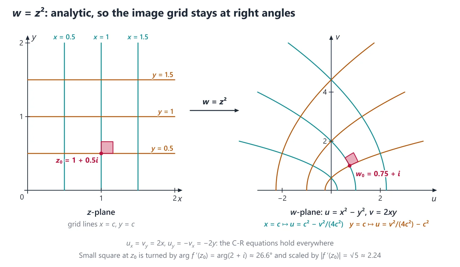
Idea: complex differentiability is much stronger than real differentiability: h can approach 0 from infinitely many directions, and the difference quotient must have the same limit along all of them. Geometrically, near z0 the map f acts like multiplication by the complex number f′(z0): a rotation through arg f′(z0) together with a stretch by the factor |f′(z0)|, so where f′(z0) ≠ 0 the map preserves angles (it is conformal).
Idea: analyticity is demanded on a whole neighbourhood because only then do the strong consequences follow: derivatives of all orders, a convergent Taylor series and Cauchy's theorem. Differentiability at a single point or along a line, as for |z|2 or x2 + iy2, gives none of them.
Examples: polynomials, ez, sin z and cos z are entire; z̄ is differentiable nowhere; |z|2 is differentiable only at z = 0 and so is analytic nowhere.
Why z̄ fails: for h = |h|eiφ the difference quotient of z̄ is h̄/h = e−2iφ, which equals 1 along the real axis (φ = 0) and −1 along the imaginary axis (φ = π/2), so no single limit exists.
3. Understanding the Cauchy-Riemann Equations
Why we need it: checking a limit in every direction is slow. We want a test that uses only the real part u(x, y) and the imaginary part v(x, y) and their ordinary partial derivatives, which we already know how to compute.
In words: ux = vy says that the rate of change of the real part in the x-direction equals the rate of change of the imaginary part in the y-direction; uy = −vx says the same for the other pair, with a minus sign. “Necessary” means: if f′ exists, these must hold. “Sufficient” means: if they hold and the four partials are continuous near the point, then f′ exists.
First example, slowly: f(z) = ez = ex(cos y + i sin y).
(1) Separate the parts: u = ex cos y and v = ex sin y.
(2) Differentiate: ux = ex cos y, uy = −ex sin y, vx = ex sin y, vy = ex cos y.
(3) Compare: ux = vy (both ex cos y) and uy = −vx (both −ex sin y), at every point.
(4) The four partials are continuous on all of ℂ, so the sufficient condition applies everywhere: ez is entire.
(5) Read off the derivative: f′ = ux + ivx = ex cos y + iex sin y = ez. Notice that the C-R test gives the derivative as a by-product.
Non-example: f(z) = |z|2 = x2 + y2, so u = x2 + y2, v = 0. Then ux = vy reads 2x = 0 and uy = −vx reads 2y = 0. Both hold only at the origin, so f is differentiable only at z = 0 and is analytic nowhere: a single point contains no disc.
Building up: (i) Let h → 0 along the real axis: the quotient tends to ux + ivx. (ii) Let h = ik → 0 along the imaginary axis: it tends to vy − iuy. (iii) Both are f′(z0), so equating real and imaginary parts gives the two equations (Standard Proofs, Theorem 1).
(iv) For the converse, continuity of the partials gives Δu = uxΔx + uyΔy + (small)·|h| by the mean value theorem, and similarly for v; the C-R equations then turn Δu + iΔv into (ux + ivx)(Δx + iΔy) + (small)·|h| (Standard Proofs, Theorem 2).
(v) The equations alone, at a single point, are not enough: √|xy| satisfies them at 0 without being differentiable there. Continuity of the partials, or a direct check of the limit, is what closes the gap.
Where it is used: in every “where is f differentiable or analytic” question, in proving that the real and imaginary parts are harmonic, in the Milne-Thomson method, and in Cauchy's theorem through Green's theorem.
4. Cauchy-Riemann Equations
Necessary condition: if f = u + iv is differentiable at z0 = x0 + iy0, then ux, uy, vx, vy exist at (x0, y0) and ux = vy, uy = −vx there; moreover f′(z0) = ux + ivx = vy − iuy.
Why it works: let h → 0 along the real axis (h = Δx); the quotient tends to ux + ivx. Let h → 0 along the imaginary axis (h = iΔy); it tends to (uy + ivy)/i = vy − iuy. Both limits equal f′(z0), and comparing real and imaginary parts gives ux = vy and vx = −uy (full proof in Standard Proofs, Section 1).
Sufficient condition: if u, v have continuous first partial derivatives in a neighbourhood of (x0, y0) and satisfy the C-R equations there, then f is analytic at z0.
Idea: continuity of the partials guarantees that u and v are differentiable as real functions, Δu ≈ uxΔx + uyΔy with an error small compared with |h|, and similarly for v. The C-R equations then turn this real linear approximation into a complex multiplication, Δu + iΔv ≈ (ux + ivx)(Δx + iΔy). Proof in Standard Proofs, Section 2.
Jacobian picture: with f′ = a + ib, the C-R equations say that the Jacobian matrix of (u, v) is [[ux, uy], [vx, vy]] = [[a, −b], [b, a]], which is |f′| times a rotation matrix. Its determinant ux2 + vx2 = |f′(z)|2 is the local area magnification.
Polar form: with z = reiθ, ur = (1/r)vθ and vr = −(1/r)uθ, and f′(z) = e−iθ(ur + ivr).
Complex form: the C-R equations are equivalent to ∂f/∂z̄ = 0, so an analytic function depends on z alone and not on z̄.
C-R alone is not sufficient: f(z) = √|xy| satisfies the C-R equations at 0 (all four partials are 0), but along y = mx the difference quotient is √|m|·|x|/(x(1 + im)), which depends on m, so f′(0) does not exist.
Example 1: Where is f(z) = x2 + iy2 differentiable, and where is it analytic?
u = x2, v = y2: ux = 2x, vy = 2y, uy = 0 = −vx. The partials are continuous and C-R holds iff x = y, so f is differentiable exactly on the line y = x. The line contains no open set, so f is analytic nowhere.
5. Derivation: Polar and Complex Forms of the C-R Equations
With x = r cos θ, y = r sin θ the chain rule gives ur = ux cos θ + uy sin θ and uθ = −rux sin θ + ruy cos θ, and the same formulas for v.
Substitute vx = −uy, vy = ux: vθ = −rvx sin θ + rvy cos θ = r(uy sin θ + ux cos θ) = rur, so ur = (1/r)vθ.
Similarly vr = vx cos θ + vy sin θ = −uy cos θ + ux sin θ = −(1/r)uθ.
Derivative: let h → 0 along the ray through z, h = eiθΔr; then Δf/h → (ur + ivr)/eiθ, so f′(z) = e−iθ(ur + ivr) = e−iθ(ur − (i/r)uθ).
Complex form: from x = (z + z̄)/2 and y = (z − z̄)/(2i) the chain rule gives ∂/∂z̄ = (1/2)(∂/∂x + i∂/∂y) and ∂/∂z = (1/2)(∂/∂x − i∂/∂y).
Then ∂f/∂z̄ = (1/2)[(ux − vy) + i(vx + uy)], which vanishes exactly when both C-R equations hold, and then ∂f/∂z = ux + ivx = f′(z).
Quick test: substitute x = (z + z̄)/2, y = (z − z̄)/(2i); if z̄ survives, f is not analytic. For example x2 + y2 = zz̄ has ∂/∂z̄ = z, which is zero only at 0.
Link: the C-R equations turn Green's theorem (Vector Analysis) into Cauchy's theorem in the next topic: the two double integrals in that proof vanish exactly because ux = vy and uy = −vx.
6. Understanding Harmonic Conjugates and the Milne-Thomson Method
Why we need it: in many problems only one real function is known, for example a temperature or a potential u(x, y). We ask two questions: is there an analytic f with Re f = u, and if so, how do we find it quickly?
In words: u is harmonic if its second partials are continuous and uxx + uyy = 0. A function v is a harmonic conjugate of u if u + iv is analytic, i.e. if the pair (u, v) satisfies the C-R equations. The word “conjugate” here has nothing to do with the complex conjugate z̄.
First example, slowly: u = x2 − y2.
(1) Check that u is harmonic: uxx = 2 and uyy = −2, so uxx + uyy = 0.
(2) The first C-R equation demands vy = ux = 2x. Integrate in y, treating x as a constant: v = 2xy + g(x), where g is an unknown function of x alone.
(3) The second C-R equation demands vx = −uy = 2y. From step (2), vx = 2y + g′(x). So g′(x) = 0 and g = C, a real constant.
(4) Hence v = 2xy + C and f = x2 − y2 + i(2xy + C) = (x + iy)2 + iC = z2 + iC.
(5) The Milne-Thomson shortcut gives the same in one line: ux(z, 0) = 2z and uy(z, 0) = 0, so f′(z) = 2z − i·0 and f = z2 + iC. Notice that it skips the partial integration and lands directly on a function of z.
Non-example: u = x2 + y2 has uxx + uyy = 4 ≠ 0. Trying anyway: vy = 2x gives v = 2xy + g(x), and vx = −uy = −2y then needs 2y + g′(x) = −2y, i.e. g′(x) = −4y, impossible for a function of x alone. A non-harmonic u is never the real part of an analytic function.
Building up: (i) Analytic f ⇒ u and v harmonic, by differentiating the C-R equations once more (Standard Proofs, Theorem 3). (ii) Conversely, on a simply connected domain the differential −uydx + uxdy is exact exactly when u is harmonic, so its integral is a conjugate v, unique up to adding a real constant.
(iii) Milne-Thomson: f′ = ux − iuy holds for all x, y; on the real axis z = x, and an analytic function is fixed by its values on a segment (identity theorem), so we may put x = z, y = 0. (iv) The constant is iC when u is given and a real C when v is given.
Where it is used: the standard “show u is harmonic and find f” question, the u − v and u + v variants, and later the complex potential of a two-dimensional flow (Fluid Dynamics) and steady temperature problems (Partial Differential Equations).
7. Harmonic Functions and Conjugates
Harmonic function: a real function u with continuous second partials satisfying Laplace's equation uxx + uyy = 0.
Theorem: if f = u + iv is analytic in a domain D, then u and v are harmonic in D; v is called a harmonic conjugate of u.
Why it works: uxx = (vy)x and uyy = (−vx)y, so uxx + uyy = vyx − vxy = 0. The mixed partials are equal because an analytic function has continuous derivatives of every order (Standard Proofs, Section 3).
Idea: on a simply connected domain every harmonic u has a harmonic conjugate, unique up to an additive real constant. On a domain with a hole this can fail: u = ln|z| is harmonic in ℂ − {0}, but its conjugate would be arg z, which is not single-valued there.
Order matters: if v is a conjugate of u, the conjugate of v is −u, not u, because −if = v − iu is analytic.
Orthogonality: the families of curves u = c1 and v = c2 cut each other at right angles where f′(z) ≠ 0.
Why it works: the normals to u = c1 and v = c2 are ∇u = (ux, uy) and ∇v = (vx, vy) = (−uy, ux), and their dot product is −uxuy + uyux = 0. In a two-dimensional flow these are the equipotential lines and the streamlines.
Finding the conjugate: from dv = vxdx + vydy = −uydx + uxdy, integrate this exact differential.
Why harmonicity is needed: the differential M dx + N dy with M = −uy, N = ux is exact iff ∂M/∂y = ∂N/∂x, i.e. −uyy = uxx, which is Laplace's equation. So the conjugate exists (locally) precisely because u is harmonic.
Milne-Thomson method:
1. Given u, compute φ1(x, y) = ux and φ2(x, y) = uy.
2. Then f′(z) = φ1(z, 0) − iφ2(z, 0) (replace x by z and y by 0).
3. Integrate: f(z) = ∫[φ1(z, 0) − iφ2(z, 0)] dz + iC.
4. If v is given instead, use f′(z) = vy(z, 0) + ivx(z, 0) and add a real constant C.
Why it works: f′(z) = ux − iuy holds identically in x and y, and on the real axis z = x, so f′(x) = φ1(x, 0) − iφ2(x, 0). When φ1(z, 0) − iφ2(z, 0) is an analytic expression in z, it agrees with f′ on a segment of the real axis, so by the identity theorem the two agree everywhere: replacing x by z and y by 0 is legitimate.
Polar Milne-Thomson (u given): from f′(z) = e−iθ(ur − (i/r)uθ), putting θ = 0 and r = z gives f′(z) = ur(z, 0) − (i/z)uθ(z, 0). Check: u = r2 cos 2θ gives f′(z) = 2z, so f = z2 + iC.
Link: harmonic functions solve Laplace's equation (Partial Differential Equations: steady temperature, electrostatic potential). In Fluid Dynamics the complex potential w = φ + iψ of a two-dimensional irrotational flow is analytic: φ is the velocity potential and its conjugate ψ is the stream function.
Example 2: Show that u = ex(x cos y − y sin y) is harmonic and find the analytic f = u + iv.
ux = ex(x cos y − y sin y + cos y) and uy = −ex(x sin y + sin y + y cos y). Differentiating again, uxx = ex(x cos y − y sin y + 2cos y) and uyy = −ex(x cos y + 2cos y − y sin y), so uxx + uyy = 0. Milne-Thomson: f′(z) = ez(z + 1) − i·0, so f(z) = zez + iC.
Example 3: Find the analytic function with u = x2 − y2 + x.
ux = 2x + 1, uy = −2y, so f′(z) = 2z + 1 and f(z) = z2 + z + iC; hence v = 2xy + y + C.
8. Understanding the Complex Logarithm and Branches
Why we need it: the equation ew = z has infinitely many solutions w for each z ≠ 0, because ew has period 2πi. To use log z, za or arg z in a formula (as in the PYQs on log z and ln(x2 + y2)) we must decide which solution we mean.
In words: log z = ln|z| + i arg z, where arg z is any angle of z, so the values differ by 2πik. A branch is a choice of the angle that varies continuously on a region; the principal branch Log z takes −π < Arg z < π and is defined on the plane with the half-line (−∞, 0] removed, the branch cut.
First example, slowly: find Log(−1 + i) and all values of log(−1 + i).
(1) Modulus: |−1 + i| = √2, so ln|z| = (1/2) ln 2.
(2) Angle: the point (−1, 1) is in the second quadrant on the line y = −x, so Arg z = 3π/4 (not −π/4, which is what tan−1(y/x) alone would suggest).
(3) Principal value: Log(−1 + i) = (1/2) ln 2 + 3πi/4 ≈ 0.3466 + 2.3562i.
(4) All values: log(−1 + i) = (1/2) ln 2 + i(3π/4 + 2kπ), k ∈ ℤ.
(5) Check: eLog z = √2(cos 3π/4 + i sin 3π/4) = √2(−1/√2 + i/√2) = −1 + i. The same idea gives ii = ei log i = e−π/2 − 2kπ, whose principal value e−π/2 ≈ 0.2079 is real.
Non-example: the real rule log(ab) = log a + log b fails for principal values. With a = b = −1: Log((−1)(−1)) = Log 1 = 0, but Log(−1) + Log(−1) = iπ + iπ = 2πi. The sum of the two angles, 2π, has left the range (−π, π], so the rule holds only up to a multiple of 2πi.
Building up: (i) On the cut plane, Log is the inverse of ew restricted to the strip −π < Im w < π. (ii) With u = ln r, v = θ the polar C-R equations hold, so Log z is analytic there with derivative 1/z (Past UPSC Questions, Example 10). (iii) Two branches differ by a constant 2πik, so every branch has derivative 1/z. (iv) Powers za = ea log z inherit the branches: one value for integer a, n values for a = 1/n.
Where it is used: conjugates such as arg z = tan−1(y/x) of ln|z|, answers of the form f = 2i log z + C, and later the branch points and keyhole contours of contour integration.
9. Elementary Functions
Exponential: ez = ex(cos y + i sin y); it is entire, never zero, and periodic with period 2πi.
Logarithm: log z = ln|z| + i arg z is multi-valued; the principal branch Log z (with −π < Arg z ≤ π) is analytic on ℂ minus the half-line (−∞, 0], with derivative 1/z.
Trigonometric: sin z = (eiz − e−iz)/(2i) and cos z = (eiz + e−iz)/2 are entire but unbounded; powers are defined by za = ea log z.
10. Choosing the Method
If asked whether f is differentiable or analytic at a point where f is defined piecewise (a special value at 0) → compute ux, uy, vx, vy there from the limit definition, check the C-R equations, then test lim f(h)/h along y = mx and along y = x2; two different limits prove that f′ does not exist.
If u and v are smooth formulas in x and y → the sufficient condition applies everywhere; solve the C-R equations as equations in x and y. Their solution set is where f is differentiable, and f is analytic only on the open part of that set.
If u (or v) is given and f is wanted → Milne-Thomson; if the conjugate itself is wanted, take the imaginary (or real) part of f, or integrate the exact differential dv = −uydx + uxdy.
If u or v is given in r and θ → the polar C-R equations or the polar Milne-Thomson formula, then write the answer in terms of z = reiθ.
If u − v or u + v is given → work with F = (1 + i)f or F = (1 − i)f, whose real part is the given combination.
If a relation such as v = u2, |f| = constant or arg f = constant is given → the constant-function test of the section on constrained analytic functions.
If a harmonic u is given on a domain with a hole → also check whether the conjugate is single-valued there (ln|z| on ℂ − {0} has none).
11. Common Mistakes
1. Concluding that f is differentiable because the C-R equations hold at a point. Without continuity of the partials, or a direct check of the limit, this proves nothing, as √|xy| at 0 shows.
2. Calling a function analytic on a line or at an isolated point where it is only differentiable (x2 + iy2 on y = x, |z|2 at 0). Analytic needs an open set.
3. Computing the partials at the origin by differentiating the formula valid only for z ≠ 0. At a special point use the limit definition, e.g. ux(0, 0) = limh→0 (u(h, 0) − u(0, 0))/h.
4. Losing the constant in Milne-Thomson: with u given, the constant in f is purely imaginary (iC) once Re f matches u; with v given, it is real.
5. Stating the harmonic conjugate of v as u; it is −u.
6. Leaving the final f in terms of x, y or z̄, or dropping the condition r > 0 and the factor 1/r in polar work.
Link: the Jacobian |f′(z)|2 is the area factor in a change of variables in a double integral (Calculus), and conformal maps keep angles because the Jacobian is a scaled rotation.
12. Worked Examples
Example 4: Find the real constants a, b, c for which f(z) = x + ay + i(bx + cy) is analytic, and express f in terms of z.
u = x + ay and v = bx + cy have continuous partials everywhere, so f is analytic iff the C-R equations hold.
ux = vy gives 1 = c, and uy = −vx gives a = −b.
Then f = x + ay + i(−ax + y) = (x + iy) − ia(x + iy) = (1 − ia)z, with a arbitrary.
Example 5: Show that u = x3 − 3xy2 + 3x2 − 3y2 + 1 is harmonic, and find a harmonic conjugate v and the analytic function f = u + iv.
ux = 3x2 − 3y2 + 6x and uy = −6xy − 6y, so uxx = 6x + 6 and uyy = −6x − 6. Hence uxx + uyy = 0 and u is harmonic.
Milne-Thomson: f′(z) = ux(z, 0) − iuy(z, 0) = 3z2 + 6z − i·0.
Integrating, f(z) = z3 + 3z2 + c; matching Re f with u gives c = 1 + iC, so f(z) = z3 + 3z2 + 1 + iC.
Taking the imaginary part, v = 3x2y − y3 + 6xy + C.
Example 6: Let f(z) = (x3 − y3 + i(x3 + y3))/(x2 + y2) for z ≠ 0 and f(0) = 0. Show that the C-R equations hold at 0 but f′(0) does not exist.
ux(0, 0) = lim (h3/h2)/h = 1, uy(0, 0) = lim (−k3/k2)/k = −1, vx(0, 0) = 1, vy(0, 0) = 1. So ux = vy and uy = −vx at 0.
Along the real axis, f(x)/x = (x3 + ix3)/x3 = 1 + i.
Along y = x, u = 0 and v = 2x3/(2x2) = x, so f(z)/z = ix/(x(1 + i)) = i/(1 + i) = (1 + i)/2.
The two limits differ, so f′(0) does not exist: the C-R equations are necessary but not sufficient (here the partials are not continuous at 0).
13. Polar Form, Logarithm and Constrained Analytic Functions
Polar Milne-Thomson: if v(r, θ) is given, the polar C-R equations give ur = (1/r)vθ and uθ = −rvr; integrate du = ur dr + uθ dθ, then write u + iv in terms of z = reiθ.
Sufficient conditions in polar form: if u, v and their first partials in r, θ are continuous in a domain not containing 0, and ur = (1/r)vθ, vr = −(1/r)uθ hold there, then f is analytic and f′(z) = e−iθ(ur + ivr).
Constant-function test: if f = u + iv is analytic in a domain D and Re f, Im f, |f| or arg f is constant, or u and v satisfy a differentiable relation v = φ(u), then f is constant. Method: put the relation into the C-R equations to get (1 + φ′(u)2)ux = 0 and (1 + φ′(u)2)uy = 0, so all first partials vanish and f′ = 0 on the connected set D.
Laplacian in z and z̄: ∇2 = ∂2/∂x2 + ∂2/∂y2 = 4∂2/∂z∂z̄. For f analytic this gives ∇2|f|2 = 4|f′(z)|2 and ∇2|f|p = p2|f|p−2|f′(z)|2 (where f ≠ 0), and log|g| is harmonic wherever g is analytic and non-zero, because locally log|g| = Re(log g).
Showing a combination is analytic: to prove that p + iq built from given harmonic functions is analytic, verify px = qy and py = −qx using Laplace's equation, and note that the partials are continuous (harmonic functions have continuous second partials).
When u − v or u + v is given: F = (1 + i)f = (u − v) + i(u + v) is analytic with real part u − v, and (1 − i)f has real part u + v; apply Milne-Thomson to F and divide by (1 + i) or (1 − i).
14. Past UPSC Questions Solved
Example 7 (UPSC 2015, 10 marks): Show that the function v(x, y) = ln(x2 + y2) + x + y is harmonic. Find its conjugate harmonic function u(x, y). Also, find the corresponding analytic function f(z) = u + iv in terms of z.
vx = 2x/(x2 + y2) + 1 and vy = 2y/(x2 + y2) + 1, so vxx = 2(y2 − x2)/(x2 + y2)2 and vyy = 2(x2 − y2)/(x2 + y2)2. Hence vxx + vyy = 0 for (x, y) ≠ (0, 0): v is harmonic in ℂ − {0}.
Milne-Thomson (v given): f′(z) = vy(z, 0) + ivx(z, 0) = 1 + i(2/z + 1).
Integrating, f(z) = z + i(z + 2 log z) + C = (1 + i)z + 2i log z + C, with C real.
With z = reiθ, 2i log z = 2i ln r − 2θ, so u = Re f = x − y − 2θ + C; check: Im f = x + y + 2 ln r = v.
Answer: u = x − y − 2 tan−1(y/x) + C and f(z) = (1 + i)z + 2i log z + C (analytic in any simply connected domain not containing 0, for a branch of log z).
Example 8 (UPSC 2020, 15 marks): If v(r, θ) = (r − 1/r) sin θ, r ≠ 0, then find an analytic function f(z) = u(r, θ) + iv(r, θ)
Polar C-R: ur = (1/r)vθ = (1/r)(r − 1/r)cos θ = (1 − 1/r2)cos θ, and uθ = −rvr = −r(1 + 1/r2)sin θ = −(r + 1/r)sin θ.
Integrating ur in r: u = (r + 1/r)cos θ + g(θ); then uθ = −(r + 1/r)sin θ + g′(θ), so g′ = 0 and g = C.
So f = (r + 1/r)cos θ + C + i(r − 1/r)sin θ = r(cos θ + i sin θ) + (1/r)(cos θ − i sin θ) + C = z + 1/z + C.
Answer: f(z) = z + 1/z + C (C real), analytic for z ≠ 0, with u = (r + 1/r)cos θ + C.
Example 9 (UPSC 2022, 10 marks): If f(z) = u + iv is an analytic function of z, and u − v = (cos x + sin x − e−y)/(2 cos x − ey − e−y), then find f(z) subject to the condition f(π/2) = 0.
Let F = (1 + i)f = (u − v) + i(u + v), which is analytic with real part U = u − v = N/D, where N = cos x + sin x − e−y and D = 2cos x − ey − e−y.
On y = 0: N = cos x + sin x − 1, D = 2cos x − 2, Nx = cos x − sin x, Dx = −2sin x, Ny = 1, Dy = 0.
Ux(x, 0) = (NxD − NDx)/D2 = (2 − 2cos x)/(4(1 − cos x)2) = 1/(2(1 − cos x)), and Uy(x, 0) = (NyD − NDy)/D2 = 1/D = −1/(2(1 − cos x)).
Milne-Thomson: F′(z) = Ux(z, 0) − iUy(z, 0) = (1 + i)/(2(1 − cos z)) = ((1 + i)/4)cosec2(z/2).
Integrating, F(z) = −((1 + i)/2)cot(z/2) + c, so f = F/(1 + i) = −(1/2)cot(z/2) + c′. The condition f(π/2) = 0 gives −(1/2)cot(π/4) + c′ = 0, so c′ = 1/2.
Answer: f(z) = (1/2)[1 − cot(z/2)].
Example 10 (UPSC 2023, 10 marks): State the sufficient conditions for a function f(z) = f(x + iy) = u(x, y) + iv(x, y) to be analytic in its domain. Hence, show that f(z) = log z is analytic in its domain and find df/dz.
Sufficient conditions: if u, v have continuous first partial derivatives in a domain D and satisfy ux = vy, uy = −vx at every point of D (in polar form ur = (1/r)vθ, vr = −(1/r)uθ, r > 0), then f = u + iv is analytic in D.
For the principal branch, z = reiθ with r > 0, −π < θ < π, and log z = ln r + iθ, so u = ln r, v = θ.
ur = 1/r, uθ = 0, vr = 0, vθ = 1 are continuous there, and ur = 1/r = (1/r)vθ, vr = 0 = −(1/r)uθ. Hence log z is analytic in ℂ minus the half-line (−∞, 0]; across the cut θ jumps by 2π, so this branch is not even continuous there (a branch with a different cut, such as 0 < θ < 2π, is analytic on the negative real axis).
df/dz = e−iθ(ur + ivr) = e−iθ/r = 1/(reiθ) = 1/z.
Answer: log z is analytic in ℂ − (−∞, 0] and d(log z)/dz = 1/z.
Example 11 (UPSC 2019, 10 marks): Suppose f(z) is analytic function on a domain D in ℂ and satisfies the equation Im f(z) = (Re f(z))2, z ∈ D. Show that f(z) is constant in D.
Write f = u + iv with v = u2 in D. The C-R equations give ux = vy = 2uuy and uy = −vx = −2uux.
Substituting the second into the first: ux = 2u(−2uux) = −4u2ux, i.e. (1 + 4u2)ux = 0.
Since 1 + 4u2 ≥ 1 > 0, ux = 0 in D, and then uy = −2uux = 0.
So f′ = ux + ivx = ux − iuy = 0 throughout D, and a function with zero derivative on a domain (a connected open set) is constant.
Answer: f is constant in D (its value c satisfies Im c = (Re c)2).
Example 12 (UPSC 2024, 10 marks): If w = f(z) is an analytic function of z, then show that (∂2/∂x2 + ∂2/∂y2) log |f′(z)| = 0.
Let g = f′, which is analytic (the derivative of an analytic function is analytic). The identity is meant where f′(z) ≠ 0, since log|f′| is undefined at zeros of f′.
Fix z0 with g(z0) ≠ 0 and a disc Δ about z0 on which g ≠ 0. On the simply connected disc, g′/g has a primitive h; adjusting the constant, eh = g on Δ, because (ge−h)′ = 0.
Then |g| = eRe h, so log|f′(z)| = Re h(z) on Δ, the real part of an analytic function.
The real part of an analytic function is harmonic, so (∂2/∂x2 + ∂2/∂y2) log|f′(z)| = 0 on Δ; z0 was arbitrary. (Check: log|g| = (h + h̄)/2 with ∂h/∂z̄ = 0 and ∂h̄/∂z = 0, so 4∂2(log|g|)/∂z∂z̄ = 0.)
Answer: ∇2 log|f′(z)| = 0 at every point where f′(z) ≠ 0.
Example 13 (UPSC 2024, 10 marks): If φ and ψ are functions of x and y satisfying Laplace equation, then show that f(z) = p + iq, i = √−1 is an analytic function, where p = ∂φ/∂y − ∂ψ/∂x and q = ∂φ/∂x + ∂ψ/∂y.
φ and ψ satisfy φxx + φyy = 0, ψxx + ψyy = 0 and have continuous second partials, so p = φy − ψx and q = φx + ψy have continuous first partials.
px = φyx − ψxx and qy = φxy + ψyy = φxy − ψxx; since φxy = φyx, px = qy.
py = φyy − ψxy = −φxx − ψxy, and −qx = −φxx − ψyx; since ψxy = ψyx, py = −qx.
The C-R equations hold and the partials are continuous, so by the sufficient condition f = p + iq is analytic.
Answer: f = p + iq is analytic wherever φ and ψ are harmonic.
15. Practice Exercises
Exercise 1 (basic): From the definition of the derivative, show that f(z) = 1/z is differentiable at every z ≠ 0 and find f′(z).
Answer: (1/(z + h) − 1/z)/h = −1/(z(z + h)) → −1/z2, so f′(z) = −1/z2.
Exercise 2 (basic): Is f(z) = x − iy + 2 analytic anywhere?
Answer: No. ux = 1 but vy = −1, so the C-R equations fail at every point; f = z̄ + 2 is differentiable nowhere.
Exercise 3 (basic): Show that u = x3 − 3xy2 is harmonic and find a harmonic conjugate.
Answer: uxx + uyy = 6x − 6x = 0; v = 3x2y − y3 + C, and f = z3 + iC.
Exercise 4 (standard): Find all points at which f(z) = x3 + i(1 − y)3 is differentiable. Is it analytic anywhere?
Answer: C-R needs 3x2 = −3(1 − y)2, so x = 0 and y = 1: f is differentiable only at z = i, with f′(i) = 0, and analytic nowhere.
Exercise 5 (standard): Find the analytic function f = u + iv with v = ex(x sin y + y cos y).
Answer: f′(z) = vy(z, 0) + ivx(z, 0) = (z + 1)ez, so f = zez + C (C real) and u = ex(x cos y − y sin y) + C.
Exercise 6 (standard): Find the analytic function whose real part is u = ln r + r cos θ (r > 0).
Answer: polar Milne-Thomson: f′(z) = ur(z, 0) − (i/z)uθ(z, 0) = 1/z + 1, so f = log z + z + iC, analytic in a cut plane such as ℂ − (−∞, 0].
Exercise 7 (standard): Show that f(z) = ez̄ is differentiable at no point.
Answer: u = ex cos y, v = −ex sin y; C-R needs cos y = 0 and sin y = 0 simultaneously, which never happens.
Exercise 8 (UPSC level): If f = u + iv is analytic and u + v = 2 sin 2x/(e2y + e−2y − 2 cos 2x), find f subject to f(π/2) = 0.
Answer: F = (1 − i)f has real part u + v = Re(cot z), so F = cot z + iC and the condition gives C = 0: f = ((1 + i)/2) cot z.
Exercise 9 (UPSC level): Prove that an analytic function with constant modulus on a domain is constant.
Answer: hint: differentiate u2 + v2 = c in x and y, use C-R to get (u2 + v2)ux = (u2 + v2)uy = 0, so f′ = 0 (the case c = 0 is trivial).
Exercise 10 (UPSC level): Let f(z) = xy2(x + iy)/(x2 + y4) for z ≠ 0 and f(0) = 0. Show that the C-R equations hold at 0 but f′(0) does not exist.
Answer: u and v vanish on both axes, so all four partials at 0 are 0. But (f(z) − f(0))/z = xy2/(x2 + y4) tends to 0 along every line y = mx and to 1/2 along x = y2.
Exercise 11 (UPSC level): Show that u = e−2xy sin(x2 − y2) is harmonic and find the analytic function f with Re f = u.
Answer: u = Im eiz2, so it is harmonic; Milne-Thomson gives f′ = 2z cos z2 + 2iz sin z2, hence f = −ieiz2 + iC.
| Form | Equations | Derivative |
|---|---|---|
| Cartesian | ux = vy, uy = −vx | f′ = ux + ivx |
| Polar | ur = (1/r)vθ, vr = −(1/r)uθ | f′ = e−iθ(ur + ivr) |
| Complex | ∂f/∂z̄ = 0 | f′ = ∂f/∂z |
| Milne-Thomson (u given) | f′(z) = ux(z, 0) − iuy(z, 0) | integrate in z |
| Milne-Thomson (v given) | f′(z) = vy(z, 0) + ivx(z, 0) | integrate in z |
Mains points
- A frequently asked question: show a given function satisfies the C-R equations at the origin but is not differentiable there; compute partials from the definition and then test the limit along y = mx or y = x2.
- Another standard question: given u or v (or u − v, u + v), show it is harmonic and find the analytic function by Milne-Thomson; state f in terms of z only.
- Prove the necessity of the C-R equations by letting h → 0 along the real and imaginary axes; for sufficiency, state the continuity of partials explicitly.
- Distinguish clearly between 'differentiable at a point' and 'analytic at a point'; f = |z|2 is the standard example.
- For u − v or u + v type questions, use F = (1 + i)f, whose real part is u − v.
Did you know?
- The C-R equations appeared in d'Alembert's work on fluid flow (1752), long before Cauchy and Riemann; in fluid dynamics u and v are the velocity potential and the stream function.
Cauchy's Theorem and Cauchy's Integral Formula
Cauchy's theorem says the integral of an analytic function around a closed contour in a simply connected domain is zero. Cauchy's integral formula recovers f and all its derivatives inside a contour from its boundary values, so an analytic function is infinitely differentiable. Consequences include Cauchy's inequality, Liouville's theorem, the fundamental theorem of algebra and the maximum modulus principle.
1. Understanding Contour Integrals
Why we need it: a complex function lives on a plane, not on a line, so “integrate from a to b” is meaningless until we say along which path. The contour integral is the complex version of a line integral, and ordinary definite integrals are the special case of a path along the real axis.
In words: a contour is a path z(t), a ≤ t ≤ b, made of finitely many smooth pieces, with a direction (from z(a) to z(b)). To integrate, replace z by z(t) and dz by z′(t) dt, and do an ordinary integral in t; the answer is a complex number. A closed contour ends where it starts, and ∮ is written for it; anticlockwise is the positive direction.
First example, slowly: ∮|z|=1 dz/z, the circle taken once anticlockwise.
(1) Parametrise: z = eit, 0 ≤ t ≤ 2π; as t increases the point moves anticlockwise once round the circle.
(2) Differentiate: dz = ieit dt.
(3) Substitute: f(z(t))z′(t) = (1/eit)·ieit = i.
(4) Integrate: ∫02π i dt = 2πi.
(5) Compare ∮|z|=1 z dz: the integrand becomes eit·ieit = ie2it, whose integral over [0, 2π] is 0. Notice that the closed integral of 1/z is not 0 although the path returns to its start: 1/z has no single-valued primitive on a curve round 0, while z has the primitive z2/2.
Non-example: path independence is not automatic. For z̄ from 0 to 1 + i the straight line gives 1 and the parabola y = x2 gives 1 + i/3 (Solved Problems, Problem 3). The two paths have the same ends but different values, because z̄ is not analytic and so has no primitive.
Building up: (i) The integral is linear, adds over pieces of the path, and changes sign when the direction is reversed; it does not depend on how the same oriented path is parametrised.
(ii) |∫ g(t) dt| ≤ ∫ |g(t)| dt gives the ML-inequality: |∫C f dz| ≤ (max of |f| on C) × (length of C).
(iii) If F′ = f on a region containing C, the chain rule gives d/dt F(z(t)) = f(z(t))z′(t), so ∫C f dz = F(end) − F(start), and every closed integral of f is 0. The value 2πi for 1/z therefore proves that 1/z has no primitive on ℂ − {0}.
Where it is used: every integral of this chapter starts here; the ML-inequality is the tool that kills the large arcs and small circles of contour integration, and the basic integral ∮ dz/(z − a) = 2πi is the seed of Cauchy's formula and of residues.
2. Contour Integrals
Definition: if C is given by z = z(t), a ≤ t ≤ b, then ∫C f(z) dz = ∫ab f(z(t))z′(t) dt.
Idea: the contour integral is the limit of sums ∑f(zk)Δzk along the path, where each Δzk is a small complex step with a direction. It depends only on the oriented path, not on the parametrisation chosen; reversing the direction changes its sign, and |∫C f dz| ≤ ∫C |f| |dz|.
ML-inequality: if |f(z)| ≤ M on C and C has length L, then |∫C f(z) dz| ≤ ML.
Idea: the estimate is crude but it is exactly what is needed to show that an integral over a large arc or a small circle tends to 0: if M falls faster than the length L grows, ML → 0. Proof in Standard Proofs, Section 4.
Basic integral: ∮|z−a|=r (z − a)n dz = 2πi if n = −1, and 0 for every other integer n.
Idea: every power (z − a)n with n ≠ −1 has the single-valued primitive (z − a)n+1/(n + 1), so its integral round a closed curve is 0. Only 1/(z − a) survives, because its primitive log(z − a) increases by 2πi each time the curve goes once round a. This single fact drives Cauchy's formula, Laurent series and residues.
Primitive: if f = F′ on a domain containing C, then ∫C f dz = F(end point) − F(initial point); in particular the integral over any closed contour is 0.
Idea: so a closed integral can be non-zero only when f has no primitive on the region. Cauchy's theorem says that on a simply connected domain an analytic f always has one, F(z) = ∫z0z f(ζ) dζ, the integral being independent of the path.
3. Understanding Cauchy's Theorem
Why we need it: parametrising every closed contour is laborious, and for complicated curves impossible. We want a theorem that says, from the function and the region alone, when a closed integral is 0.
In words: “f analytic in a simply connected domain D” means that f is differentiable at every point of an open connected set D that has no holes. “For every closed contour C in D” means that the whole curve must lie in D. The conclusion is ∮C f dz = 0, with no computation.
First example, slowly: ∮|z|=2 dz/(z − 3).
(1) Find the singular points of the integrand: only z = 3, where the denominator vanishes.
(2) Locate it: |3| = 3 > 2, so z = 3 lies outside the circle |z| = 2.
(3) Choose a domain: the disc D: |z| < 2.5 has no holes, contains the whole circle, and does not contain 3, so 1/(z − 3) is analytic in D.
(4) Apply the theorem: ∮|z|=2 dz/(z − 3) = 0. Notice that all the work was in locating the singular point; the theorem did the rest.
Non-example: ∮|z|=1 dz/z = 2πi. The function 1/z is analytic in the annulus 0 < |z| < 2, which contains the circle, but the annulus has a hole at 0. The hypothesis that fails is simple connectivity (equivalently, f must be analytic at every point inside C, and 0 is inside).
Building up: (i) If f′ is continuous, write ∮f dz as two real line integrals and apply Green's theorem; the double integrands are −vx − uy and ux − vy, both 0 by the C-R equations (Standard Proofs, Theorem 5). (ii) Goursat proved the same without assuming f′ continuous.
(iii) Consequences: in a simply connected domain the integral between two points is independent of the path, and F(z) = ∫z0z f dζ is a primitive. (iv) Deformation: a closed contour can be moved across any region where f is analytic without changing the integral, which reduces every closed integral to small circles round the singular points.
Where it is used: to show that integrals vanish, to justify deformation of contours, and as the first step in the proofs of Cauchy's integral formula, Laurent's theorem and the residue theorem.
4. Cauchy's Theorem
Cauchy–Goursat theorem: if f is analytic in a simply connected domain D, then ∮C f(z) dz = 0 for every simple closed contour C in D.
Idea: simply connected means the domain has no holes, so any closed curve in it can be shrunk to a point without leaving the domain. A hole may hide a singularity, and then the integral need not vanish (see the caution below). The conclusion also holds for closed contours that cross themselves, since they split into simple loops.
Green's theorem proof (assuming f′ continuous): ∮f dz = ∮(u dx − v dy) + i∮(v dx + u dy) = ∬(−vx − uy) dx dy + i∬(ux − vy) dx dy = 0 by the C-R equations. Goursat removed the continuity assumption.
Why the hypothesis: Green's theorem needs continuous partial derivatives, hence the extra assumption that f′ is continuous (the version proved in Standard Proofs, Section 5). Goursat's proof subdivides a triangle into smaller and smaller triangles and uses only the existence of f′; it then follows that f′ is automatically continuous.
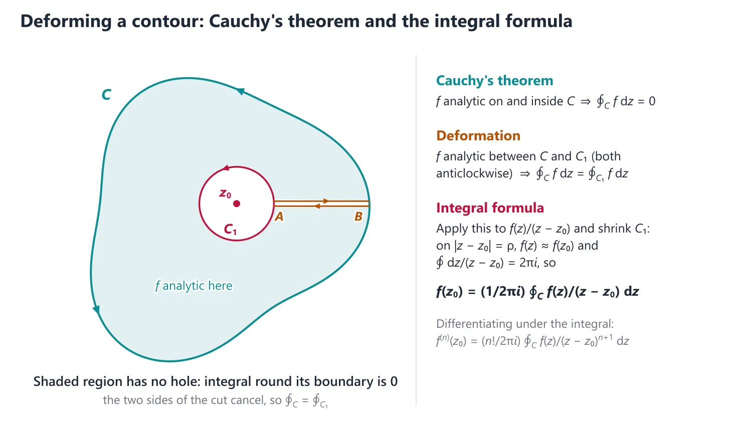
Deformation of contours: if C1 lies inside C and f is analytic on both curves and in the region between them, then ∮C f dz = ∮C1 f dz (both anticlockwise).
Why it works: join C to C1 by a cross-cut AB. The closed path C, then AB, then C1 clockwise, then BA bounds a region with no hole on which f is analytic, so its integral is 0. The integrals along AB and BA cancel, leaving ∮C f dz − ∮C1 f dz = 0.
Several holes: in the same way, if C1, ..., Ck are disjoint contours inside C and f is analytic in the region between them, ∮C f dz = ∑∮Cj f dz. This is the step that leads to the residue theorem.
Morera's theorem (converse): if f is continuous in a domain D and ∮C f dz = 0 for every closed contour C in D, then f is analytic in D.
Idea: if every closed integral vanishes, F(z) = ∫z0z f(ζ) dζ is well defined and F′ = f, so F is analytic; the derivative of an analytic function is analytic, hence f is analytic (Standard Proofs, Section 10). Its main use is to prove analyticity of limits and integrals, e.g. a uniform limit of analytic functions is analytic.
Caution: simple connectivity matters: 1/z is analytic in 0 < |z| < 2, but ∮|z|=1 dz/z = 2πi ≠ 0.
5. Understanding Cauchy's Integral Formula
Why we need it: Cauchy's theorem says nothing when the integrand has a singular point inside C, which is exactly the interesting case. For integrands of the form f(z)/(z − a) with f analytic, we want the actual value.
In words: “f analytic inside and on C” means that f itself has no singular point in the closed region bounded by C; the only trouble in f(z)/(z − a) is the factor 1/(z − a). Then the integral equals 2πi times the value f(a). More generally the power (z − a)n+1 in the denominator produces 2πi f(n)(a)/n!.
First example, slowly: ∮|z|=3 cos πz/(z − 1) dz, and then the same with (z − 1)2.
(1) Match the pattern f(z)/(z − a): here a = 1 and f(z) = cos πz.
(2) Check the hypotheses: cos πz is entire, so it is analytic inside and on |z| = 3; and |1| < 3, so a is inside.
(3) Apply the formula: the integral is 2πi f(1) = 2πi cos π = −2πi.
(4) With (z − 1)2 = (z − 1)1+1 we have n = 1, so the integral is 2πi f′(1)/1! = 2πi(−π sin π) = 0.
(5) Notice the bookkeeping: the exponent of (z − a) is one more than the order of the derivative, and the factorial of that order divides.
Non-example: for ∮|z|=2 dz/((z − 1)(z + 1)) it is tempting to take a = 1 and f(z) = 1/(z + 1), giving 2πi·(1/2) = πi. This is wrong, because f has a singular point at −1, which is also inside |z| = 2. Splitting by partial fractions gives πi − πi = 0, the correct value.
Building up: (i) Shrink C to a small circle round a (deformation). (ii) On that circle f(z) is close to f(a), and ∮ f(a)/(z − a) dz = 2πi f(a) by the basic integral. (iii) The remainder is at most 2π·max|f(z) − f(a)|, which tends to 0 as the circle shrinks (Standard Proofs, Theorem 6). (iv) Differentiating under the integral sign gives the derivative formulas, so an analytic function has derivatives of every order.
Where it is used: evaluating integrals with one or two poles inside the contour (a standard 10-mark question), proving Taylor's theorem, and through Cauchy's inequality, Liouville's theorem.
6. Understanding Liouville's Theorem and the Maximum Modulus Principle
Why we need it: the integral formula controls an analytic function so tightly that strong global conclusions follow. Typical questions ask to show that an entire function with some bound is constant, or to find the largest value of |f| on a closed disc.
In words: Liouville: if f is entire and one number M satisfies |f(z)| ≤ M for every z in ℂ, then f is constant. Maximum modulus: a non-constant analytic f has no point inside its domain where |f| is largest; on a closed bounded region the maximum of |f| is reached on the boundary.
First example, slowly: find the maximum and minimum of |ez| on the closed disc |z| ≤ 1.
(1) ez is entire and not constant, so its maximum modulus on the disc is attained on the circle |z| = 1.
(2) |ez| = |exeiy| = ex, and on the circle x = cos θ.
(3) cos θ is largest (= 1) at θ = 0, so the maximum is e, at z = 1.
(4) ez never vanishes, so the minimum modulus principle also applies: the minimum is on the circle too, e−1 at z = −1. Notice that at the centre |e0| = 1 lies strictly between them.
Non-example: sin z is entire and |sin x| ≤ 1 for real x, but Liouville does not apply: |sin(iy)| = sinh|y| → ∞, so sin z is not bounded on ℂ. Similarly f(z) = z on |z| ≤ 1 has minimum modulus 0 at the centre, an interior point, because it has a zero there.
Building up: (i) Cauchy's inequality |f′(z0)| ≤ M/r holds on every circle; letting r → ∞ gives f′ ≡ 0 (Standard Proofs, Theorems 7 and 8). (ii) If a polynomial p had no zero, 1/p would be bounded and entire, hence constant: the fundamental theorem of algebra (Theorem 9).
(iii) Gauss's mean value property says f(z0) is the average of f over any circle round z0; an average cannot exceed its largest value unless all values are equal, which forces |f| constant near a maximum point and then f constant (Theorem 14).
Where it is used: questions of the type “entire with Re f bounded (or |f| ≤ A|z|n) implies constant (or polynomial)”, the fundamental theorem of algebra, and maximum or minimum of |f| on a closed region.
7. Cauchy's Integral Formula and Consequences
Integral formula: if f is analytic inside and on a simple closed contour C (taken anticlockwise) and z0 is inside C, then f(z0) = (1/2πi)∮C f(z)/(z − z0) dz.
Idea: the values of an analytic function on a closed curve completely determine its values inside, something with no analogue for real differentiable functions. Picture: shrink C to a tiny circle round z0 (deformation), on which f(z) ≈ f(z0); the basic integral then gives f(z0)·2πi. Proof in Standard Proofs, Section 6.
Derivatives: under the same hypotheses f has derivatives of all orders at z0, and f(n)(z0) = (n!/2πi)∮C f(z)/(z − z0)n+1 dz.
Derivation: differentiate the integral formula with respect to z0 under the integral sign. Since d/dz0 (z − z0)−1 = (z − z0)−2, and n differentiations give n!(z − z0)−(n+1), the formula for f(n)(z0) follows. The step is justified because C stays at a positive distance from z0, so the difference quotients of the integrand converge uniformly on C.
Working form: ∮C f(z)/(z − a)n+1 dz = 2πi f(n)(a)/n! for a inside C. Consequence: an analytic function is infinitely differentiable, whereas a real function such as x|x| has a first derivative but no second at 0.
Cauchy's inequality: if f is analytic inside and on |z − z0| = r and |f| ≤ M there, then |f(n)(z0)| ≤ n!M/rn.
Why it works: apply the ML-inequality to the derivative formula on the circle |z − z0| = r: |f(n)(z0)| ≤ (n!/2π)·(M/rn+1)·2πr = n!M/rn (Standard Proofs, Section 7).
Liouville's theorem: a bounded entire function is constant.
Idea: if |f| ≤ M on ℂ, Cauchy's inequality with n = 1 gives |f′(z0)| ≤ M/r for every r, and letting r → ∞ gives f′ ≡ 0 (Standard Proofs, Section 8). The hypothesis is boundedness on all of ℂ: sin z is bounded on ℝ but not on ℂ, since |sin iy| = sinh |y|.
Generalised Liouville: if f is entire and |f(z)| ≤ A|z|n for |z| ≥ R0, then f is a polynomial of degree at most n, because Cauchy's inequality on |z| = r gives |f(k)(0)| ≤ k!Arn/rk → 0 as r → ∞ for every k > n.
Fundamental theorem of algebra: every non-constant polynomial has a zero in ℂ; otherwise 1/p(z) would be a bounded entire function, hence constant.
Gauss's mean value theorem: f(z0) = (1/2π)∫02π f(z0 + reiθ) dθ, the value at the centre is the average over the circle.
Derivation: put z = z0 + reiθ, dz = ireiθ dθ in the integral formula: f(z0) = (1/2πi)∫02π f(z0 + reiθ)·ireiθ dθ/(reiθ) = (1/2π)∫02π f(z0 + reiθ) dθ. Taking real parts, every harmonic function also has this mean value property.
Maximum modulus principle: if f is analytic and non-constant in a domain D, then |f| has no maximum in D. If f is continuous on a closed bounded region and analytic inside it, max |f| is attained on the boundary.
Idea: by the mean value theorem, |f(z0)| ≤ the average of |f| over every small circle round z0. If |f(z0)| were the largest value, |f| would have to equal |f(z0)| on all those circles, so |f| would be constant near z0, which forces f to be constant (Standard Proofs, Section 14). Picture: the graph of |f| has no peaks, only saddles.
Minimum modulus: if in addition f has no zero in D, |f| has no minimum in D.
Why it works: apply the maximum modulus principle to 1/f, which is analytic because f ≠ 0. The extra hypothesis is essential: f(z) = z on |z| ≤ 1 has its minimum modulus 0 at the centre.
Link: Cauchy's theorem is Green's theorem (Vector Analysis) combined with the C-R equations, and its independence of path matches conservative fields (curl F = 0) there. The mean value property and the maximum principle reappear for harmonic functions and Laplace's equation (Partial Differential Equations).
Link: the fundamental theorem of algebra, proved here with Liouville, is what guarantees that every complex square matrix has an eigenvalue (Linear Algebra).
8. Choosing the Method
If f is analytic inside and on C → ∮C f dz = 0 by Cauchy's theorem; just verify that every singularity lies outside C.
If the integrand is g(z)/(z − a) with g analytic and a inside C → 2πi g(a); if it is g(z)/(z − a)n+1 → 2πi g(n)(a)/n!.
If two or more singular points lie inside C → split by partial fractions, or surround each point by a small circle (deformation) and apply the integral formula in each; the residue theorem of the next topic does the same in one step.
If the integrand is not analytic (z̄, |z|, Re z, x2 + iy) → no theorem applies; parametrise the path.
If an entire function is bounded, or grows at most like |z|n → Liouville or generalised Liouville via Cauchy's inequality.
If the maximum or minimum of |f| on a closed region is asked → maximum (minimum) modulus principle: search only the boundary, and for the minimum first check that f has no zero inside.
9. Common Mistakes
1. Applying Cauchy's theorem when a singularity lies inside C, e.g. writing ∮|z|=1 dz/z = 0. Always locate the singular points relative to C first.
2. Dropping the n! or using the wrong power in the derivative formula: (z − a)n+1 in the denominator goes with f(n)(a)/n!, so (z − a)3 gives 2πi f″(a)/2.
3. Choosing g(z) in g(z)/(z − a) so that g itself has a singularity inside C. All other singular factors must either lie outside C or be split off first.
4. Ignoring orientation: a clockwise contour gives the negative of the anticlockwise value.
5. Using Liouville for a function bounded only on the real axis (sin z, cos z), or the minimum modulus principle for a function with a zero inside.
6. Quoting Morera without checking continuity of f, or Cauchy's theorem on a domain with holes.
10. Worked Examples
Example 1: Evaluate ∮|z|=2 ez/(z − 1) dz.
f(z) = ez is entire and z = 1 lies inside |z| = 2, so the integral is 2πi·f(1) = 2πie.
Example 2: Evaluate ∮|z|=3 e2z/(z + 1)4 dz.
With f(z) = e2z and n = 3, f‴(z) = 8e2z, so the integral is (2πi/3!)·f‴(−1) = (2πi/6)·8e−2 = 8πie−2/3.
Example 3: Evaluate ∮C dz/(z2 − 1), where C is |z − 1| = 1.
Only z = 1 lies inside C (since |−1 − 1| = 2 > 1). Write the integrand as [1/(z + 1)]/(z − 1); by the integral formula the value is 2πi·1/2 = πi.
Example 4: Show that an entire function f with |f(z)| ≤ A|z| for all z is of the form f(z) = cz.
By Cauchy's inequality on |z| = R, |f″(0)| ≤ 2·AR/R2 → 0, and the same holds at every point, so f″ ≡ 0 and f(z) = a + cz. Since |f(0)| ≤ 0, a = 0.
Example 5: Evaluate ∮C (z2 − z + 1)/(z − 1) dz when C is (i) |z| = 1/2, (ii) |z| = 2.
(i) The only singularity z = 1 lies outside |z| = 1/2, so the integrand is analytic inside and on C and the integral is 0 by Cauchy's theorem.
(ii) z = 1 lies inside |z| = 2. With f(z) = z2 − z + 1 (entire), Cauchy's integral formula gives 2πi·f(1) = 2πi·1 = 2πi.
Example 6: Evaluate ∮|z|=3 (sin πz2 + cos πz2)/((z − 1)(z − 2)) dz.
Partial fractions: 1/((z − 1)(z − 2)) = 1/(z − 2) − 1/(z − 1). Both 1 and 2 lie inside |z| = 3.
With f(z) = sin πz2 + cos πz2 (entire), the integral is 2πi[f(2) − f(1)] by Cauchy's integral formula.
f(2) = sin 4π + cos 4π = 1 and f(1) = sin π + cos π = −1, so the integral is 2πi(1 + 1) = 4πi.
Example 7: Let f be entire with Re f(z) ≤ M for all z. Show that f is constant.
Put g(z) = ef(z), which is entire. |g(z)| = eRe f(z) ≤ eM, so g is bounded.
By Liouville's theorem g is constant, so 0 = g′(z) = f′(z)ef(z).
Since ef(z) ≠ 0, f′ ≡ 0 on ℂ, and f is constant.
11. Integrals along Arcs and Functions from Boundary Values
Analytic integrand: if f has a primitive F on a domain containing the arc (true for polynomials, ez, sin z), then ∫C f dz = F(end) − F(start) for every path, with no need to parametrise.
Non-analytic integrand (z̄, Re z, |z|2, Re(z2)): the value depends on the path, so parametrise: on y = x2 put z = t + it2, dz = (1 + 2it) dt; on a circle put z = reiθ.
Analytic function from boundary values on |z| = 1: put z = eiθ, so cos θ = (z + 1/z)/2, sin θ = (z − 1/z)/(2i), cos 2θ = (z2 + z−2)/2, and simplify the given expression to a function of z. If the result is analytic inside and on |z| = 1, it is the required function.
Uniqueness: if two functions analytic inside and on C agree on C, their difference is zero on C and hence, by the maximum modulus principle, zero inside C.
Example 8 (UPSC 2020, 10 marks): Evaluate the integral ∫C (z2 + 3z) dz counterclockwise from (2, 0) to (0, 2) along the curve C, where C is the circle |z| = 2.
z2 + 3z is entire with primitive F(z) = z3/3 + 3z2/2, so the integral does not depend on the path and equals F(2i) − F(2).
F(2i) = (2i)3/3 + 3(2i)2/2 = −8i/3 − 6 and F(2) = 8/3 + 6 = 26/3.
Parametrising z = 2eiθ, 0 ≤ θ ≤ π/2, gives the same value, as Cauchy's theorem requires.
Answer: ∫C (z2 + 3z) dz = −44/3 − 8i/3.
Example 9 (UPSC 2024, 20 marks): Find the function which is analytic inside and on the circle C : z = eiθ, 0 ≤ θ ≤ 2π and has the value [(a2 − 1) cos θ + i(a2 + 1) sin θ]/(a4 − 2a2 cos 2θ + 1), on the circumference of C, where a2 > 1.
On C, z = eiθ, so cos θ + i sin θ = z and cos θ − i sin θ = 1/z.
Numerator: (a2 − 1)cos θ + i(a2 + 1)sin θ = a2(cos θ + i sin θ) − (cos θ − i sin θ) = a2z − 1/z = (a2z2 − 1)/z.
Denominator: a4 − 2a2cos 2θ + 1 = a4 − a2(z2 + 1/z2) + 1 = (a2 − z2)(a2 − 1/z2) = (a2 − z2)(a2z2 − 1)/z2.
Dividing (a2z2 − 1 ≠ 0 on |z| = 1 since a2 > 1), the boundary value is ((a2z2 − 1)/z)·z2/((a2 − z2)(a2z2 − 1)) = z/(a2 − z2).
f(z) = z/(a2 − z2) has poles only at z = ±a with |±a| > 1, so it is analytic inside and on C and takes the given values on C; by the uniqueness remark above it is the only such function.
Answer: f(z) = z/(a2 − z2).
12. Practice Exercises
Exercise 1 (basic): Evaluate ∫C z2 dz along the straight segment from 0 to 1 + i, by parametrising.
Answer: z = t(1 + i), dz = (1 + i) dt, integral = (1 + i)3/3 = (−2 + 2i)/3, the same as F(1 + i) − F(0) with F = z3/3.
Exercise 2 (basic): Evaluate ∮|z|=1 cos z/(z − 2) dz.
Answer: 0, by Cauchy's theorem, since z = 2 lies outside |z| = 1.
Exercise 3 (basic): Evaluate ∮|z|=1 e3z/z dz.
Answer: 2πi·e0 = 2πi.
Exercise 4 (standard): Evaluate ∮|z|=2 z/((z − 1)(z − 3)) dz.
Answer: only z = 1 is inside; with f(z) = z/(z − 3), the value is 2πi f(1) = 2πi(−1/2) = −πi.
Exercise 5 (standard): Evaluate ∮|z|=1 sin z/z4 dz.
Answer: n = 3: 2πi f‴(0)/3! = 2πi(−cos 0)/6 = −πi/3.
Exercise 6 (standard): Evaluate ∮C dz/(z2 + 1), where C is the circle |z − i| = 1.
Answer: z = i is inside and z = −i (at distance 2 from i) is outside; with f = 1/(z + i), the value is 2πi/(2i) = π.
Exercise 7 (standard): Find the maximum of |z2 + 1| on the closed disc |z| ≤ 1 and where it is attained.
Answer: on |z| = 1, |e2iθ + 1| = 2|cos θ|, so the maximum is 2, at z = ±1.
Exercise 8 (UPSC level): Using Cauchy's integral formula, evaluate ∮|z|=2 ez/(z2 + 1) dz.
Answer: 1/(z2 + 1) = (1/2i)[1/(z − i) − 1/(z + i)], both points inside, so the value is π(ei − e−i) = 2πi sin 1.
Exercise 9 (UPSC level): Let f be entire with |f(z)| ≤ 1 + √|z| for all z. Prove that f is constant.
Answer: hint: Cauchy's inequality on |z − z0| = r gives |f′(z0)| ≤ (1 + √(|z0| + r))/r → 0 as r → ∞, so f′ ≡ 0.
Exercise 10 (UPSC level): Evaluate ∮|z|=3 e2z/((z + 1)2(z − 2)) dz.
Answer: surround −1 and 2 by small circles. At 2: 2πi e4/9. At −1 (n = 1, f = e2z/(z − 2)): 2πi f′(−1) = 2πi(−7e−2/9). Total 2πi(e4 − 7e−2)/9 ≈ 37.455i.
| Theorem | Hypothesis | Conclusion |
|---|---|---|
| Cauchy–Goursat | f analytic in a simply connected domain D, C closed in D | ∮C f dz = 0 |
| Morera | f continuous in D, ∮C f dz = 0 for all closed C | f analytic in D |
| Integral formula | f analytic inside and on C, z0 inside C | f(n)(z0) = (n!/2πi)∮ f/(z − z0)n+1 dz |
| Liouville | f entire and bounded | f constant |
| Maximum modulus | f analytic, non-constant in D | |f| has no maximum in D |
Mains points
- Integral evaluation by Cauchy's integral formula is very frequently asked: identify which singular points lie inside the contour, split by partial fractions if needed, and apply the derivative formula for repeated factors.
- State Cauchy's theorem with the hypothesis of a simply connected domain (or f analytic inside and on C); quote Cauchy–Goursat when f′ is not assumed continuous.
- Liouville's theorem and its use to prove the fundamental theorem of algebra are standard theory questions; write the Cauchy inequality step explicitly.
- Variants of Liouville (|f(z)| ≤ A|z|n ⇒ f is a polynomial of degree ≤ n; Re f bounded ⇒ f constant using ef) appear often.
- Always draw the contour and mark the singular points; examiners give credit for showing which points are inside.
Did you know?
- Cauchy's integral formula means an analytic function is completely fixed inside a circle by its values on the circle, a rigidity with no analogue for real differentiable functions.
Power Series, Taylor's Series and Laurent's Series
A power series converges inside a disc of radius R = 1/lim sup |an|1/n and its sum is analytic there. Conversely every analytic function equals its Taylor series in the largest disc about z0 free of singularities. In an annulus an analytic function has a Laurent series with negative powers, whose coefficient a−1 is the residue.
1. Understanding the Radius of Convergence
Why we need it: a polynomial is a finite sum of powers; a power series ∑an(z − z0)n is an infinite one. An infinite sum means something only where it converges, so before using a series we must know for which z it converges.
In words: there is a number R, 0 ≤ R ≤ ∞, the radius of convergence, such that the series converges absolutely when |z − z0| < R and diverges when |z − z0| > R. So the region of convergence is a disc centred at z0, plus possibly some points of its boundary circle. lim sup |an|1/n is the largest limit of subsequences of |an|1/n; when lim |an/an+1| exists it equals R.
First example, slowly: ∑n≥1 nzn/3n.
(1) Identify the coefficients: an = n/3n, all non-zero, so the ratio form may be tried.
(2) Form the ratio: an/an+1 = (n/3n)·(3n+1/(n + 1)) = 3n/(n + 1).
(3) Take the limit: 3n/(n + 1) → 3, so R = 3. The series converges absolutely for |z| < 3 and diverges for |z| > 3.
(4) Test the circle separately: if |z| = 3, the n-th term has modulus n, which does not tend to 0, so the series diverges at every point of |z| = 3. Notice that the formula for R never decides the boundary; that always needs a separate argument.
Non-example: ∑ n!zn has an/an+1 = 1/(n + 1) → 0, so R = 0: it converges only at z = 0 and defines no analytic function. Being written as a power series does not by itself make something a function on a disc.
Building up: (i) The root test applied to ∑|an||z − z0|n gives the Cauchy–Hadamard formula. (ii) Abel's lemma (convergence at z1 forces absolute convergence for every z nearer to z0) explains why the region is a disc. (iii) The differentiated series ∑nan(z − z0)n−1 has the same R, because n1/n → 1, and it is the derivative of the sum (Standard Proofs, Theorem 16); repeating, an = f(n)(z0)/n!.
Where it is used: short questions asking for R, the region of validity of every Taylor expansion, and the annuli in which Laurent series converge.
2. Power Series
Radius of convergence (Cauchy–Hadamard): for ∑an(z − z0)n, 1/R = lim sup |an|1/n, or R = lim |an/an+1| when this limit exists.
Derivation: apply the root test to ∑|an||z − z0|n: lim sup (|an||z − z0|n)1/n = |z − z0|·lim sup |an|1/n, which is less than 1 exactly when |z − z0| < R. If it exceeds 1, infinitely many terms have modulus greater than 1, so the terms do not tend to 0 and the series diverges. The ratio form comes the same way from the ratio test: |an+1(z − z0)n+1|/|an(z − z0)n| → |z − z0|/R.
Caution: the ratio form needs the limit to exist. For ∑z2n/4n every other coefficient is 0, so put w = z2: ∑(w/4)n converges for |w| < 4, i.e. |z| < 2, which agrees with the root form, lim sup |ak|1/k = 1/2.
Behaviour: the series converges absolutely for |z − z0| < R, uniformly on every closed disc |z − z0| ≤ r < R, and diverges for |z − z0| > R.
Why a disc (Abel's lemma): if the series converges at z1, its terms are bounded there, |an(z1 − z0)n| ≤ K. For |z − z0| < |z1 − z0| put ρ = |z − z0|/|z1 − z0| < 1; then |an(z − z0)n| ≤ Kρn, and comparison with a geometric series gives absolute convergence. So the set of convergence is always a disc, plus possibly some points of its boundary circle.
On the circle: anything can happen. ∑zn diverges at every point of |z| = 1, ∑zn/n2 converges at every point, and ∑zn/n converges at every point except z = 1.
Power series representation: the sum f(z) of a power series is analytic in |z − z0| < R, can be differentiated term by term any number of times, and an = f(n)(z0)/n!. Hence the representation is unique.
Idea: differentiating term by term multiplies an by n, and n1/n → 1, so the derived series has the same radius R (Standard Proofs, Section 16). Putting z = z0 after k differentiations leaves k!ak = f(k)(z0), which is why the coefficients, and hence the series, are unique.
3. Understanding Taylor's Series
Why we need it: to compute values, locate and count zeros, and later read off residues, we want to write an analytic function as a power series about a chosen point.
In words: if f is analytic on the whole disc |z − z0| < R, then f(z) equals ∑f(n)(z0)(z − z0)n/n! at every point of that disc. The series works out to the nearest singular point of f and no further, so the radius is exactly the distance from z0 to the nearest singularity.
First example, slowly: expand f(z) = 1/(3 − z) about z0 = 1.
(1) Shift the centre: put w = z − 1, so z = 1 + w and 3 − z = 2 − w.
(2) Bring it to geometric form: 1/(2 − w) = (1/2)·1/(1 − w/2).
(3) Expand: for |w/2| < 1, 1/(1 − w/2) = ∑(w/2)n, so f = ∑n=0∞ wn/2n+1.
(4) Return to z: 1/(3 − z) = ∑(z − 1)n/2n+1, valid for |z − 1| < 2.
(5) Check two ways: the only singularity, z = 3, is at distance 2 from the centre, matching the radius; and a1 should be f′(1) = 1/(3 − 1)2 = 1/4, which is 1/22. Notice that no derivative was computed to get the series; uniqueness guarantees it is the Taylor series.
Non-example: Log z has no Taylor series about z0 = 0: it is not analytic at 0 (not even defined there). About z0 = 1 it does: Log z = ∑n≥1 (−1)n+1(z − 1)n/n for |z − 1| < 1. The condition that fails at 0 is analyticity at the centre.
Building up: (i) Write Cauchy's formula on a circle inside the disc and expand 1/(ζ − z) as a geometric series in (z − z0)/(ζ − z0); uniform convergence allows term-by-term integration, and the coefficients come out as f(n)(z0)/n! (Standard Proofs, Theorem 11).
(ii) A zero of order m means f = (z − z0)mg with g(z0) ≠ 0; continuity of g makes the zero isolated. (iii) Hence two analytic functions that agree on a set with a limit point in the domain agree everywhere (identity theorem).
Where it is used: series questions with a stated region, finding the order of zeros and poles, residues from series, identity-theorem questions, and the Milne-Thomson justification.
4. Taylor's Series
Taylor's theorem: if f is analytic in |z − z0| < R, then f(z) = ∑n=0∞ f(n)(z0)(z − z0)n/n! for every z in that disc. The radius of convergence is at least the distance from z0 to the nearest singularity of f.
Idea: the proof (Standard Proofs, Section 11) puts the geometric series 1/(ζ − z) = ∑(z − z0)n/(ζ − z0)n+1 into Cauchy's integral formula. It works on any circle |ζ − z0| = ρ inside the domain, so the series converges out to the nearest singularity. This explains a real puzzle: 1/(1 + x2) is smooth on all of ℝ, yet its Maclaurin series 1 − x2 + x4 − ... has radius 1, because of the poles at ±i.
Contrast with real analysis: e−1/x2 (with value 0 at 0) has all derivatives 0 at x = 0, so its Maclaurin series is identically 0 and does not represent it. In the complex plane this cannot happen: an analytic function always equals its Taylor series near each point.
Standard series: ez = ∑zn/n!, sin z = z − z3/3! + z5/5! − ..., cos z = 1 − z2/2! + z4/4! − ... (all for every z); 1/(1 − z) = ∑zn and Log(1 + z) = z − z2/2 + z3/3 − ... for |z| < 1.
Method: almost never compute f(n) directly. Build the series from the standard ones by substitution, multiplication, division, differentiation or integration; uniqueness guarantees that whatever power series you obtain is the Taylor series. For example 1/(1 − z)2 = d/dz (1/(1 − z)) = ∑(n + 1)zn, and Log(1 + z) = ∫0z dζ/(1 + ζ).
Zeros: z0 is a zero of order m if f(z0) = ... = f(m−1)(z0) = 0 and f(m)(z0) ≠ 0; then f(z) = (z − z0)mg(z) with g analytic and g(z0) ≠ 0. Zeros of a non-zero analytic function are isolated.
Why zeros are isolated: g is continuous and g(z0) ≠ 0, so g ≠ 0 on some disc round z0, and there f = (z − z0)mg vanishes only at z0. The only alternative is that every derivative vanishes at z0, and then the Taylor series is 0 and f ≡ 0 near z0.
Identity theorem: if f and g are analytic in a domain D and f = g on a set having a limit point in D, then f ≡ g in D.
Idea: an analytic function is rigid: its values on any small arc, or on any convergent sequence of points, fix it everywhere in the domain. The limit point must lie in D: sin(1/z) vanishes at the points 1/(nπ) → 0 without being identically 0, because 0 is not in its domain of analyticity.
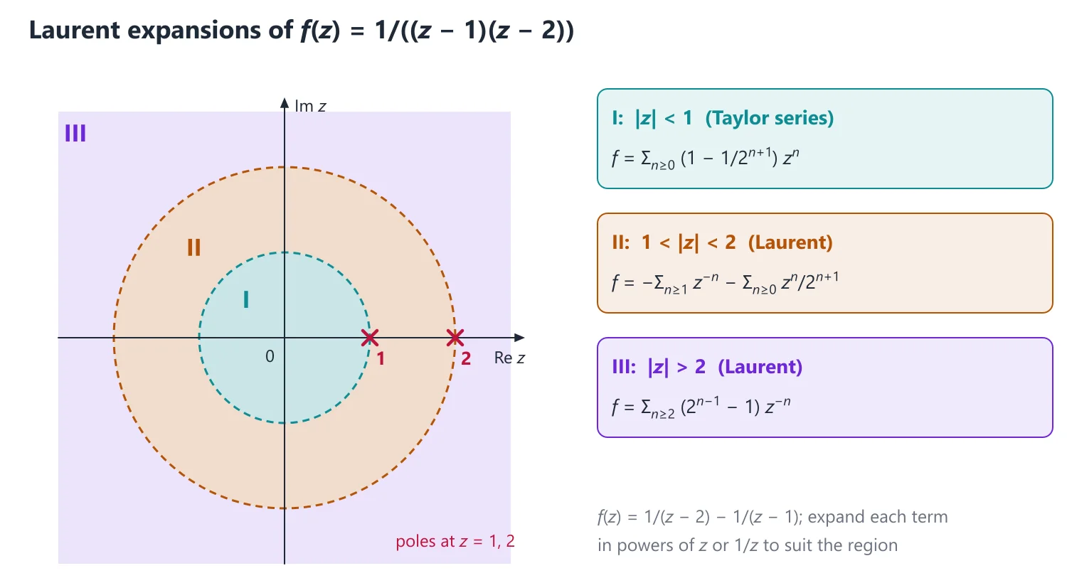
Example 1: Expand f(z) = 1/((z − 1)(z − 2)) in a Taylor series about z = 0.
f = 1/(z − 2) − 1/(z − 1) = 1/(1 − z) − (1/2)·1/(1 − z/2). For |z| < 1, f(z) = ∑n=0∞ (1 − 1/2n+1)zn; the radius is 1, the distance to the singularity z = 1.
5. Understanding Laurent's Series
Why we need it: near a singular point, such as 0 for 1/z or e1/z, no Taylor series exists, yet we still want a series describing f close to that point. The answer is a series valid in a ring that goes round the singular point.
In words: if f is analytic in the annulus r < |z − z0| < R (the point z0 itself may be bad), then f = ∑n=−∞∞ an(z − z0)n there, with both positive and negative powers. The negative powers form the principal part. For a given annulus the series is unique, but a different annulus about the same centre has a different series.
First example, slowly: f(z) = 1/(z(1 − z)) about z0 = 0, in 0 < |z| < 1 and in |z| > 1.
(1) Partial fractions: 1/(z(1 − z)) = 1/z + 1/(1 − z).
(2) In 0 < |z| < 1 we have |z| < 1, so 1/(1 − z) = 1 + z + z2 + ..., and f = 1/z + 1 + z + z2 + ....
(3) In |z| > 1 that series diverges, so write 1/(1 − z) = −(1/z)·1/(1 − 1/z) = −(1/z + 1/z2 + 1/z3 + ...), valid because |1/z| < 1.
(4) Add: f = 1/z − 1/z − 1/z2 − ... = −1/z2 − 1/z3 − ... for |z| > 1.
(5) Compare the coefficients of 1/z: it is 1 in the punctured disc, which is the residue at 0, and 0 in |z| > 1, which is the sum of the residues at 0 and 1 (1 + (−1)). Notice that both series are correct, each in its own ring.
Non-example: Log z has no Laurent series in 0 < |z| < 1. The punctured disc goes round 0, and no branch of the logarithm is analytic (even continuous) on a full circle round 0, since its imaginary part would have to increase by 2π. The hypothesis that fails is analyticity on the whole annulus.
Building up: (i) Apply Cauchy's formula to the region between two circles of the annulus; the outer circle produces the positive powers and the inner circle the negative powers (section on the derivation below). (ii) Integrating the series term by term round a circle shows that each coefficient is a fixed integral, so the series is unique and any method (partial fractions, substitution) gives it. (iii) In particular ∮ f dz = 2πia−1 over a circle in the annulus.
Where it is used: the frequent “expand in the regions ...” question, classification of isolated singularities from the principal part, and residues at essential singularities.
6. Laurent's Series
Laurent's theorem: if f is analytic in the annulus r < |z − z0| < R, then f(z) = ∑n=−∞∞ an(z − z0)n there, where an = (1/2πi)∮C f(ζ)/(ζ − z0)n+1 dζ for any circle C: |ζ − z0| = ρ with r < ρ < R. The expansion is unique.
Idea: an annulus has a hole that may contain singularities, and positive powers alone cannot describe a function that blows up inside the hole; negative powers are needed. The positive powers come from the outer boundary circle and the negative powers from the inner one, as the derivation below shows. See the figure above: 1/((z − 1)(z − 2)) has a different Laurent series in each of the regions |z| < 1, 1 < |z| < 2 and |z| > 2.
Parts: ∑n≥0 an(z − z0)n is the regular (analytic) part and ∑n≥1 a−n(z − z0)−n is the principal part.
Idea: when the annulus is a punctured disc 0 < |z − z0| < R, the principal part carries all the singular behaviour of f at z0, and the type of singularity is read from it (next topic).
Residue link: a−1 = (1/2πi)∮C f(z) dz, so ∮C f dz = 2πia−1.
Caution: in an annulus such as 1 < |z| < 2 the coefficient a−1 gives ∮ f dz over a circle in that annulus, which is 2πi times the sum of the residues inside the circle. It is the residue at z0 only when the annulus is a punctured disc about z0.
Method:
1. Split f into partial fractions.
2. For each term 1/(z − a), write it as a geometric series in z/a if |z| < |a| in the region, and in a/z if |z| > |a|.
Why it works: 1/(z − a) = −(1/a)·1/(1 − z/a) = −∑n=0∞ zn/an+1, valid when |z/a| < 1; and 1/(z − a) = (1/z)·1/(1 − a/z) = ∑n=0∞ an/zn+1, valid when |a/z| < 1. Each term is expanded in whichever ratio has modulus less than 1 throughout the region.
3. For an expansion about z0 ≠ 0, first substitute w = z − z0.
4. Combine the series and state the region of validity.
Example 2: Expand f(z) = 1/((z − 1)(z − 2)) in (i) 1 < |z| < 2, (ii) |z| > 2, (iii) 0 < |z − 1| < 1.
(i) −1/(z − 1) = −(1/z)·1/(1 − 1/z) = −∑n=1∞ z−n and 1/(z − 2) = −∑n=0∞ zn/2n+1, so f = −∑n=1∞ z−n − ∑n=0∞ zn/2n+1.
(ii) 1/(z − 2) = ∑n=1∞ 2n−1/zn and −1/(z − 1) = −∑n=1∞ 1/zn, so f = ∑n=2∞ (2n−1 − 1)/zn.
(iii) With w = z − 1, f = 1/(w(w − 1)) = −(1/w)(1 + w + w2 + ...) = −1/(z − 1) − 1 − (z − 1) − (z − 1)2 − .... The residue at z = 1 is −1.
Example 3: e1/z = 1 + 1/z + 1/(2!z2) + 1/(3!z3) + ... for |z| > 0; the principal part is infinite and the residue at 0 is 1.
7. Derivation: Laurent's Series from Cauchy's Integral Formula
Let r < r1 < |z − z0| < r2 < R, and let C1, C2 be the circles of radii r1, r2 about z0, both anticlockwise.
Cauchy's integral formula for the region between them (cross-cut argument) gives f(z) = (1/2πi)∮C2 f(ζ)/(ζ − z) dζ − (1/2πi)∮C1 f(ζ)/(ζ − z) dζ.
On C2, |z − z0| < |ζ − z0|, so 1/(ζ − z) = ∑n≥0 (z − z0)n/(ζ − z0)n+1; integrating term by term gives the non-negative powers with an = (1/2πi)∮C2 f(ζ)/(ζ − z0)n+1 dζ.
On C1, |ζ − z0| < |z − z0|, so −1/(ζ − z) = 1/((z − z0) − (ζ − z0)) = ∑n≥1 (ζ − z0)n−1/(z − z0)n; this gives the negative powers with a−n = (1/2πi)∮C1 f(ζ)(ζ − z0)n−1 dζ.
The integrands are analytic in the annulus, so by deformation both coefficient integrals may be taken over any one circle |ζ − z0| = ρ, r < ρ < R; then both formulas are the single formula an = (1/2πi)∮ f(ζ)/(ζ − z0)n+1 dζ for all integers n. The geometric series converge uniformly on the circles, which justifies the term-by-term integration.
Uniqueness: if f = ∑bn(z − z0)n in the annulus, multiply by (z − z0)−k−1 and integrate round |z − z0| = ρ; by the basic integral only n = k survives, giving bk = ak. So any method that produces a series of this form, such as partial fractions, gives the Laurent series.
8. Choosing the Method
If f is analytic at z0 and a series in powers of z − z0 is asked → Taylor series from the standard series; the radius is the distance from z0 to the nearest singularity.
If f is rational and an annulus is specified → partial fractions, then expand each term in z/a or a/z according to the region (see Why it works above).
If the expansion is about z0 ≠ 0 → put w = z − z0 and write each factor z − a = w − (a − z0); the regions are then decided by |w| compared with |a − z0|.
If f is e1/z, sin(1/z), zke1/z or similar → substitute 1/z into the standard series directly; the expansion is valid for |z| > 0.
If f is a quotient such as 1/(z2 sin z) or cot z near 0 → series division (or undetermined coefficients) for the first few terms.
If no region is stated → list the distances of the singularities from z0; they cut the plane into the discs and annuli in which separate expansions exist, and give each one.
9. Common Mistakes
1. Using R = lim |an/an+1| for a series with missing powers (∑z2n, ∑zn!); use the root form or substitute w = z2.
2. Expanding 1/(z − a) in powers of z/a in a region where |z| > |a|, where that series diverges. Check that each ratio has modulus less than 1 throughout the region.
3. Not stating the region of validity; the same function has different series in different annuli, and the answer is incomplete without the region.
4. Calling a−1 of the series valid in 1 < |z| < 2 the residue at 0; f may even be analytic at 0.
5. Expanding about z0 but writing the final answer in powers of z instead of z − z0.
6. Taking the radius of a Taylor series from the real behaviour of f instead of from its complex singularities (1/(1 + x2) has R = 1).
Link: radius of convergence, uniform convergence and the Weierstrass M-test are the same tools as for real power series and series of functions (Real Analysis).
Link: on the unit circle the Laurent coefficients an = (1/2π)∫02π f(eiθ)e−inθ dθ are exactly the complex Fourier coefficients of f(eiθ), the Fourier series used for boundary value problems (Partial Differential Equations).
10. Worked Examples
Example 4: Find the radius of convergence of ∑(n!/nn)zn.
With an = n!/nn, an/an+1 = (n!/nn)·((n + 1)n+1/(n + 1)!) = (n + 1)n/nn = (1 + 1/n)n.
This tends to e, so R = lim |an/an+1| = e.
The series converges absolutely for |z| < e and diverges for |z| > e.
Example 5: Expand f(z) = 1/z in a Taylor series about z = 2 and find the region of validity.
Write 1/z = 1/(2 + (z − 2)) = (1/2)·1/(1 + (z − 2)/2).
For |z − 2| < 2, the geometric series gives 1/z = ∑n=0∞ (−1)n(z − 2)n/2n+1.
The radius is 2, the distance from 2 to the only singularity z = 0, as Taylor's theorem predicts.
Example 6: Find the Laurent series of f(z) = ez/(z − 1)2 about z = 1 and the residue there.
Put w = z − 1, so ez = e·ew = e(1 + w + w2/2! + w3/3! + ...).
Then f = e(1/w2 + 1/w + 1/2 + w/6 + ...), i.e. f(z) = e/(z − 1)2 + e/(z − 1) + e/2 + e(z − 1)/6 + ..., valid for 0 < |z − 1| < ∞.
The principal part has two terms, so z = 1 is a pole of order 2, and the residue (coefficient of 1/(z − 1)) is e.
11. Repeated and Quadratic Factors, Coefficient Integrals, Identity Theorem
Repeated factor: for |w| < 1, 1/(1 + w)2 = ∑n=0∞ (−1)n(n + 1)wn and 1/(1 − w)2 = ∑n=0∞ (n + 1)wn (differentiate the geometric series).
Quadratic factor: 1/(1 + z2) = ∑n=0∞ (−1)nz2n for |z| < 1 and ∑n=0∞ (−1)nz−2n−2 for |z| > 1; keep the term as (Bz + C)/(z2 + 1) in partial fractions instead of splitting over ±i.
Coefficients as integrals: when the unit circle lies in the annulus, the Laurent coefficient formula becomes an = (1/2π)∫02π f(eiθ)e−inθ dθ. This proves expansions such as e(c/2)(z − 1/z) = ∑n=−∞∞ Jn(c)zn, with Jn(c) = (1/2π)∫02π cos(nθ − c sin θ) dθ (Bessel coefficients).
Symmetric functions: if f(1/z) = f(z), then a−n = an, and the expansion can be written a0 + ∑n=1∞ an(zn + z−n).
Identity theorem in use: if an analytic function vanishes at distinct points zk → z0 with z0 in the domain (for example at 1/k → 0), it vanishes identically.
Polynomial test: an entire f is a polynomial of degree at most n − 1 iff f(n) ≡ 0, because its Taylor series about 0 converges on all of ℂ and ak = f(k)(0)/k! = 0 for k ≥ n.
12. Past UPSC Questions Solved
Example 7 (UPSC 2014, 10 marks): Expand in Laurent series the function f(z) = 1/[z2(z − 1)] about z = 0 and z = 1.
About z = 0, for 0 < |z| < 1: 1/(z − 1) = −(1 + z + z2 + ...), so f = −1/z2 − 1/z − 1 − z − z2 − ...; the residue at 0 is −1.
About z = 0, for |z| > 1: 1/(z − 1) = (1/z)∑n=0∞ z−n, so f = ∑n=3∞ 1/zn = 1/z3 + 1/z4 + ....
About z = 1, put w = z − 1, so f = 1/(w(1 + w)2). For 0 < |w| < 1: f = (1/w)∑n=0∞ (−1)n(n + 1)wn = 1/(z − 1) − 2 + 3(z − 1) − 4(z − 1)2 + ...; the residue at 1 is 1.
About z = 1, for |w| > 1: 1/(1 + w)2 = (1/w2)(1 + 1/w)−2, so f = ∑n=0∞ (−1)n(n + 1)/(z − 1)n+3 = 1/(z − 1)3 − 2/(z − 1)4 + 3/(z − 1)5 − ....
Answer: 0 < |z| < 1: −∑n=−2∞ zn; |z| > 1: ∑n=3∞ z−n; 0 < |z − 1| < 1: ∑n=0∞ (−1)n(n + 1)(z − 1)n−1; |z − 1| > 1: ∑n=0∞ (−1)n(n + 1)(z − 1)−n−3.
Example 8 (UPSC 2018, 15 marks): Find the Laurent's series which represent the function 1/((1 + z2)(z + 2)) when
(i) |z| < 1
(ii) 1 < |z| < 2
(iii) |z| > 2
Partial fractions: 1/((1 + z2)(z + 2)) = (1/5)[1/(z + 2) + (2 − z)/(1 + z2)] (check at z = 0: (1/5)(1/2 + 2) = 1/2).
Pieces: 1/(z + 2) = ∑ (−1)nzn/2n+1 for |z| < 2 and ∑ (−1)n2n/zn+1 for |z| > 2; 1/(1 + z2) = ∑ (−1)nz2n for |z| < 1 and ∑ (−1)n/z2n+2 for |z| > 1 (all sums from n = 0).
(i) |z| < 1: f = (1/5)[∑ (−1)nzn/2n+1 + (2 − z)∑ (−1)nz2n] = 1/2 − z/4 − 3z2/8 + ..., a Taylor series.
(ii) 1 < |z| < 2: f = (1/5)[∑ (−1)nzn/2n+1 + (2 − z)∑ (−1)n/z2n+2] = (1/5)[... + 1/z3 + 2/z2 − 1/z + 1/2 − z/4 + z2/8 − ...].
(iii) |z| > 2: f = (1/5)[∑ (−1)n2n/zn+1 + (2 − z)∑ (−1)n/z2n+2]; the 1/z and 1/z2 terms cancel, leaving f = 1/z3 − 2/z4 + ....
Answer: the three series above, f = (1/5)[A(z) + (2 − z)B(z)] with A, B the expansions of 1/(z + 2) and 1/(1 + z2) valid in the given region.
Example 9 (UPSC 2022, 10 marks): Expand f(z) = 1/((z − 1)2(z − 3)) in a Laurent series valid for the regions (i) 0 < |z − 1| < 2 and (ii) 0 < |z − 3| < 2.
(i) w = z − 1, 0 < |w| < 2: z − 3 = w − 2, so f = 1/(w2(w − 2)) = −(1/(2w2))·1/(1 − w/2) = −∑n=0∞ wn−2/2n+1.
So f = −1/(2(z − 1)2) − 1/(4(z − 1)) − 1/8 − (z − 1)/16 − ...; z = 1 is a pole of order 2 with residue −1/4.
(ii) t = z − 3, 0 < |t| < 2: z − 1 = t + 2, so f = 1/(t(t + 2)2) = (1/(4t))(1 + t/2)−2 = ∑n=0∞ (−1)n(n + 1)tn−1/2n+2.
So f = 1/(4(z − 3)) − 1/4 + 3(z − 3)/16 − (z − 3)2/8 + ...; z = 3 is a simple pole with residue 1/4.
Answer: (i) f = −∑n=0∞ (z − 1)n−2/2n+1; (ii) f = ∑n=0∞ (−1)n(n + 1)(z − 3)n−1/2n+2.
Example 10 (UPSC 2026, 15 marks): Prove that cosh(z + 1/z) = a0 + ∑n=1∞ an(zn + 1/zn), where an = (1/(2π)) ∫02π cos nθ cosh(2 cos θ) dθ, for n = 0, 1, 2, ….
g(z) = cosh(z + 1/z) is analytic in 0 < |z| < ∞, so it has a Laurent series ∑n=−∞∞ anzn there, with an = (1/2πi)∮|z|=1 g(z)/zn+1 dz.
On |z| = 1 put z = eiθ: z + 1/z = 2cos θ and dz = ieiθ dθ, so an = (1/2π)∫02π cosh(2cos θ)(cos nθ − i sin nθ) dθ.
Under θ → 2π − θ, cosh(2cos θ) is unchanged and sin nθ changes sign, so ∫02π cosh(2cos θ) sin nθ dθ = 0 and an = (1/2π)∫02π cos nθ cosh(2cos θ) dθ.
cos(−nθ) = cos nθ gives a−n = an (equivalently g(1/z) = g(z)); grouping the terms n and −n gives cosh(z + 1/z) = a0 + ∑n=1∞ an(zn + 1/zn).
Answer: the expansion holds for all z ≠ 0, with an = (1/(2π))∫02π cos nθ cosh(2cos θ) dθ, n = 0, 1, 2, ....
Example 11 (UPSC 2017, 15 marks): For a function f : ℂ → ℂ and n ≥ 1, let f(n) denote the nth derivative of f and f(0) = f. Let f be an entire function such that for some n ≥ 1, f(n)(1/k) = 0 for all k = 1, 2, 3, .... Show that f is a polynomial.
g = f(n) is entire and g(1/k) = 0 for k = 1, 2, 3, ...; the zeros 1/k are distinct and converge to 0, a point of the domain ℂ.
Zeros of a non-zero analytic function are isolated, so by the identity theorem g ≡ 0 on ℂ.
The Taylor series f(z) = ∑ akzk, ak = f(k)(0)/k!, converges on all of ℂ; for k ≥ n, f(k) = g(k−n) ≡ 0, so ak = 0.
Answer: f(z) = a0 + a1z + ... + an−1zn−1, a polynomial of degree at most n − 1.
13. Practice Exercises
Exercise 1 (basic): Find the radius of convergence of ∑n≥1 zn/(n2n).
Answer: an/an+1 = 2(n + 1)/n → 2, so R = 2.
Exercise 2 (basic): Find the radius of convergence of ∑(n!)2zn/(2n)!.
Answer: an/an+1 = (2n + 1)(2n + 2)/(n + 1)2 → 4, so R = 4.
Exercise 3 (basic): Write the first three non-zero terms of the Maclaurin series of zez2 and its region of validity.
Answer: z + z3 + z5/2 + ..., valid for all z.
Exercise 4 (standard): Expand 1/z2 in a Taylor series about z = 1 and state the region.
Answer: 1/(1 + w)2 with w = z − 1 gives ∑n≥0 (−1)n(n + 1)(z − 1)n, for |z − 1| < 1.
Exercise 5 (standard): Expand sin z in a Taylor series about z = π/4.
Answer: sin(π/4 + w) = (cos w + sin w)/√2, so sin z = (1/√2)[1 + (z − π/4) − (z − π/4)2/2! − (z − π/4)3/3! + (z − π/4)4/4! + ...], valid for all z.
Exercise 6 (standard): Expand f(z) = z/((z − 1)(z − 3)) in a Laurent series valid in 1 < |z| < 3.
Answer: f = −(1/2)/(z − 1) + (3/2)/(z − 3) = −(1/2)∑n≥1 z−n − (1/2)∑n≥0 zn/3n.
Exercise 7 (standard): Find the Laurent series of sin z/z3 about 0, the nature of the singularity and the residue.
Answer: 1/z2 − 1/6 + z2/120 − ... for z ≠ 0: a pole of order 2 with residue 0.
Exercise 8 (UPSC level): Expand f(z) = 1/(z(z − 1)(z − 2)) in Laurent series valid in (i) 0 < |z| < 1, (ii) 1 < |z| < 2, (iii) |z| > 2.
Answer: f = 1/(2z) − 1/(z − 1) + 1/(2(z − 2)). (i) 1/(2z) + ∑n≥0 (1 − 1/2n+2)zn; (ii) −1/(2z) − ∑n≥2 z−n − ∑n≥0 zn/2n+2; (iii) ∑n≥3 (2n−2 − 1)z−n = 1/z3 + 3/z4 + 7/z5 + ....
Exercise 9 (UPSC level): Find the Laurent series of e2z/(z − 1)3 about z = 1 (first four terms) and the residue at z = 1.
Answer: with w = z − 1, e2e2w/w3 = e2[1/w3 + 2/w2 + 2/w + 4/3 + ...]; a pole of order 3 with residue 2e2.
Exercise 10 (UPSC level): Show that no function f analytic in |z| < 1 satisfies f(1/n) = (−1)n/n for n = 2, 3, 4, ....
Answer: hint: on the points 1/(2k) → 0, f agrees with z, so f(z) = z by the identity theorem; but then f(1/3) = 1/3, not −1/3.
| Function | Series | Valid for |
|---|---|---|
| ez | 1 + z + z2/2! + z3/3! + ... | all z |
| sin z | z − z3/3! + z5/5! − ... | all z |
| cos z | 1 − z2/2! + z4/4! − ... | all z |
| 1/(1 − z) | 1 + z + z2 + ... | |z| < 1 |
| 1/(1 − z) | −(1/z + 1/z2 + 1/z3 + ...) | |z| > 1 |
| Log(1 + z) | z − z2/2 + z3/3 − ... | |z| < 1 |
| (1 + z)α (principal) | 1 + αz + α(α − 1)z2/2! + ... | |z| < 1 |
Mains points
- The most common question: expand a rational function such as 1/((z − 1)(z − 2)) or z/((z + 1)(z + 2)) in Laurent series valid in each given region; write the region next to every expansion.
- When the centre is not 0 (for example about z = 1 or z = i), substitute w = z − z0 first; forgetting this is the most frequent error.
- State Taylor's and Laurent's theorems with full hypotheses (analytic in the disc or annulus) and the coefficient formula; short proof questions use the Cauchy integral formula with a geometric series.
- Radius-of-convergence questions for complex power series use the root or ratio formula; mention behaviour on the boundary only if asked.
- Use Laurent series to classify singularities and read off residues, especially at essential singularities such as z2e1/z or sin(1/z).
Did you know?
- Why does the real function 1/(1 + x2), smooth on all of ℝ, have a Taylor series about 0 that converges only for |x| < 1? Its complex singularities at ±i are at distance 1 from the origin.
Singularities and Cauchy's Residue Theorem
An isolated singularity is removable, a pole of order m, or essential, according as the principal part of the Laurent series has no terms, finitely many, or infinitely many. The residue is the coefficient a−1, computed by limit formulas at poles. Cauchy's residue theorem turns a closed contour integral into 2πi times the sum of residues inside.
1. Understanding Isolated Singularities
Why we need it: a closed integral depends only on how f behaves near its singular points inside the contour. Before computing anything we must recognise, quickly and correctly, what kind of bad point each one is.
In words: z0 is an isolated singularity if f is analytic in some punctured disc 0 < |z − z0| < r but not at z0. Then f has a Laurent series there, and the principal part decides the type: no negative powers means removable (the hole can be filled), finitely many means a pole (f blows up like 1/(z − z0)m), infinitely many means essential (wild behaviour).
First example, slowly: classify the singular points of f(z) = sin z/(z2(z − π)).
(1) Zeros of the denominator: z = 0 (order 2, from z2) and z = π (order 1). These are the only candidates.
(2) Zeros of the numerator at those points: sin z has a simple zero at 0 (sin z = z − z3/6 + ...) and a simple zero at π (its derivative cos π = −1 ≠ 0).
(3) At 0: denominator order 2 minus numerator order 1 = 1, so a simple pole. Indeed sin z/z2 = 1/z − z/6 + ... and 1/(z − π) → −1/π, so the principal part is −1/(πz).
(4) At π: 1 − 1 = 0, so removable: sin z/(z − π) → cos π = −1, hence f(z) → −1/π2, a finite limit.
(5) Notice the method: compare the orders of the zeros of numerator and denominator found from Taylor series, never just the visible factors.
Non-example: 0 is a singular point of 1/sin(1/z) but not an isolated one, since the poles 1/(nπ) crowd into every disc round 0; and 0 is a branch point of Log z, which is not analytic in any punctured disc round 0. Neither has a Laurent series about 0, so neither is removable, a pole or essential.
Building up: (i) Riemann: if f is bounded near z0, every principal-part coefficient is at most Mρn for every small ρ, hence 0, so the singularity is removable (Standard Proofs, Theorem 12). (ii) A pole of order m is the same as f = φ/(z − z0)m with φ analytic and φ(z0) ≠ 0 (Theorem 17); this is why zero orders can simply be subtracted. (iii) If neither holds the singularity is essential, and Casorati–Weierstrass says f comes arbitrarily close to every value near it.
Where it is used: the short “find and classify all singularities” question, choosing the right residue formula, and deciding which points a contour integral must account for.
2. Classification of Singularities
Singular point: z0 is a singular point of f if f is not analytic at z0 but every neighbourhood of z0 contains points where f is analytic. It is isolated if f is analytic in some punctured disc 0 < |z − z0| < r.
Idea: isolated means that z0 is the only trouble spot in a small punctured disc, so a Laurent series in 0 < |z − z0| < r exists. That Laurent series, and in particular its principal part, is what classifies the singularity.
Removable singularity: the principal part is zero; equivalently limz→z0 f(z) exists finitely (Riemann: it suffices that f is bounded near z0). Example: (sin z)/z at 0.
Idea: the hole can simply be filled in: defining f(z0) = lim f(z) makes f analytic at z0. Riemann's theorem (Standard Proofs, Section 12) needs only boundedness near z0, or even (z − z0)f(z) → 0.
Pole of order m: the principal part has finitely many terms, with a−m ≠ 0 and a−n = 0 for n > m; equivalently lim (z − z0)mf(z) is finite and non-zero. Then |f(z)| → ∞ as z → z0. A pole of order 1 is a simple pole.
Idea: near a pole f behaves like a−m/(z − z0)m: it blows up at a definite rate. The order is the unique m for which (z − z0)mf(z) has a finite non-zero limit; a smaller power leaves the limit infinite, a larger one makes it 0 (Standard Proofs, Section 17).
Essential singularity: the principal part has infinitely many terms; lim f(z) does not exist, finite or infinite. Example: e1/z at 0.
Idea: the behaviour is wild and depends on the direction of approach. For e1/z: along the positive real axis it tends to ∞, along the negative real axis it tends to 0, and on the imaginary axis z = it it has modulus |e−i/t| = 1.
Casorati–Weierstrass theorem: in every neighbourhood of an essential singularity, f comes arbitrarily close to every complex number. Picard's theorem strengthens this: f takes every complex value, with at most one exception, infinitely often.
Why it works: if f stayed at distance at least δ from some w0 near z0, then g = 1/(f − w0) would be bounded (|g| ≤ 1/δ), so g would have a removable singularity by Riemann's theorem. Then f = w0 + 1/g would have at most a pole at z0, contradicting essentiality. Example of Picard: e1/z takes every value except 0 infinitely often near 0.
Zeros and poles: if f has a zero of order m at z0, then 1/f has a pole of order m there; if f = g/h with g(z0) ≠ 0 and h having a zero of order m, f has a pole of order m.
Order rule: if g has a zero of order k and h a zero of order m at z0, then g/h has a pole of order m − k when m > k, and a removable singularity when m ≤ k. Count the orders from Taylor series, not from the look of the formula: 1 − cos z = z2/2 − ..., so (1 − cos z)/z4 has a pole of order 2 at 0, not 4.
Non-isolated singularities: z = 0 for 1/sin(1/z) is a limit point of the poles 1/(nπ); z = 0 is a branch point of log z and √z.
Point at infinity: study g(w) = f(1/w) at w = 0. A polynomial of degree n has a pole of order n at ∞, and ez, sin z have essential singularities at ∞. A function analytic except for poles is meromorphic.
3. Understanding Residues
Why we need it: integrating a Laurent series round a small circle kills every term except a−1/(z − z0). So that single coefficient, the residue, is all we need from each singular point, and we want fast ways to get it without writing the whole series.
In words: Res(f, z0) is the coefficient of 1/(z − z0) in the Laurent series valid in a punctured disc round z0. At a simple pole it is lim (z − z0)f(z); at a pole of order m, multiply by (z − z0)m to get an analytic φ, and the residue is the (m − 1)-th Taylor coefficient of φ.
First example, slowly: the residues of f(z) = z/((z − 1)(z + 1)2).
(1) Classify: z = 1 is a simple pole and z = −1 a pole of order 2 (the numerator is not 0 at either point).
(2) At 1: (z − 1)f = z/(z + 1)2 → 1/4, so Res(f, 1) = 1/4.
(3) At −1: φ(z) = (z + 1)2f = z/(z − 1), analytic at −1.
(4) Differentiate once (m − 1 = 1): φ′(z) = ((z − 1) − z)/(z − 1)2 = −1/(z − 1)2, so Res(f, −1) = φ′(−1) = −1/4.
(5) Check: the sum of the residues is 0, as it must be, because the denominator has degree 2 more than the numerator, so Res(f, ∞) = 0. Notice how this check catches arithmetic slips for free.
Non-example: for f = 1/(z2(z − 1)) at z = 0, the simple-pole rule p/q′ with q = z2(z − 1) fails: q′(0) = 0, because 0 is a double zero of q. The correct residue, from the series −1/z2 − 1/z − 1 − ..., is −1. The condition that fails is q′(z0) ≠ 0, i.e. the pole must be simple.
Building up: (i) The order-m formula is Taylor's formula for φ, since φ = a−m + ... + a−1(z − z0)m−1 + .... (ii) p/q′ is the limit (z − z0)p/q written as p over a difference quotient of q. (iii) At an essential singularity there is no formula; expand. (iv) Changing z = 1/w turns large-|z| behaviour into behaviour at w = 0 and defines Res(f, ∞), with the rule that all residues add to 0.
Where it is used: every application of the residue theorem, especially contour integration of real integrals; residues of trigonometric quotients such as tan z or 1/(z sin πz) are also asked on their own.
4. Computing Residues
Definition: Res(f, z0) = a−1, the coefficient of 1/(z − z0) in the Laurent series about z0.
Idea: by the basic integral, integrating the Laurent series round a small circle kills every term except a−1/(z − z0), which contributes 2πia−1. The residue is literally what remains after integration.
Simple pole: Res = limz→z0 (z − z0)f(z). If f = p/q with p(z0) ≠ 0, q(z0) = 0, q′(z0) ≠ 0, then Res = p(z0)/q′(z0).
Derivation of p/q′: since q(z0) = 0, (z − z0)p(z)/q(z) = p(z)/[(q(z) − q(z0))/(z − z0)] → p(z0)/q′(z0) as z → z0. The hypothesis q′(z0) ≠ 0 says that the zero of q is simple; at a double zero of q the formula is meaningless.
Pole of order m: Res = (1/(m − 1)!)·limz→z0 dm−1/dzm−1 [(z − z0)mf(z)].
Why it works: φ(z) = (z − z0)mf(z) = a−m + a−m+1(z − z0) + ... + a−1(z − z0)m−1 + ... is analytic at z0, and a−1 is its Taylor coefficient of (z − z0)m−1, namely φ(m−1)(z0)/(m − 1)!.
Useful consequence: the formula still gives the correct residue if m is replaced by any larger integer M, since (z − z0)Mf is still analytic and its coefficient of (z − z0)M−1 is still a−1. Taking m too small is wrong.
Essential singularity or awkward pole: expand in a Laurent series and read off a−1.
Residue at infinity: Res(f, ∞) = −(coefficient of 1/z in the expansion for large |z|); the sum of all residues, including ∞, is 0.
Derivation: by definition Res(f, ∞) = −(1/2πi)∮|z|=R f dz for R so large that all finite singularities lie inside (the circle is traversed clockwise as seen from ∞). With z = 1/w, dz = −dw/w2, and the circle becomes |w| = 1/R with reversed direction, so Res(f, ∞) = −Res(f(1/w)/w2, 0). The residue theorem on |z| = R then gives that the sum of all residues, including ∞, is 0.
Use: if all finite singularities lie inside C, then ∮C f dz = −2πi Res(f, ∞), one computation instead of many. For a rational f with degree of denominator at least degree of numerator + 2, Res(f, ∞) = 0, so the sum of its finite residues is 0.
5. Understanding the Residue Theorem
Why we need it: Cauchy's formula handles one or two poles of a simple shape. We want one rule that evaluates a closed integral whatever singularities lie inside, provided there are finitely many.
In words: take a simple closed contour C anticlockwise; f must be analytic on C and inside C except at finitely many isolated singular points z1, ..., zn, none of them on C. Then ∮C f dz = 2πi × (sum of the residues at the zk inside C). Points outside C contribute nothing.
First example, slowly: ∮|z|=2 (3z + 1)/(z(z − 1)) dz.
(1) Singular points: z = 0 and z = 1, both simple poles.
(2) Inside or outside: |0| = 0 < 2 and |1| = 1 < 2, so both are inside.
(3) Res at 0: (3z + 1)/(z − 1) at z = 0 equals −1. Res at 1: (3z + 1)/z at z = 1 equals 4.
(4) Add and multiply: ∮ = 2πi(−1 + 4) = 6πi.
(5) Check: for large |z|, f ≈ 3/z, so Res(f, ∞) = −3 and the finite residues must add to +3, which they do. Notice that the residue at ∞ alone gives the whole integral: −2πi(−3) = 6πi.
Non-example: ∮|z|=1 dz/(z − 1): the pole z = 1 lies on the contour itself. The theorem does not apply, and the integral does not even exist as an ordinary integral, because the integrand behaves like 1/(z − 1) along the path. The hypothesis that fails is “no singular point on C”.
Building up: (i) Surround each zk by a small circle; Cauchy's theorem for the region between C and the circles gives ∮C = ∑∮Ck. (ii) On each small circle the Laurent series integrates term by term to 2πia−1 (Standard Proofs, Theorem 13). (iii) Applied to f′/f, whose residues are the orders of zeros (positive) and poles (negative), the theorem becomes the argument principle.
Where it is used: closed contour integrals in almost every paper, real integrals by contour integration (next topic), curves traversed several times (multiply by the winding number), and the inverse Laplace transform.
6. Understanding Rouché's Theorem
Why we need it: the zeros of a polynomial of degree 5 or 7 cannot be found by formula, but questions ask how many lie in a disc or an annulus. Rouché answers this by comparing sizes on a circle.
In words: if f and g are analytic inside and on C and |g(z)| < |f(z)| at every point of C (strict inequality, all of C), then f + g has the same number of zeros inside C as f, counted with multiplicity. In practice f is the one dominant term of the polynomial on that circle, whose zeros are obvious.
First example, slowly: locate the zeros of p(z) = z5 + 3z + 1.
(1) On |z| = 1 try f = 3z, g = z5 + 1: |g| ≤ 1 + 1 = 2 < 3 = |f|. So p has as many zeros in |z| < 1 as 3z, namely one.
(2) On |z| = 2 try f = z5, g = 3z + 1: |g| ≤ 7 < 32 = |f|. So all five zeros lie in |z| < 2.
(3) No zero is on |z| = 1, since there |p| ≥ |3z| − |z5 + 1| ≥ 3 − 2 > 0.
(4) Hence one zero in |z| < 1 and four in 1 < |z| < 2. Notice that a different term dominates on each circle; choosing it is the only real decision.
Non-example: p(z) = (z − 1)2 = z2 − 2z + 1 on |z| = 1 with f = −2z, g = z2 + 1: |g| ≤ 2 = |f|, not strictly less, and at z = 1 equality holds. Rouché cannot be used, and indeed the double zero z = 1 sits on the circle itself.
Building up: (i) By the argument principle, the number of zeros inside C is the number of turns of the image curve round 0. (ii) Write f + g = f(1 + g/f); on C, |g/f| < 1, so 1 + g/f stays in the disc of radius 1 about 1 and never winds round 0. (iii) Hence arg(f + g) and arg f change by the same amount round C, and the zero counts agree.
Where it is used: “show that all the zeros lie in the annulus ...” questions, and a second proof that a polynomial of degree n has exactly n zeros.
7. Cauchy's Residue Theorem
Statement: let C be a simple closed contour, taken anticlockwise, and let f be analytic inside and on C except at finitely many isolated singular points z1, ..., zn inside C. Then ∮C f(z) dz = 2πi ∑k=1n Res(f, zk).
Idea: the contour integral sees only the singularities enclosed by C, and each one contributes exactly 2πi times its residue; everything analytic contributes nothing. Proof in Standard Proofs, Section 13; the proof idea follows.
Proof idea: surround each zk by a small circle Ck; by the deformation theorem ∮C f = ∑∮Ck f, and ∮Ck f = 2πia−1 from the Laurent series.
Argument principle: if f is meromorphic inside and on C with no zeros or poles on C, then (1/2πi)∮C f′(z)/f(z) dz = N − P, the number of zeros minus the number of poles inside C, counted with multiplicity.
Derivation: near a zero a of order m, f = (z − a)mg with g(a) ≠ 0, so f′/f = m/(z − a) + g′/g and Res(f′/f, a) = m. Near a pole b of order p, f = (z − b)−ph with h(b) ≠ 0, so Res(f′/f, b) = −p. Summing by the residue theorem gives N − P.
Idea: since f′/f = d/dz log f, the integral measures the change in arg f(z) as z goes once round C: N − P = (1/2π)ΔC arg f, the number of times the image curve f(C) winds round 0.
Rouché's theorem: if f and g are analytic inside and on C and |g(z)| < |f(z)| on C, then f and f + g have the same number of zeros inside C.
Idea: on C, |(f + g) − f| < |f|, so the image of C under f + g stays closer to f(C) than f(C) is to 0, and both image curves wind round 0 the same number of times (a dog on a short leash circles a tree as often as its owner). Method: on the given circle take the dominant term as f.
For instance: for p(z) = z7 − 5z3 + 12, on |z| = 1 the constant dominates (|z7 − 5z3| ≤ 6 < 12), so there is no zero in |z| < 1; on |z| = 2, |z7| = 128 > |−5z3 + 12| ≤ 52, so all 7 zeros lie in |z| < 2; since |p(z)| ≥ 12 − 6 > 0 on |z| = 1, all lie in 1 < |z| < 2.
8. Choosing the Method
If a singularity must be classified → find the orders of the zeros of numerator and denominator from their Taylor series; if the point is a limit of other singularities it is not isolated, and if f involves e1/(z − z0), sin(1/(z − z0)) or similar it is usually essential (confirm from the Laurent series).
If the pole is simple and f = p/q → Res = p(z0)/q′(z0); if simple but not in that form → lim (z − z0)f(z).
If the pole has order 2 or 3 and (z − z0)mf is easy to differentiate → the derivative formula.
If the order is high, f contains trigonometric or exponential factors with zeros of high order (such as 1/(z3 sin z)), or the singularity is essential → expand in a Laurent series and read off a−1.
If many singularities lie inside C and none outside except possibly ∞ → use Res(f, ∞) once.
If the number of zeros in a region is asked → Rouché (compare the dominant term on the boundary) or the argument principle.
9. Common Mistakes
1. Classifying from the look of the formula: (sin z)/z has a removable singularity, not a pole, and (ez − 1)/z2 has a simple pole, not a double one.
2. Using the simple-pole formula p/q′ at a pole of order 2 (where q′(z0) = 0), or the formula lim (z − z0)f at a multiple pole.
3. Underestimating the order m in the derivative formula; overestimating it is harmless, underestimating gives a wrong answer.
4. Including singularities that lie outside C, or ignoring one on C (the integral is then improper and the theorem does not apply as stated).
5. Treating a non-isolated singularity, such as 0 for 1/sin(1/z) or a branch point of log z, as a pole; the residue theorem needs isolated singularities.
6. Sign errors with the residue at ∞: it is minus the coefficient of 1/z in the expansion for large |z|.
Link: the residue theorem is the engine of contour integration (next topic) and of the inverse Laplace transform, whose Bromwich integral is evaluated by summing residues; this connects to solving initial value problems (Ordinary Differential Equations).
Link: applying Rouché to zn + (lower terms) on a large circle gives another proof that a polynomial of degree n has exactly n zeros (Linear Algebra uses this for the n eigenvalues of an n × n matrix).
10. Worked Examples
Example 1: Classify the singularity of f(z) = (1 − cos z)/z3 at 0 and find the residue.
(1 − cos z)/z3 = (z2/2! − z4/4! + ...)/z3 = 1/(2z) − z/24 + .... So z = 0 is a simple pole with residue 1/2.
Example 2: Evaluate ∮|z|=3 ez/(z(z − 1)2) dz.
Both poles 0 and 1 lie inside. Res at 0 (simple) = e0/(0 − 1)2 = 1. Res at 1 (order 2) = d/dz [ez/z] at z = 1 = ez(z − 1)/z2 at z = 1 = 0. The integral is 2πi(1 + 0) = 2πi.
Example 3: Evaluate ∮|z|=1 z2e1/z dz.
z2e1/z = z2 + z + 1/2! + 1/(3!z) + 1/(4!z2) + ..., so the residue at the essential singularity 0 is 1/6, and the integral is 2πi/6 = πi/3.
Example 4: Show that all zeros of z7 − 5z3 + 12 lie in 1 < |z| < 2.
On |z| = 1 take f = 12, g = z7 − 5z3: |g| ≤ 6 < 12, so there are no zeros in |z| ≤ 1 (none on the circle either, since |f + g| ≥ 12 − 6 > 0). On |z| = 2 take f = z7, g = −5z3 + 12: |g| ≤ 40 + 12 = 52 < 128 = |f|, so all 7 zeros lie in |z| < 2.
Example 5: Find the residue of f(z) = 1/(z2 sin z) at z = 0.
sin z = z(1 − z2/6 + z4/120 − ...), so f = 1/(z3(1 − z2/6 + ...)) and z = 0 is a pole of order 3.
1/(1 − u) = 1 + u + ... with u = z2/6 − ..., so f = (1/z3)(1 + z2/6 + ...) = 1/z3 + 1/(6z) + ....
Hence Res(f, 0) = 1/6. (The order-m formula would need a second derivative; the series is quicker.)
Example 6: Evaluate ∮|z|=2 tan z dz.
tan z = sin z/cos z has simple poles at the zeros of cos z, z = (2k + 1)π/2. Inside |z| = 2 lie only ±π/2 (since π/2 ≈ 1.57 and 3π/2 ≈ 4.71).
Using p/q′: Res(tan z, π/2) = sin(π/2)/(−sin(π/2)) = −1, and Res(tan z, −π/2) = sin(−π/2)/(−sin(−π/2)) = −1.
By the residue theorem the integral is 2πi(−1 − 1) = −4πi.
Example 7: Find the number of zeros of p(z) = z4 + 6z + 3 in |z| < 1 and in 1 < |z| < 2.
On |z| = 1 take f = 6z and g = z4 + 3: |g| ≤ 1 + 3 = 4 < 6 = |f|. By Rouché, p = f + g has as many zeros in |z| < 1 as 6z, namely one. Also p has no zero on |z| = 1, since |p| ≥ 6 − 4 > 0 there.
On |z| = 2 take f = z4 and g = 6z + 3: |g| ≤ 12 + 3 = 15 < 16 = |f|. So p has 4 zeros in |z| < 2.
Hence p has 4 − 1 = 3 zeros in 1 < |z| < 2.
11. Winding Number, Behaviour at Infinity and Trigonometric Poles
Winding number: for a closed curve γ not passing through a, n(γ, a) = (1/2πi)∮γ dz/(z − a) is an integer, the number of times γ winds anticlockwise around a. The curve γ(t) = e2πikt, 0 ≤ t ≤ 1, is the unit circle traversed k times, so n(γ, a) = k for |a| < 1 and 0 for |a| > 1.
General residue theorem: if f is analytic in a simply connected domain D except at isolated singularities z1, ..., zn, and γ is a closed contour in D avoiding them, then ∮γ f dz = 2πi ∑ n(γ, zk) Res(f, zk).
Entire functions at ∞: let f be entire and g(w) = f(1/w). Then w = 0 is a removable singularity of g iff f is constant (f is bounded, so Liouville applies); a pole of order m iff f is a polynomial of degree m; an essential singularity iff f is transcendental (its Taylor series has infinitely many non-zero terms).
Poles of trigonometric quotients: sin πz has simple zeros at the integers n, with derivative π cos nπ = (−1)nπ, so 1/sin πz has simple poles at the integers with residue (−1)n/π. Orders add when factors share a zero: z sin πz has a zero of order 2 at 0.
Principal part by series division: if h has a zero of order m at z0, write h = (z − z0)m(c0 + c1(z − z0) + ...) with c0 ≠ 0 and divide the series to get the first m coefficients of g/h; the last of them is the residue.
12. Past UPSC Questions Solved
Example 8 (UPSC 2016, 15 marks): Let
γ : [0, 1] → ℂ be the curve
γ(t) = e2πit, 0 ≤ t ≤ 1.
Find, giving justifications, the value of the contour integral
∫γ dz/(4z2 − 1)
γ(t) = e2πit, 0 ≤ t ≤ 1, is the unit circle traversed once anticlockwise.
4z2 − 1 = (2z − 1)(2z + 1) vanishes at z = ±1/2, both inside |z| = 1; these are simple poles of f = 1/(4z2 − 1).
By the p/q′ rule, Res(f, 1/2) = 1/(8·(1/2)) = 1/4 and Res(f, −1/2) = 1/(8·(−1/2)) = −1/4.
By the residue theorem the integral is 2πi(1/4 − 1/4) = 0. (Also f behaves like 1/(4z2) at ∞, so Res(f, ∞) = 0 and the finite residues add to 0.)
Answer: ∫γ dz/(4z2 − 1) = 0.
Example 9 (UPSC 2021, 10 marks): Let c : [0, 1] → ℂ be the curve, where c(t) = e4πit, 0 ≤ t ≤ 1. Evaluate the contour integral ∫c dz/(2z2 − 5z + 2).
c(t) = e4πit, 0 ≤ t ≤ 1, runs round the unit circle twice anticlockwise (its argument 4πt goes from 0 to 4π), so its winding number about every point inside |z| = 1 is 2.
2z2 − 5z + 2 = (2z − 1)(z − 2): simple poles at z = 1/2 (inside) and z = 2 (outside).
Res at 1/2 = 1/(4z − 5) at z = 1/2 = −1/3.
∫c = 2πi·n(c, 1/2)·Res = 2πi·2·(−1/3) = −4πi/3. A common error is −2πi/3, which ignores the second turn.
Answer: ∫c dz/(2z2 − 5z + 2) = −4πi/3.
Example 10 (UPSC 2017, 10 marks): Determine all entire functions f(z) such that 0 is a removable singularity of f(1/z).
0 is a removable singularity of f(1/z), so limz→0 f(1/z) exists and f(1/z) is bounded on some 0 < |z| < δ; that is, |f(w)| ≤ M1 for |w| > 1/δ.
On the compact disc |w| ≤ 1/δ the continuous function f is bounded, say by M2.
So f is a bounded entire function and, by Liouville's theorem, constant. Conversely, if f is constant then f(1/z) is constant and 0 is removable.
Answer: exactly the constant functions f(z) = c.
Example 11 (UPSC 2021, 15 marks): Let f be an entire function whose Taylor series expansion with centre z = 0 has infinitely many terms. Show that z = 0 is an essential singularity of f(1/z).
f is entire, so f(z) = ∑n=0∞ anzn for every z ∈ ℂ, with infinitely many an ≠ 0.
For every z ≠ 0, f(1/z) = a0 + a1/z + a2/z2 + ..., a series in powers of z converging in the annulus 0 < |z| < ∞, so z = 0 is an isolated singularity of f(1/z).
By uniqueness of Laurent expansions this is the Laurent series of f(1/z) about 0, and its principal part ∑n≥1 anz−n has infinitely many non-zero terms.
Answer: a principal part with infinitely many terms means z = 0 is an essential singularity of f(1/z) (for example f = ez gives e1/z).
Example 12 (UPSC 2024, 15 marks): Locate the poles and their order for the function f(z) = 1/[z (sin πz)(z + 1/2)]. Also, find the residue of f(z) at these poles.
The denominator z(sin πz)(z + 1/2) vanishes at z = 0, at z = n (n ∈ ℤ, n ≠ 0) and at z = −1/2.
At 0: z sin πz = πz2(1 − π2z2/6 + ...) has a zero of order 2 and z + 1/2 ≠ 0, so 0 is a pole of order 2. At n ≠ 0: sin πz has a simple zero and z(z + 1/2) ≠ 0, so a simple pole. At −1/2: z + 1/2 has a simple zero and z sin πz = 1/2 ≠ 0, so a simple pole.
Res at n ≠ 0 = 1/(n(n + 1/2)·π cos nπ) = 2(−1)n/(πn(2n + 1)); Res at −1/2 = 1/(z sin πz) at z = −1/2 = 1/((−1/2)(−1)) = 2.
Res at 0: f = (1/(πz2))(1 − π2z2/6 + ...)−1·2(1 + 2z)−1 = (2/(πz2))(1 − 2z + ...), so the coefficient of 1/z is −4/π.
Answer: double pole at 0 with residue −4/π; simple pole at −1/2 with residue 2; simple poles at n = ±1, ±2, ... with residues 2(−1)n/(πn(2n + 1)).
13. Practice Exercises
Exercise 1 (basic): What kind of singularity does (1 − ez)/z have at 0?
Answer: removable: (1 − ez)/z = −1 − z/2 − ..., with limit −1.
Exercise 2 (basic): Find and classify the singularities of 1/(z3 − z5).
Answer: 1/(z3(1 − z)(1 + z)): a pole of order 3 at 0 and simple poles at ±1.
Exercise 3 (basic): Find the residue of ez/(z − 2) at z = 2.
Answer: e2.
Exercise 4 (standard): Find the residues of 1/(z(z + 2)3) at its poles.
Answer: at 0: 1/8; at −2 (order 3): (1/2!)·d2/dz2(1/z) at −2 = 1/(−2)3 = −1/8. They add to 0, as they should.
Exercise 5 (standard): Find the residue of cot z at z = nπ, n ∈ ℤ.
Answer: p/q′ with p = cos z, q = sin z: cos nπ/cos nπ = 1.
Exercise 6 (standard): Evaluate ∮|z|=3 dz/((z − 1)(z − 2)(z − 4)).
Answer: 4 is outside; residues 1/3 at 1 and −1/2 at 2; the integral is 2πi(−1/6) = −πi/3.
Exercise 7 (standard): Evaluate ∮|z|=1 z3e1/z dz.
Answer: the 1/z term comes from 1/(4!z4), so the residue is 1/24 and the integral is πi/12.
Exercise 8 (UPSC level): Show that ∮|z|=1 e1/z sin(1/z) dz = 2πi.
Answer: with w = 1/z, ew sin w = w + w2 + w3/3 − ...; the coefficient of 1/z is 1, so the essential singularity at 0 has residue 1.
Exercise 9 (UPSC level): Show that 2z5 − 6z2 + z + 1 has two zeros in |z| < 1 and three in 1 < |z| < 2.
Answer: on |z| = 1, |2z5 + z + 1| ≤ 4 < 6 = |−6z2|: two zeros; on |z| = 2, |−6z2 + z + 1| ≤ 27 < 64 = |2z5|: five zeros; none on |z| = 1.
Exercise 10 (UPSC level): Find the residues of f(z) = z2/((z − 1)2(z + 2)) and evaluate ∮|z|=3 f dz.
Answer: Res(−2) = 4/9; Res(1) = d/dz[z2/(z + 2)] at 1 = 5/9; the integral is 2πi (check: f ≈ 1/z at ∞).
| Type at z0 | Principal part | Test | Residue |
|---|---|---|---|
| Removable | zero | lim f(z) finite | 0 |
| Simple pole | a−1/(z − z0) | lim (z − z0)f finite, ≠ 0 | lim (z − z0)f = p(z0)/q′(z0) |
| Pole of order m | finitely many terms up to (z − z0)−m | lim (z − z0)mf finite, ≠ 0 | (1/(m − 1)!) lim dm−1/dzm−1[(z − z0)mf] |
| Essential | infinitely many terms | lim f(z) does not exist | a−1 from the Laurent series |
Mains points
- Typical short questions: find and classify all singularities (including at ∞) of functions such as z/(ez − 1), (sin z)/z4, e1/z or tan z, and compute the residues.
- For a contour integral, list every singularity, check which lie inside the contour (show |zk| against the radius), compute each residue with the correct formula, and add.
- Do not use the simple-pole formula at a higher-order pole; find the order first from the zero of the denominator or from the series.
- Rouché's theorem questions ask for the number of zeros in an annulus; choose the dominant term on each circle and show the inequality numerically.
- State the residue theorem with its hypotheses (simple closed contour, finitely many isolated singularities inside, none on C).
Did you know?
- Memory trick: 'Removable, Pole, Essential' match the principal part having 'None, Some, Infinitely many' terms, and |f| near the point being 'bounded, blowing up, wandering everywhere'.
Contour Integration: Evaluation of Real Integrals
Contour integration evaluates real definite integrals by the residue theorem. Trigonometric integrals over [0, 2π] use the unit circle z = eiθ; rational integrals over ℝ use a large semicircle whose arc contribution vanishes; integrals with cos mx or sin mx use eimz and Jordan's lemma; poles on the real axis need indentation.
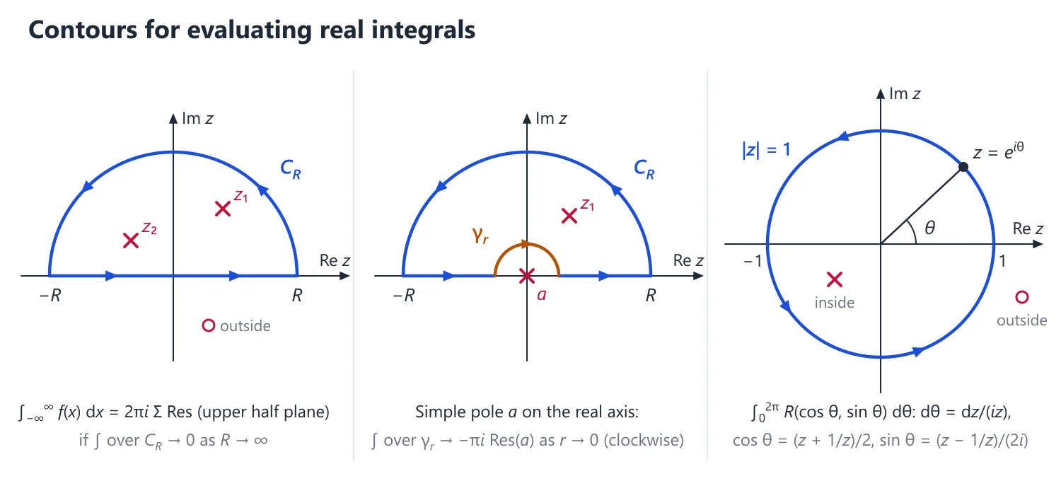
1. Understanding the Unit-Circle Substitution
Why we need it: integrals such as ∫02π dθ/(2 + cos θ) can be done by real methods (the t = tan(θ/2) substitution), but the algebra is heavy and breaks down for squared denominators or numerators like cos 3θ. Turning them into closed contour integrals makes them a residue calculation.
In words: as θ runs from 0 to 2π, the point z = eiθ runs once anticlockwise round the unit circle. Every cos θ, sin θ and dθ can be written in z: cos θ = (z + 1/z)/2, sin θ = (z − 1/z)/(2i), dθ = dz/(iz). The real integral over a full period becomes ∮|z|=1 of a rational function of z.
First example, slowly: I = ∫02π dθ/(2 + cos θ).
(1) Substitute: 2 + cos θ = 2 + (z + 1/z)/2 = (z2 + 4z + 1)/(2z).
(2) Assemble the integrand: (2z/(z2 + 4z + 1))·(1/(iz)) dz = (2/i) dz/(z2 + 4z + 1).
(3) Find the poles: z2 + 4z + 1 = 0 gives α = −2 + √3 ≈ −0.268 and β = −2 − √3 ≈ −3.732. Their product is 1, so exactly one is inside: α.
(4) Residue at the simple pole α: 1/(α − β) = 1/(2√3).
(5) Residue theorem: I = (2/i)·2πi·1/(2√3) = 2π/√3 ≈ 3.628.
(6) Check with the standard result 2π/√(a2 − b2) for a = 2, b = 1: 2π/√3. Notice that the answer is real and positive, as an integral of a positive function must be; an imaginary answer signals a lost factor i.
Non-example: ∫02π dθ/(1 + cos θ). Here a = b = 1, so the condition a > |b| fails: the denominator vanishes at θ = π, the transformed integrand has a pole at z = −1 on the unit circle, and the real integral diverges (near θ = π the integrand behaves like 2/(θ − π)2).
Building up: (i) The substitution needs a full period; for ∫0π of a function of cos θ use symmetry to double the range first. (ii) Only poles strictly inside |z| = 1 count; for a reciprocal pair, check |α| < 1 using αβ = 1. (iii) For numerators cos nθ use Re zn to avoid a high-order pole at 0.
Where it is used: Type I questions, usually 15–20 marks, including ∫ dθ/(a + b cos θ)2 and ∫ sin2θ/(a + b cos θ) dθ.
2. Type I: ∫02π F(cos θ, sin θ) dθ
Substitution: z = eiθ, so cos θ = (z + 1/z)/2, sin θ = (z − 1/z)/(2i), dθ = dz/(iz), and θ from 0 to 2π traces |z| = 1 once anticlockwise.
Why it works: dz = ieiθ dθ = iz dθ, and cos θ = (eiθ + e−iθ)/2 = (z + z−1)/2; more generally cos nθ = (zn + z−n)/2 and sin nθ = (zn − z−n)/(2i). The real integral over one period becomes a closed contour integral of a rational function of z (see the right-hand panel of the figure above).
Condition: F must be continuous on the circle, i.e. its denominator must not vanish for real θ; for a + b cos θ this means a > |b|. Otherwise a pole lies on |z| = 1 and the real integral diverges.
Result: the integral equals 2πi × (sum of residues of the transformed rational function inside |z| = 1).
Derivation of the standard result: for a > |b| > 0, ∫02π dθ/(a + b cos θ) = ∮|z|=1 dz/(iz(a + b(z + 1/z)/2)) = ∮|z|=1 2 dz/(i(bz2 + 2az + b)).
The roots α = (−a + √(a2 − b2))/b and β = (−a − √(a2 − b2))/b are real with αβ = 1 and |α| = (a − √(a2 − b2))/|b| < 1, so only α lies inside the circle.
Res at α = 2/(ib(α − β)) = 2/(i·2√(a2 − b2)), since α − β = 2√(a2 − b2)/b. Hence the integral is 2πi/(i√(a2 − b2)) = 2π/√(a2 − b2); for b = 0 it is simply 2π/a.
Idea: denominators of this type have reciprocal pairs of roots (product 1), so exactly one root of each pair is inside the unit circle; checking |α| < 1 with αβ = 1 saves computing both moduli.
Example 1: Evaluate ∫02π dθ/(5 + 4cos θ).
The integral becomes ∮|z|=1 dz/(iz(5 + 2z + 2/z)) = ∮ dz/(i(2z2 + 5z + 2)) = ∮ dz/(i(2z + 1)(z + 2)). Only z = −1/2 lies inside, with residue 1/(i·2·(−1/2 + 2)) = 1/(3i). The integral is 2πi/(3i) = 2π/3.
General result: ∫02π dθ/(a + b cos θ) = 2π/√(a2 − b2) for a > |b|.
3. Understanding the Semicircle Contour
Why we need it: an integral over the whole real line, such as ∫−∞∞ dx/(x2 + 4), is not over a closed curve, so the residue theorem cannot be applied directly. We close the path with an arc on which the integral becomes negligible.
In words: for a large R, the segment [−R, R] followed by the upper semicircle ΓR: |z| = R, Im z ≥ 0, is a closed anticlockwise contour. It encloses exactly the poles in the upper half-plane with modulus less than R. As R → ∞ the segment integral tends to the real integral, and the arc integral tends to 0 when the degree of the denominator exceeds that of the numerator by at least 2.
First example, slowly: ∫−∞∞ dx/(x2 + 4).
(1) Poles of f(z) = 1/(z2 + 4): z = ±2i. Only 2i is in the upper half-plane.
(2) Residue at 2i: 1/(2z) at z = 2i, i.e. 1/(4i).
(3) For R > 2: ∫−RR f dx + ∫ΓR f dz = 2πi/(4i) = π/2.
(4) Estimate the arc: on |z| = R, |z2 + 4| ≥ R2 − 4, and the arc has length πR, so |∫ΓR f dz| ≤ πR/(R2 − 4) → 0.
(5) Let R → ∞: ∫−∞∞ dx/(x2 + 4) = π/2. Check by real calculus: [(1/2) tan−1(x/2)] from −∞ to ∞ is π/2. Notice that the estimate in step (4) is the part examiners mark; write it every time.
Non-example: ∫−∞∞ x dx/(x2 + 1): the degrees differ by only 1. On the arc f ≈ 1/z, and ∫ΓR dz/z = πi does not tend to 0; correspondingly the real integral diverges (its antiderivative (1/2) ln(x2 + 1) is unbounded), and only the principal value 0 exists.
Building up: (i) deg Q ≥ deg P + 2 gives |f| ≤ K/R2 on the arc, so the ML bound is πK/R → 0. (ii) Closing in the lower half-plane gives the same value with −2πi and the lower poles. (iii) For an even integrand, ∫0∞ is half of ∫−∞∞; for one that is not even, a sector contour may be used instead.
Where it is used: Type II integrals such as ∫ dx/(x2 + a2)2 and ∫ x2 dx/((x2 + 1)(x2 + 4)); the same contour, with Jordan's lemma, handles the Fourier-type integrals.
4. Type II: ∫−∞∞ P(x)/Q(x) dx
Conditions: P, Q polynomials, deg Q ≥ deg P + 2, and Q has no real zeros.
Idea: deg Q ≥ deg P + 2 makes |f(z)| ≤ K/R2 on the arc while the arc length is only πR, so the arc contributes at most πK/R → 0; the same condition makes the real integral converge absolutely. With deg Q = deg P + 1, as for x/(x2 + 1), the improper integral diverges and only a principal value exists. A real zero of Q puts a non-integrable singularity on the path.
Contour: the segment [−R, R] together with the upper semicircle ΓR: |z| = R, Im z ≥ 0. Since |zf(z)| → 0 as |z| → ∞, the ML-inequality gives |∫ΓR f dz| ≤ πR·max|f| → 0.
Result: ∫−∞∞ P(x)/Q(x) dx = 2πi × (sum of residues of P/Q in the upper half-plane).
Why only the upper half-plane: the closed contour (left panel of the figure above) encloses exactly the poles with Im z > 0. One may instead close in the lower half-plane; that contour is clockwise, giving −2πi × (sum of lower residues), the same value. For an even integrand, ∫0∞ = (1/2)∫−∞∞.
Example 2: Evaluate ∫−∞∞ dx/(x2 + 1)2.
The only pole in the upper half-plane is z = i, of order 2. Res = d/dz [(z + i)−2] at z = i = −2/(2i)3 = −2/(−8i) = 1/(4i). The integral is 2πi·1/(4i) = π/2.
Example 3: Evaluate ∫0∞ dx/(x4 + 1).
The poles in the upper half-plane are z1 = eiπ/4 and z2 = e3iπ/4, with residues 1/(4zk3) = −zk/4 (since zk4 = −1). Their sum is −(z1 + z2)/4 = −i√2/4, so ∫−∞∞ = 2πi(−i√2/4) = π/√2 and ∫0∞ = π/(2√2).
5. Understanding Jordan's Lemma and the Factor eimz
Why we need it: integrals with cos mx or sin mx, such as ∫ x sin x/(x2 + 1) dx, often have degrees differing by only 1, so the plain ML estimate fails. And cos mz itself grows exponentially off the real axis. We need a better factor and a better estimate.
In words: for z = x + iy, |eimz| = e−my, which is at most 1 in the upper half-plane when m > 0 and very small high up. Jordan's lemma: if max |f| on the arc ΓR tends to 0, then ∫ΓR eimzf(z) dz → 0. So f only has to tend to 0, not like 1/R2.
First example, slowly: ∫−∞∞ cos 2x/(x2 + 2x + 2) dx and the matching sine integral.
(1) Choose f(z) = e2iz/(z2 + 2z + 2); on the real axis its real part is the cosine integrand and its imaginary part the sine integrand.
(2) Poles: z2 + 2z + 2 = 0 gives z = −1 ± i; only −1 + i is in the upper half-plane.
(3) Residue: e2iz/(2z + 2) at z = −1 + i equals e2i(−1+i)/(2i) = e−2e−2i/(2i).
(4) The arc contribution tends to 0 (here even ML suffices, since the degrees differ by 2 and |e2iz| ≤ 1).
(5) So ∫−∞∞ e2ix/(x2 + 2x + 2) dx = 2πi·e−2e−2i/(2i) = πe−2(cos 2 − i sin 2).
(6) Equate parts: the cosine integral is πe−2 cos 2 ≈ −0.177 and the sine integral is −πe−2 sin 2 ≈ −0.387. Notice that the sine integral is not 0 here because the integrand is not odd: the poles are not symmetric about the imaginary axis.
Non-example: using f(z) = cos 2z/(z2 + 2z + 2) instead. At the top of the arc, z = iR, cos(2iR) = cosh 2R, which grows like e2R/2, so the arc integral does not tend to 0 and the method collapses. The condition that fails is boundedness of the oscillating factor in the upper half-plane.
Building up: (i) On the arc |eimz| = e−mR sin θ. (ii) Jordan's inequality sin θ ≥ 2θ/π on [0, π/2] gives ∫0π e−mR sin θ dθ < π/(mR). (iii) Hence |∫ΓR eimzf dz| < (π/m)·max|f| → 0 (Standard Proofs, Theorem 15). (iv) For m < 0 close in the lower half-plane, or rewrite with −m.
Where it is used: ∫ cos mx/(x2 + a2) dx, ∫ x sin mx/(x2 + a2) dx and similar Fourier-type integrals, and together with indentation for ∫ sin x/x dx.
6. Type III: Fourier-type Integrals and Jordan's Lemma
Jordan's inequality: 2θ/π ≤ sin θ ≤ θ for 0 ≤ θ ≤ π/2.
Why it works: sin θ is concave on [0, π/2], so its graph lies above the chord joining (0, 0) to (π/2, 1), which is the line 2θ/π; and sin θ ≤ θ because the derivative cos θ ≤ 1.
Jordan's lemma: if f(z) → 0 uniformly as |z| → ∞ in the upper half-plane and m > 0, then ∫ΓR eimzf(z) dz → 0 as R → ∞.
Idea: on the arc z = Reiθ, |eimz| = e−mR sin θ, which is tiny except near θ = 0 and θ = π. Jordan's inequality gives ∫0π e−mR sin θ dθ < π/(mR), so |∫ΓR eimzf dz| < (π/m)·maxΓR|f| → 0 (Standard Proofs, Section 15). This is why f → 0 is enough here, whereas the plain ML-inequality needs |f| ≤ K/R2.
If m < 0: eimz grows in the upper half-plane, so close the contour in the lower half-plane (clockwise), or use cos(−mx) = cos mx and sin(−mx) = −sin mx to make m positive.
Method: for ∫−∞∞ f(x) cos mx dx or ∫ f(x) sin mx dx with f = P/Q, deg Q ≥ deg P + 1 and no real poles, integrate eimzf(z) over the semicircle contour and take real or imaginary parts. Never use cos mz directly, since it grows like em|y|.
Why eimz: for real x, cos mx = Re eimx and sin mx = Im eimx (when f is real on ℝ), while |eimz| = e−my ≤ 1 for y ≥ 0. By contrast cos mz = (eimz + e−imz)/2 contains e−imz, whose modulus emy blows up in the upper half-plane.
Example 4: Show that ∫0∞ cos mx/(x2 + a2) dx = (π/(2a))e−ma, for m ≥ 0, a > 0.
Take f(z) = eimz/(z2 + a2). The pole ia is inside, with residue e−ma/(2ia). So ∫−∞∞ eimx/(x2 + a2) dx = 2πi·e−ma/(2ia) = πe−ma/a. Taking real parts and using evenness gives the result.
7. Understanding Indentation and Principal Values
Why we need it: for ∫ sin x/x dx the natural choice eiz/z has a pole at 0, on the path of integration. The residue theorem forbids poles on the contour, so we must step round the pole and keep track of what the detour contributes.
In words: the principal value PV∫−∞∞ f dx is the limit of the integral over the real line with a small symmetric gap (x0 − ε, x0 + ε) removed, as ε → 0. The gap is bridged by a small upper semicircle of radius ε, traversed clockwise; for a simple pole its contribution tends to −πi times the residue there, half of a full circle.
First example, slowly: PV∫−∞∞ dx/((x − 1)(x2 + 1)).
(1) Poles of f(z) = 1/((z − 1)(z2 + 1)): z = 1 on the real axis (simple), z = i above, z = −i below.
(2) Residue at 1: 1/(1 + 1) = 1/2. Residue at i: 1/((i − 1)(2i)) = 1/(−2 − 2i) = −(1 − i)/4.
(3) Contour: [−R, 1 − ε], the small clockwise semicircle round 1, [1 + ε, R], and the large arc (which contributes 0 in the limit since the degrees differ by 3).
(4) The contour encloses only i, so PV∫ − πi·(1/2) = 2πi·(−(1 − i)/4).
(5) Solve: PV∫ = −πi(1 − i)/2 + πi/2 = −πi/2 − π/2 + πi/2 = −π/2. Notice that the imaginary parts cancel, as they must for a real integrand; the PV rule 2πi∑Res(upper) + πi∑Res(real axis) is exactly steps (4) and (5).
Non-example: PV∫−11 dx/x2 does not exist: near 0 the two sides both give +1/ε, which grows without limit, and the small semicircle round a double pole contributes −2c/ε, which also blows up. Indentation works only for simple poles.
Building up: (i) Near a simple pole x0, f = c/(z − x0) + g with g analytic. (ii) On the semicircle z = x0 + εeiθ, θ from π to 0, the c-term gives exactly −πic, and the g-term is at most πε·max|g| → 0. (iii) If the real integrand is finite at x0 (as sin x/x is at 0), the principal value is an ordinary integral and the PV label can be dropped at the end.
Where it is used: ∫0∞ sin x/x dx = π/2, ∫ sin x/(x(x2 + a2)) dx and other integrals whose complex form has a simple pole on the real axis.
8. Poles on the Real Axis and Branch Points
Indentation: if f has a simple pole at a real point x0, avoid it by a small upper semicircle γε of radius ε; as ε → 0, ∫γε f dz → −πi·Res(f, x0) when γε is traversed clockwise.
Derivation: near x0, f(z) = c/(z − x0) + g(z) with c = Res(f, x0) and g analytic. On γε put z = x0 + εeiθ, θ from π to 0 (clockwise, as in the middle panel of the figure above): ∫ c·iεeiθ dθ/(εeiθ) = ic(0 − π) = −πic. The part ∫γε g dz → 0, since g is bounded and the length πε → 0.
Only simple poles: a term c2/(z − x0)2 contributes −2c2/ε over the small semicircle, which blows up; correspondingly the real integral does not exist even as a principal value.
Principal value result: PV∫−∞∞ f dx = 2πi∑Res(upper half-plane) + πi∑Res(simple poles on the real axis).
Idea: a simple pole on the real axis counts half: the small semicircle is half of a full circle round the pole, so it picks up half of 2πi Res.
Example 5: Show that ∫0∞ (sin x)/x dx = π/2.
Take f(z) = eiz/z, with a simple pole at 0 on the contour and no poles above. Indenting at 0 and using Jordan's lemma on the big arc, PV∫−∞∞ eix/x dx = πi·Res(f, 0) = πi. Imaginary parts give ∫−∞∞ (sin x)/x dx = π, and by evenness ∫0∞ = π/2.
Branch points (keyhole contour): for integrals such as ∫0∞ xa−1/(1 + x) dx (0 < a < 1), use a contour that goes around the branch cut along the positive real axis; the result is π/sin(aπ).
Presentation steps:
1. Choose f(z) and the contour, and draw it.
2. Locate the singularities and decide which lie inside.
3. Compute the residues.
4. Show that the integrals over the large arc (ML or Jordan) and small indentations behave as claimed.
5. Let R → ∞ and ε → 0, then equate real or imaginary parts.
9. Choosing the Contour
If the integrand is a rational function of cos θ and sin θ over a full period → unit circle; over [0, π], first check that the integrand is even in θ (a function of cos θ only) and double the range.
If ∫−∞∞ P/Q dx with deg Q − deg P ≥ 2 and no real zeros of Q → large semicircle, arc killed by the ML-inequality.
If there is a factor cos mx or sin mx and deg Q − deg P = 1 → eimz and Jordan's lemma; with deg Q − deg P ≥ 2 the ML-inequality is also enough, because |eimz| ≤ 1.
If the real integrand is finite at a point x0 but eimzf(z) has a simple pole there (as for (sin x)/x) → indented semicircle and the πi Res rule.
If ∫0∞ of a rational function that is not even, such as 1/(1 + x3) → a sector contour of angle 2π/3: on the ray z = re2πi/3, z3 = r3, so (1 − e2πi/3)I = 2πi Res(eiπ/3) = 2πi/(3e2πi/3), giving I = 2π/(3√3).
If xa−1 (0 < a < 1) or log x appears → keyhole contour round a branch cut along the positive real axis, keeping track of the value of arg z on the two edges of the cut.
If parameters appear (a > 0, m > 0, |b| < a) → use them to decide which poles are inside, and state them in the answer.
10. Common Mistakes
1. Integrating cos mz or sin mz over the semicircle instead of eimz; they grow like em|y| and the arc integral does not vanish.
2. Taking the wrong poles: lower half-plane poles in Type II, or both roots of a reciprocal pair in Type I.
3. Forgetting the factor 1/(iz) from dθ = dz/(iz), or the 2i in sin θ = (z − 1/z)/(2i).
4. Asserting that the arc integral tends to 0 without a bound; write the ML estimate (or Jordan's lemma) explicitly, since examiners award marks for it.
5. Using 2πi Res instead of πi Res for a simple pole on the real axis, or indenting round a double pole.
6. Forgetting to halve when ∫0∞ of an even function is obtained from ∫−∞∞, or taking real parts when f is not real on the real axis.
Link: Type III integrals are Fourier transforms, and the inverse Laplace transform is evaluated by the same residue technique on a vertical line closed by a large arc (Ordinary Differential Equations, Laplace transforms).
Link: ∫0∞ (sin x)/x dx = π/2 is also obtained in Real Analysis by differentiating ∫0∞ e−ax(sin x)/x dx with respect to the parameter a; the contour method avoids justifying the interchange of limits.
11. Worked Examples
Example 6: Evaluate ∫02π cos 2θ/(5 − 4 cos θ) dθ.
Consider I = ∫02π e2iθ/(5 − 4 cos θ) dθ; the required integral is Re I. With z = eiθ, 5 − 4 cos θ = 5 − 2(z + 1/z) = −(2z − 1)(z − 2)/z.
So I = ∮|z|=1 z2·(−z/((2z − 1)(z − 2)))·dz/(iz) = i∮|z|=1 z2/((2z − 1)(z − 2)) dz.
Only z = 1/2 lies inside, with residue (1/4)/(2(1/2 − 2)) = −1/12.
I = i·2πi·(−1/12) = π/6, which is real. Hence ∫02π cos 2θ/(5 − 4 cos θ) dθ = π/6 (and the corresponding sine integral is 0).
Example 7: Evaluate ∫−∞∞ x2/((x2 + 1)(x2 + 4)) dx.
deg Q − deg P = 2 and Q has no real zeros, so the integral is 2πi × (sum of residues in the upper half-plane), where the poles are i and 2i (both simple).
Res at i: z2/((z + i)(z2 + 4)) at z = i equals −1/(2i·3) = −1/(6i).
Res at 2i: z2/((z2 + 1)(z + 2i)) at z = 2i equals −4/((−3)(4i)) = 1/(3i).
The integral is 2πi(−1/(6i) + 1/(3i)) = 2π/6 = π/3.
12. Type I Refinements: Half Ranges, Squared Denominators, Parameters
Half range: if the integrand depends on θ only through cos θ, then ∫0π = (1/2)∫02π (substitute θ → 2π − θ), and the full-range integral is done with z = eiθ.
Standard results (a > |b|): ∫02π dθ/(a + b cos θ) = ∫02π dθ/(a + b sin θ) = 2π/√(a2 − b2), and ∫02π dθ/(a + b cos θ)2 = 2πa/(a2 − b2)3/2.
Squared denominator: the transformed integrand has a double pole at the root α inside |z| = 1; use the order-2 formula d/dz[(z − α)2F(z)] at z = α, and simplify with αβ = 1 for the pair of reciprocal roots.
Numerators sin2θ, cos nθ: either write sin2θ = −(z − 1/z)2/4, which creates a pole at z = 0 that must be included, or use cos nθ = Re einθ = Re zn, which avoids that pole.
Real pole together with complex poles: for ∫ R(x) sin mx dx where R(z)eimz has a simple pole at x = 0, use PV∫ = 2πi∑Res(upper half-plane) + πi Res(0) and take imaginary parts.
13. Past UPSC Questions Solved
Example 8 (UPSC 2014, 20 marks): Evaluate the integral ∫0π dθ/(1 + (1/2) cos θ)2 using residues.
(1 + (1/2)cos θ)2 = (2 + cos θ)2/4 and the integrand depends only on cos θ, so I = 4∫0π dθ/(2 + cos θ)2 = 2∫02π dθ/(2 + cos θ)2.
With z = eiθ: 2 + cos θ = (z2 + 4z + 1)/(2z) and dθ = dz/(iz), so ∫02π dθ/(2 + cos θ)2 = ∮|z|=1 4z2/(z2 + 4z + 1)2·dz/(iz) = (4/i)∮ z dz/(z2 + 4z + 1)2.
z2 + 4z + 1 = (z − α)(z − β) with α = −2 + √3 (|α| ≈ 0.27, inside) and β = −2 − √3 (outside); α is a double pole.
Res at α = d/dz[z/(z − β)2] at z = α = −(α + β)/(α − β)3 = 4/(2√3)3 = 1/(6√3).
So ∫02π dθ/(2 + cos θ)2 = (4/i)·2πi/(6√3) = 4π/(3√3), agreeing with 2πa/(a2 − b2)3/2 for a = 2, b = 1; hence I = 8π/(3√3).
Answer: ∫0π dθ/(1 + (1/2)cos θ)2 = 8π/(3√3) = 8√3π/9 ≈ 4.837.
Example 9 (UPSC 2026, 20 marks): Use the method of contour integration to prove ∫02π sin2θ/(a + b cos θ) dθ = (2π/b2){a − √(a2 − b2)}, if a > b > 0.
With z = eiθ: sin2θ = −(z2 − 1)2/(4z2), a + b cos θ = (bz2 + 2az + b)/(2z), dθ = dz/(iz).
So I = −(1/(2ib))∮|z|=1 (z2 − 1)2/(z2(z − α)(z − β)) dz, where α, β = (−a ± √(a2 − b2))/b are the roots of bz2 + 2az + b.
αβ = 1 and |α| = (a − √(a2 − b2))/b = b/(a + √(a2 − b2)) < 1, so α is inside and β outside; z = 0 is a double pole inside.
Res at 0: (z2 − 1)2/(z2 + (2a/b)z + 1) = (1 − 2z2 + ...)(1 − (2a/b)z + ...), whose z-coefficient −2a/b is the residue. Res at α: (α2 − 1)2/(α2(α − β)); since α2 − 1 = α2 − αβ = α(α − β), this equals α − β = 2√(a2 − b2)/b.
I = −(1/(2ib))·2πi·(−2a/b + 2√(a2 − b2)/b) = (2π/b2)(a − √(a2 − b2)).
Answer: ∫02π sin2θ/(a + b cos θ) dθ = (2π/b2){a − √(a2 − b2)}, as required.
Example 10 (UPSC 2021, 20 marks): Using contour integration, evaluate the integral ∫−∞∞ sin x dx/(x(x2 + a2)), a > 0.
Take f(z) = eiz/(z(z2 + a2)), whose imaginary part on the real axis is the integrand. Poles: 0 (on the real axis, simple), ia (upper half-plane), −ia.
Contour: [−R, −ε], the small upper semicircle γε (clockwise), [ε, R] and the large semicircle ΓR. On ΓR, |1/(z(z2 + a2))| ≤ 1/(R(R2 − a2)) → 0, so by Jordan's lemma ∫ΓR f dz → 0, while ∫γε f dz → −πi·Res(f, 0).
Res(f, 0) = 1/a2 and Res(f, ia) = e−a/(ia·2ia) = −e−a/(2a2).
Letting ε → 0, R → ∞: PV∫−∞∞ eix dx/(x(x2 + a2)) = 2πi(−e−a/(2a2)) + πi/a2 = πi(1 − e−a)/a2.
Equate imaginary parts; sin x/(x(x2 + a2)) is continuous at 0, so no principal value is needed for it.
Answer: ∫−∞∞ sin x dx/(x(x2 + a2)) = π(1 − e−a)/a2.
14. Practice Exercises
Exercise 1 (basic): Evaluate ∫02π dθ/(5 + 3 cos θ).
Answer: 2π/√(25 − 9) = π/2.
Exercise 2 (basic): Evaluate ∫−∞∞ dx/(x2 + 9) by residues.
Answer: 2πi·1/(6i) = π/3.
Exercise 3 (basic): Evaluate ∫02π dθ/(3 − 2 sin θ).
Answer: 2π/√(9 − 4) = 2π/√5.
Exercise 4 (standard): Evaluate ∫−∞∞ dx/((x2 + 1)(x2 + 9)).
Answer: residues 1/(16i) at i and −1/(48i) at 3i; 2πi·1/(24i) = π/12.
Exercise 5 (standard): Evaluate ∫0∞ dx/(x2 + 1)3.
Answer: pole of order 3 at i with residue (1/2)·d2/dz2(z + i)−3 at i = 3/(16i); the full-line integral is 3π/8, so the answer is 3π/16.
Exercise 6 (standard): Evaluate ∫0∞ cos 3x/(x2 + 4) dx.
Answer: with e3iz/(z2 + 4), the residue at 2i is e−6/(4i); the full-line integral is πe−6/2, so the answer is (π/4)e−6.
Exercise 7 (standard): Evaluate ∫02π cos 3θ/(5 − 4 cos θ) dθ.
Answer: take Re of ∮ z3·(−z/((2z − 1)(z − 2)))·dz/(iz); the only pole inside is 1/2, giving π/12.
Exercise 8 (UPSC level): Evaluate ∫−∞∞ cos x/(x2 + 1)2 dx, justifying the vanishing of the arc integral.
Answer: f = eiz/(z2 + 1)2, double pole at i with residue d/dz[eiz/(z + i)2] at i = −i/(2e); the integral is 2πi(−i/(2e)) = π/e. The arc bound is πR/(R2 − 1)2 → 0.
Exercise 9 (UPSC level): Evaluate ∫0∞ dx/(1 + x6).
Answer: upper poles eiπ/6, i, e5iπ/6, each with residue −zk/6; their sum is −2i/6, so the full-line integral is 2πi(−i/3) = 2π/3 and the answer is π/3.
Exercise 10 (UPSC level): Show that ∫−∞∞ x sin πx/(x2 + 2x + 5) dx = −πe−2π.
Answer: f = zeiπz/(z2 + 2z + 5), upper pole −1 + 2i with residue (1 − 2i)e−2π/(4i); Jordan's lemma (degrees differ by 1) gives the full integral (π/2)(1 − 2i)e−2π, whose imaginary part is −πe−2π (and the cosine integral is (π/2)e−2π).
| Integral | f(z) and contour | Condition | Key step |
|---|---|---|---|
| ∫02π F(cos θ, sin θ) dθ | z = eiθ, unit circle | F rational, no poles on |z| = 1 | residues inside |z| = 1 |
| ∫−∞∞ P/Q dx | P/Q, upper semicircle | deg Q ≥ deg P + 2, no real zeros of Q | arc → 0 by ML |
| ∫−∞∞ (P/Q) cos mx dx | eimzP/Q, upper semicircle | deg Q ≥ deg P + 1, m > 0 | arc → 0 by Jordan's lemma |
| ∫ with real simple poles | indented semicircle | simple poles on ℝ | small arc → −πi Res |
| ∫0∞ xa−1R(x) dx | keyhole contour | branch cut along [0, ∞) | factor (1 − e2πia) |
Mains points
- Contour integration is asked in almost every paper as a 15 to 20 mark question; the commonest forms are ∫02π dθ/(a + b cos θ), ∫ dx/(x2 + a2)2, ∫ cos mx/(x2 + a2) dx and ∫ (sin x)/x dx.
- Marks are awarded for justifying that the arc integral tends to 0; write the ML or Jordan estimate explicitly rather than simply asserting it.
- For Type I integrals, simplify the denominator into factors and check carefully which root lies inside |z| = 1 (their product is 1 when the polynomial is reciprocal).
- Use eimz, not cos mz or sin mz, and take real or imaginary parts at the end; using cos mz is a frequent error.
- Draw the contour with the poles and the indentations marked, and state the orientation; this makes the solution easy to follow and earns presentation marks.
Did you know?
- The Dirichlet integral ∫0∞ (sin x)/x dx = π/2 is not absolutely convergent, yet contour integration evaluates it in a few lines; real-variable proofs need differentiation under the integral sign or double integrals.
Standard Proofs: Complex Analysis
Seventeen theorems of complex analysis that UPSC asks to be proved: the Cauchy-Riemann conditions, Cauchy's theorem and integral formula, Cauchy's inequality, Liouville and the fundamental theorem of algebra, Morera, Taylor, Riemann's removable singularity theorem, the residue theorem, the maximum modulus principle and Jordan's lemma. The proofs build on each other in the order given.
1. Cauchy-Riemann Equations: Necessary Condition
Statement: Let f = u + iv be defined in a neighbourhood of z0 = x0 + iy0 and differentiable at z0. Then ux, uy, vx, vy exist at (x0, y0), ux = vy and uy = −vx there, and f′(z0) = ux + ivx.
Proof: f′(z0) = limh→0 (f(z0 + h) − f(z0))/h exists, so the limit is the same along every path h → 0.
Take h real: the quotient is [u(x0 + h, y0) − u(x0, y0)]/h + i[v(x0 + h, y0) − v(x0, y0)]/h. A complex limit exists iff the real and imaginary parts converge, so ux, vx exist and f′(z0) = ux + ivx.
Take h = ik with k real: the quotient is [u(x0, y0 + k) − u(x0, y0)]/(ik) + [v(x0, y0 + k) − v(x0, y0)]/k, so uy, vy exist and f′(z0) = vy − iuy.
Equating real and imaginary parts of the two expressions for f′(z0): ux = vy and vx = −uy.
Hence proved.
2. Cauchy-Riemann Equations: Sufficient Condition
Statement: Let u, v have continuous first partial derivatives in a neighbourhood of (x0, y0) and satisfy ux = vy, uy = −vx at (x0, y0). Then f = u + iv is differentiable at z0 and f′(z0) = ux + ivx. If these hold at every point of a domain, f is analytic there.
Proof: Let h = Δx + iΔy be small and write Δu = u(x0 + Δx, y0 + Δy) − u(x0, y0) = [u(x0 + Δx, y0 + Δy) − u(x0, y0 + Δy)] + [u(x0, y0 + Δy) − u(x0, y0)].
By the mean value theorem this equals ux(x0 + θ1Δx, y0 + Δy)Δx + uy(x0, y0 + θ2Δy)Δy with 0 < θ1, θ2 < 1.
By continuity of the partials, Δu = uxΔx + uyΔy + η1Δx + η2Δy with η1, η2 → 0 as h → 0 (partials now taken at (x0, y0)). Similarly Δv = vxΔx + vyΔy + η3Δx + η4Δy.
So Δf = (ux + ivx)Δx + (uy + ivy)Δy + E, where |E| ≤ (|η1| + |η2| + |η3| + |η4|)|h|.
By C-R, uy + ivy = −vx + iux = i(ux + ivx), so Δf = (ux + ivx)(Δx + iΔy) + E = (ux + ivx)h + E.
Therefore |Δf/h − (ux + ivx)| = |E|/|h| → 0, i.e. f′(z0) = ux + ivx.
Hence proved.
3. Real and Imaginary Parts of an Analytic Function are Harmonic
Statement: If f = u + iv is analytic in a domain D, then u and v are harmonic in D.
Proof: The derivative of an analytic function is analytic (Cauchy's integral formula for derivatives), so f has derivatives of all orders, and u, v have continuous partial derivatives of all orders in D.
From the C-R equations ux = vy and uy = −vx, differentiate: uxx = vyx and uyy = −vxy.
The mixed partials of v are continuous, so vxy = vyx (Schwarz), and uxx + uyy = 0.
Similarly vxx = −uyx and vyy = uxy, so vxx + vyy = 0. Hence u and v are harmonic.
Hence proved.
4. The Basic Integral and the ML-Inequality
Statement: (i) If |f| ≤ M on a contour C of length L, then |∫C f(z) dz| ≤ ML. (ii) For every integer n, ∮|z−a|=r (z − a)n dz = 2πi if n = −1 and 0 otherwise.
Proof: (i) With C: z = z(t), a ≤ t ≤ b, |∫C f dz| = |∫ab f(z(t))z′(t) dt| ≤ ∫ab |f(z(t))||z′(t)| dt ≤ M∫ab |z′(t)| dt = ML.
(ii) Parametrise the circle as z = a + reiθ, 0 ≤ θ ≤ 2π, so dz = ireiθ dθ.
Then ∮(z − a)n dz = ∫02π rneinθ·ireiθ dθ = irn+1∫02π ei(n+1)θ dθ.
If n = −1 the integrand is 1, giving i·2π = 2πi. If n ≠ −1, ∫02π ei(n+1)θ dθ = [ei(n+1)θ/(i(n + 1))]02π = 0.
Hence proved.
5. Cauchy's Theorem (with Continuous Derivative)
Statement: Let f be analytic, with f′ continuous, inside and on a simple closed contour C. Then ∮C f(z) dz = 0. (Goursat showed that continuity of f′ need not be assumed.)
Proof: Write f = u + iv and dz = dx + i dy. Then ∮C f dz = ∮C (u dx − v dy) + i∮C (v dx + u dy).
Since f′ = ux + ivx = vy − iuy is continuous, u and v have continuous first partials on the closed region R bounded by C, so Green's theorem ∮(P dx + Q dy) = ∬R(Qx − Py) dx dy applies.
First integral (P = u, Q = −v): ∬R(−vx − uy) dx dy = 0, because uy = −vx.
Second integral (P = v, Q = u): ∬R(ux − vy) dx dy = 0, because ux = vy.
Hence ∮C f(z) dz = 0.
Hence proved.
6. Cauchy's Integral Formula
Statement: Let f be analytic inside and on a simple closed contour C, described anticlockwise, and let z0 be a point inside C. Then f(z0) = (1/2πi)∮C f(z)/(z − z0) dz.
Proof: Let Cρ be the circle |z − z0| = ρ, with ρ so small that Cρ lies inside C. The function g(z) = f(z)/(z − z0) is analytic on and between C and Cρ.
By the deformation theorem, ∮C g dz = ∮Cρ g dz for every such ρ.
Write ∮Cρ g dz = f(z0)∮Cρ dz/(z − z0) + ∮Cρ (f(z) − f(z0))/(z − z0) dz = 2πif(z0) + Iρ, using the basic integral.
Let ε > 0. By continuity of f at z0 there is δ > 0 with |f(z) − f(z0)| < ε when |z − z0| < δ. For ρ < δ, the ML-inequality gives |Iρ| ≤ (ε/ρ)·2πρ = 2πε.
So |∮C g dz − 2πif(z0)| ≤ 2πε. The left side does not depend on ε, so it is 0, and f(z0) = (1/2πi)∮C f(z)/(z − z0) dz.
Hence proved.
7. Cauchy's Inequality
Statement: Let f be analytic inside and on the circle C: |z − z0| = r, and let |f(z)| ≤ M on C. Then |f(n)(z0)| ≤ n!M/rn for n = 0, 1, 2, ....
Proof: By Cauchy's integral formula for derivatives, f(n)(z0) = (n!/2πi)∮C f(z)/(z − z0)n+1 dz.
On C, |z − z0| = r, so |f(z)/(z − z0)n+1| ≤ M/rn+1; the length of C is 2πr.
By the ML-inequality, |f(n)(z0)| ≤ (n!/2π)·(M/rn+1)·2πr = n!M/rn.
Hence proved.
8. Liouville's Theorem
Statement: A bounded entire function is constant: if f is analytic on all of ℂ and |f(z)| ≤ M for every z, then f is constant.
Proof: Fix z0 ∈ ℂ. Since f is entire, it is analytic inside and on |z − z0| = R for every R > 0, and |f| ≤ M there.
Cauchy's inequality with n = 1 gives |f′(z0)| ≤ M/R for every R > 0.
Letting R → ∞, f′(z0) = 0. As z0 was arbitrary, f′ ≡ 0 on ℂ.
Then ux = uy = vx = vy = 0 everywhere (f′ = ux + ivx = vy − iuy), so u and v are constant on the connected set ℂ, and f is constant.
Hence proved.
9. Fundamental Theorem of Algebra
Statement: Every polynomial p(z) = anzn + ... + a0 of degree n ≥ 1 with complex coefficients has a zero in ℂ; consequently it has exactly n zeros counted with multiplicity.
Proof: Suppose p(z) ≠ 0 for every z. Then g = 1/p is entire.
p(z) = anzn(1 + an−1/(anz) + ... + a0/(anzn)), and the bracket tends to 1 as |z| → ∞. So there is R with |p(z)| ≥ |an||z|n/2 ≥ |an|Rn/2 for |z| ≥ R.
Thus |g| ≤ 2/(|an|Rn) for |z| ≥ R, and g is bounded on the compact disc |z| ≤ R because it is continuous. So g is a bounded entire function.
By Liouville's theorem g, and hence p, is constant, contradicting n ≥ 1. So p(z1) = 0 for some z1.
Dividing, p(z) = (z − z1)q(z) with deg q = n − 1; repeating the argument (induction on n) gives exactly n zeros counted with multiplicity.
Hence proved.
10. Morera's Theorem
Statement: Let f be continuous in a domain D, and suppose ∮C f(z) dz = 0 for every closed contour C in D. Then f is analytic in D.
Proof: Analyticity is local, so fix an open disc Δ ⊆ D with centre z0. For z ∈ Δ define F(z) = ∫[z0, z] f(ζ) dζ along the line segment, which lies in Δ.
For z, z + h ∈ Δ, the triangle z0 → z → z + h → z0 is a closed contour in Δ, so its integral is 0, which gives F(z + h) − F(z) = ∫[z, z+h] f(ζ) dζ.
Since ∫[z, z+h] dζ = h, (F(z + h) − F(z))/h − f(z) = (1/h)∫[z, z+h] (f(ζ) − f(z)) dζ.
By the ML-inequality its modulus is at most max{|f(ζ) − f(z)| : ζ ∈ [z, z + h]}, which tends to 0 as h → 0 by continuity of f. So F′(z) = f(z) on Δ, and F is analytic in Δ.
The derivative of an analytic function is analytic (Cauchy's formula for derivatives), so f = F′ is analytic in Δ. As Δ was arbitrary, f is analytic in D.
Hence proved.
11. Taylor's Theorem
Statement: If f is analytic in the disc |z − z0| < R, then f(z) = ∑n=0∞ an(z − z0)n for every z in the disc, where an = f(n)(z0)/n!.
Proof: Fix z with |z − z0| < R and choose r with |z − z0| < r < R. Let C be the circle |ζ − z0| = r. By Cauchy's formula, f(z) = (1/2πi)∮C f(ζ)/(ζ − z) dζ.
For ζ on C, 1/(ζ − z) = (1/(ζ − z0))·1/(1 − w) with w = (z − z0)/(ζ − z0) and |w| = |z − z0|/r = q < 1.
Hence 1/(ζ − z) = ∑n=0∞ (z − z0)n/(ζ − z0)n+1, and with M = maxC |f| the n-th term of f(ζ)/(ζ − z) is bounded by Mqn/r on C.
∑Mqn/r converges, so by the M-test the series converges uniformly on C and may be integrated term by term.
This gives f(z) = ∑n=0∞ (z − z0)n·(1/2πi)∮C f(ζ)/(ζ − z0)n+1 dζ = ∑ f(n)(z0)(z − z0)n/n!, by Cauchy's formula for derivatives.
Hence proved.
12. Riemann's Theorem on Removable Singularities
Statement: Let f be analytic in 0 < |z − z0| < r and bounded there. Then z0 is a removable singularity: limz→z0 f(z) exists, and defining f(z0) as this limit makes f analytic at z0.
Proof: By Laurent's theorem f(z) = ∑n=−∞∞ an(z − z0)n in the punctured disc, with a−n = (1/2πi)∮|z−z0|=ρ f(z)(z − z0)n−1 dz for any 0 < ρ < r and n ≥ 1.
Let |f| ≤ M. On the circle |(z − z0)n−1| = ρn−1 and the length is 2πρ, so by the ML-inequality |a−n| ≤ (1/2π)·Mρn−1·2πρ = Mρn.
This holds for every ρ in (0, r); letting ρ → 0 gives a−n = 0 for all n ≥ 1.
So the principal part vanishes and f(z) = ∑n≥0 an(z − z0)n, a power series, for 0 < |z − z0| < r. Setting f(z0) = a0 = limz→z0 f(z) makes f analytic at z0.
Hence proved.
13. Cauchy's Residue Theorem
Statement: Let C be a simple closed contour described anticlockwise, and let f be analytic inside and on C except at finitely many isolated singular points z1, ..., zn inside C. Then ∮C f(z) dz = 2πi ∑k=1n Res(f, zk).
Proof: Around each zk draw a circle Ck: |z − zk| = ρk, so small that the circles lie inside C, do not meet one another, and f is analytic in 0 < |z − zk| ≤ ρk.
f is analytic on the closed region bounded externally by C and internally by C1, ..., Cn. By Cauchy's theorem for multiply connected regions, ∮C f dz = ∑k∮Ck f dz, all circles anticlockwise.
On Ck, f(z) = ∑m=−∞∞ am(k)(z − zk)m (Laurent series), which converges uniformly on the circle, so it can be integrated term by term.
By the basic integral only the term m = −1 survives: ∮Ck f dz = 2πia−1(k) = 2πi Res(f, zk).
Summing over k gives ∮C f dz = 2πi ∑ Res(f, zk).
Hence proved.
14. Maximum Modulus Principle
Statement: Let f be analytic in a domain D. If |f| attains its maximum at a point z0 ∈ D, then f is constant in D.
Proof: Let M = |f(z0)| and choose ρ with the closed disc |z − z0| ≤ ρ in D. For 0 < r ≤ ρ, Cauchy's formula on |z − z0| = r (put z = z0 + reiθ) gives Gauss's mean value f(z0) = (1/2π)∫02π f(z0 + reiθ) dθ.
Hence M ≤ (1/2π)∫02π |f(z0 + reiθ)| dθ ≤ M, so ∫02π (M − |f(z0 + reiθ)|) dθ = 0.
The integrand is continuous and non-negative, so it vanishes identically: |f| = M on every circle |z − z0| = r ≤ ρ, i.e. on the whole disc Δ.
If M = 0, f = 0 on Δ. Otherwise differentiate u2 + v2 = M2: uux + vvx = 0 and uuy + vvy = 0; with C-R these become uux − vuy = 0 and vux + uuy = 0.
Solving, (u2 + v2)ux = 0 and (u2 + v2)uy = 0, so ux = uy = 0, hence vx = vy = 0, and f is constant on Δ.
f equals a constant on the open disc Δ, so by the identity theorem f is that constant throughout the domain D.
Hence proved.
15. Jordan's Lemma
Statement: Let ΓR be the upper semicircle |z| = R, Im z ≥ 0, let f be continuous on ΓR for all large R with M(R) = maxΓR |f| → 0 as R → ∞, and let m > 0. Then ∫ΓR eimzf(z) dz → 0 as R → ∞.
Proof: On ΓR, z = Reiθ (0 ≤ θ ≤ π), dz = iReiθ dθ and |eimz| = |eimR(cos θ + i sin θ)| = e−mR sin θ.
So |∫ΓR eimzf dz| ≤ M(R)R∫0π e−mR sin θ dθ = 2M(R)R∫0π/2 e−mR sin θ dθ, using sin(π − θ) = sin θ.
Jordan's inequality: sin θ ≥ 2θ/π on [0, π/2], because sin is concave there and the chord joins (0, 0) to (π/2, 1).
Hence the bound is at most 2M(R)R∫0π/2 e−2mRθ/π dθ = 2M(R)R·(π/(2mR))(1 − e−mR) < πM(R)/m.
Since M(R) → 0, the integral tends to 0 as R → ∞.
Hence proved.
16. A Power Series is Analytic inside its Circle of Convergence
Statement: Let f(z) = ∑n=0∞ anzn have radius of convergence R > 0. Then f is analytic in |z| < R and f′(z) = ∑n=1∞ nanzn−1 there; repeating, f has derivatives of all orders and an = f(n)(0)/n!.
Proof: Since lim n1/n = 1, the series ∑nanzn−1 and ∑n(n − 1)anzn−2 also have radius R (Cauchy–Hadamard). Let g(z) = ∑nanzn−1.
Fix z with |z| < R and choose r with |z| < r < R. For 0 < |h| < r − |z|: (f(z + h) − f(z))/h − g(z) = ∑n≥2 an[((z + h)n − zn)/h − nzn−1].
By the binomial theorem the bracket is ∑k=2n C(n, k)zn−khk−1, so its modulus is at most |h|∑k=2n C(n, k)|z|n−k|h|k−2.
Since C(n, k) ≤ C(n, 2)C(n − 2, k − 2) for 2 ≤ k ≤ n (their ratio is k(k − 1)/2 ≥ 1), this is at most |h|(n(n − 1)/2)(|z| + |h|)n−2 ≤ |h|(n(n − 1)/2)rn−2.
Hence |(f(z + h) − f(z))/h − g(z)| ≤ (|h|/2)∑n≥2 n(n − 1)|an|rn−2, and this series converges because r < R (absolute convergence inside the radius).
Letting h → 0 the right side tends to 0, so f′(z) = g(z); f is differentiable at every point of |z| < R, i.e. analytic there.
Applying the result to g repeatedly, f(k)(z) = ∑n≥k n(n − 1)...(n − k + 1)anzn−k, and z = 0 gives f(k)(0) = k!ak.
Hence proved.
17. Poles of Order m: Characterisation and Residue Formula
Statement: Let z0 be an isolated singular point of f. Then z0 is a pole of order m (m ≥ 1) if and only if f(z) = φ(z)/(z − z0)m near z0, where φ is analytic at z0 and φ(z0) ≠ 0. In that case Res(f, z0) = φ(m−1)(z0)/(m − 1)!.
Proof: f is analytic in some 0 < |z − z0| < r, so f(z) = ∑n=−∞∞ an(z − z0)n there (Laurent's theorem).
(⇒) A pole of order m means a−m ≠ 0 and an = 0 for n < −m. Then (z − z0)mf(z) = ∑k=0∞ ak−m(z − z0)k for 0 < |z − z0| < r.
This power series converges in the punctured disc, hence in the whole disc |z − z0| < r; its sum φ is analytic there (Proof 16), φ(z0) = a−m ≠ 0, and f = φ/(z − z0)m.
(⇐) If f = φ/(z − z0)m with φ analytic and φ(z0) ≠ 0, expand φ(z) = ∑k=0∞ bk(z − z0)k (Taylor), b0 = φ(z0) ≠ 0.
Then f(z) = ∑k=0∞ bk(z − z0)k−m, which by uniqueness is the Laurent series of f; its principal part is b0/(z − z0)m + ... + bm−1/(z − z0) with b0 ≠ 0, so z0 is a pole of order m.
The residue is the coefficient of (z − z0)−1, namely bm−1 (the term k = m − 1), and by Taylor's theorem bm−1 = φ(m−1)(z0)/(m − 1)!.
Hence proved.
Mains points
- Most frequently asked: the C-R equations (necessary, and sufficient with continuous partials), Cauchy's integral formula, Liouville's theorem with the fundamental theorem of algebra as a corollary, the residue theorem and Jordan's lemma.
- State the hypotheses on the contour precisely: simple closed, positively oriented, f analytic inside and on it, the point z0 inside. Most lost marks come from applying Cauchy's formula when the point is outside or on the contour.
- Present the analysis steps that make these proofs rigorous: the ML-inequality bound with the length written out, the uniform convergence that justifies term-by-term integration (Taylor, residue theorem), and the continuity argument with ε in Cauchy's formula.
- In a 10-mark answer, Liouville, the fundamental theorem of algebra and Cauchy's inequality can be chained in about a page: inequality ⇒ f′ = 0 ⇒ constant ⇒ 1/p bounded ⇒ contradiction.
- Draw the contour (circle, semicircle with the large arc, indentations) in proofs such as Jordan's lemma and the residue theorem; examiners expect the figure.
Did you know?
- Liouville's theorem is named after Joseph Liouville, who lectured on it in 1847, but Cauchy had published it in 1844; the 'Liouville' name stuck through Liouville's students' notes.
Solved Problems: Complex Analysis
Thirteen UPSC-style problems spanning analytic functions and Cauchy's theorem, series and singularities, and residues and contour integration, each worked step by step to a stated answer.
1. Analytic Functions and Cauchy's Theorem
Problem 1 (10 marks): Show that v = e−x(x cos y + y sin y) is harmonic, and find the analytic function f = u + iv with f(0) = 1.
vx = e−x(−x cos y − y sin y + cos y) and vy = e−x(−x sin y + sin y + y cos y).
vxx = e−x(x cos y + y sin y − 2cos y) and vyy = e−x(−x cos y + 2cos y − y sin y), so vxx + vyy = 0: v is harmonic.
Milne-Thomson for given v: f′(z) = vy(z, 0) + ivx(z, 0) = 0 + ie−z(1 − z).
∫(1 − z)e−z dz = ze−z (check: d/dz(ze−z) = (1 − z)e−z), so f(z) = ize−z + C with C real.
f(0) = C = 1. Then u = Re f = e−x(x sin y − y cos y) + 1.
Answer: f(z) = ize−z + 1, with u = e−x(x sin y − y cos y) + 1.
Problem 2 (15 marks): If f = u + iv is analytic and u − v = (x − y)(x2 + 4xy + y2), find f in terms of z.
Consider F = (1 + i)f = (u − v) + i(u + v), which is analytic with real part U = u − v.
Expanding, U = x3 + 3x2y − 3xy2 − y3, so Ux = 3x2 + 6xy − 3y2 and Uy = 3x2 − 6xy − 3y2.
Milne-Thomson: F′(z) = Ux(z, 0) − iUy(z, 0) = 3z2 − 3iz2 = 3(1 − i)z2, so F = (1 − i)z3 + c.
Then f = F/(1 + i) = ((1 − i)/(1 + i))z3 + c′ = −iz3 + c′.
Check: −iz3 = (3x2y − y3) + i(3xy2 − x3), and u − v = x3 + 3x2y − 3xy2 − y3, as required.
Answer: f(z) = −iz3 + c′, where c′ is a complex constant with Re c′ = Im c′ (so that u − v is unchanged).
Problem 3 (10 marks): Evaluate ∫C z̄ dz from 0 to 1 + i along (i) the line y = x, (ii) the parabola y = x2. What do you conclude?
(i) z = t(1 + i), 0 ≤ t ≤ 1, z̄ = t(1 − i), dz = (1 + i) dt. The integral is ∫01 t(1 − i)(1 + i) dt = ∫01 2t dt = 1.
(ii) z = t + it2, z̄ = t − it2, dz = (1 + 2it) dt, and (t − it2)(1 + 2it) = t + it2 + 2t3.
So the integral is ∫01 (t + 2t3) dt + i∫01 t2 dt = 1/2 + 1/2 + i/3 = 1 + i/3.
The values differ, so the integral depends on the path; this is consistent with z̄ not being analytic (C-R fails: ux = 1 ≠ −1 = vy).
Answer: (i) 1, (ii) 1 + i/3; the integral of the non-analytic function z̄ is path-dependent.
Problem 4 (15 marks): Evaluate ∮C (z + 1)/(z3 − 2z2) dz, where C is (i) |z| = 1, (ii) |z − 2 − i| = 2, (iii) |z − 1 − 2i| = 2, each taken anticlockwise.
The integrand is (z + 1)/(z2(z − 2)), singular at z = 0 and z = 2.
(i) Only z = 0 is inside. With g(z) = (z + 1)/(z − 2), the derivative formula gives ∮ g(z)/z2 dz = 2πig′(0). g′(z) = −3/(z − 2)2, g′(0) = −3/4, so the value is −3πi/2.
(ii) |2 − (2 + i)| = 1 < 2, so z = 2 is inside; |0 − (2 + i)| = √5 > 2, so z = 0 is outside. With h(z) = (z + 1)/z2, the value is 2πih(2) = 2πi·3/4 = 3πi/2.
(iii) |0 − (1 + 2i)| = √5 > 2 and |2 − (1 + 2i)| = √5 > 2, so both points are outside; the integrand is analytic inside and on C, and the integral is 0 by Cauchy's theorem.
Answer: (i) −3πi/2, (ii) 3πi/2, (iii) 0.
2. Series and Singularities
Problem 5 (15 marks): Expand f(z) = (7z − 2)/(z(z + 1)(z − 2)) in a Laurent series valid in 1 < |z + 1| < 3.
Partial fractions: f = A/z + B/(z + 1) + C/(z − 2) with A = (−2)/((1)(−2)) = 1, B = (−9)/((−1)(−3)) = −3, C = 12/(2·3) = 2.
Put w = z + 1, so 1 < |w| < 3 and f = 1/(w − 1) − 3/w + 2/(w − 3).
Since |w| > 1: 1/(w − 1) = (1/w)·1/(1 − 1/w) = ∑n=1∞ w−n.
Since |w| < 3: 2/(w − 3) = −(2/3)·1/(1 − w/3) = −∑n=0∞ 2wn/3n+1.
Combining, f = −2/w + ∑n=2∞ w−n − ∑n=0∞ 2wn/3n+1.
Answer: f(z) = ... + 1/(z + 1)3 + 1/(z + 1)2 − 2/(z + 1) − 2/3 − 2(z + 1)/9 − 2(z + 1)2/27 − ..., valid for 1 < |z + 1| < 3.
Problem 6 (10 marks): Find the first three non-zero terms of the Taylor series of tan z about z = 0, and its radius of convergence.
tan z is odd, so write tan z = a1z + a3z3 + a5z5 + ... and use sin z = tan z·cos z.
z − z3/6 + z5/120 − ... = (a1z + a3z3 + a5z5)(1 − z2/2 + z4/24 − ...).
Comparing coefficients: z: a1 = 1; z3: a3 − 1/2 = −1/6, so a3 = 1/3; z5: a5 − a3/2 + 1/24 = 1/120, so a5 = 1/120 + 1/6 − 1/24 = 2/15.
The nearest singularities of tan z to 0 are the poles ±π/2, so the radius of convergence is π/2.
Answer: tan z = z + z3/3 + 2z5/15 + ..., with radius of convergence π/2.
Problem 7 (15 marks): Determine the nature of the singularities and the residues of (i) (ez − 1)/z, (ii) ze1/z, (iii) 1/(z(ez − 1)).
(i) (ez − 1)/z = 1 + z/2! + z2/3! + ... has no negative powers: z = 0 is a removable singularity (limit 1), residue 0.
(ii) ze1/z = z(1 + 1/z + 1/(2!z2) + 1/(3!z3) + ...) = z + 1 + 1/(2z) + 1/(6z2) + ...: infinitely many negative powers, so z = 0 is an essential singularity, with residue 1/2.
(iii) ez − 1 = z(1 + z/2 + z2/6 + ...), so near 0, f = (1/z2)(1 + z/2 + z2/6 + ...)−1 = (1/z2)(1 − z/2 + z2/12 − ...). So z = 0 is a pole of order 2 with residue −1/2.
Also ez = 1 at z = 2nπi (n ≠ 0), where ez − 1 has simple zeros (derivative ez = 1 ≠ 0). These are simple poles, with residue 1/(z·ez) at z = 2nπi, i.e. 1/(2nπi).
Answer: (i) removable at 0, residue 0; (ii) essential at 0, residue 1/2; (iii) pole of order 2 at 0 with residue −1/2, and simple poles at 2nπi (n ≠ 0) with residues 1/(2nπi).
Problem 8 (10 marks): Evaluate ∮|z|=2 dz/(z5 − 1).
The poles are the fifth roots of unity zk = e2πik/5, k = 0, ..., 4, all simple and all inside |z| = 2.
Res(f, zk) = 1/(5zk4) = zk/(5zk5) = zk/5, since zk5 = 1.
The sum of the fifth roots of unity is 0 (they are the roots of z5 − 1, whose z4 coefficient is 0), so the sum of residues is 0.
Equivalently, f = z−5(1 − z−5)−1 has no 1/z term for large |z|, so Res(f, ∞) = 0 and the finite residues add to 0.
Answer: The integral is 0.
3. Residues and Contour Integration
Problem 9 (15 marks): Show that ∫02π dθ/(1 − 2p cos θ + p2) = 2π/(1 − p2) for 0 < p < 1.
Put z = eiθ, cos θ = (z + 1/z)/2, dθ = dz/(iz). Then 1 − 2p cos θ + p2 = (−pz2 + (1 + p2)z − p)/z = (1 − pz)(z − p)/z.
The integral becomes ∮|z|=1 dz/(i(1 − pz)(z − p)).
The poles are z = p (inside, as 0 < p < 1) and z = 1/p (outside).
Res at z = p = 1/(i(1 − p2)). By the residue theorem the integral is 2πi/(i(1 − p2)) = 2π/(1 − p2).
Answer: ∫02π dθ/(1 − 2p cos θ + p2) = 2π/(1 − p2) (and 2π/(p2 − 1) when p > 1, where only z = 1/p lies inside).
Problem 10 (15 marks): Using contour integration, show that ∫−∞∞ x sin x/(x2 + a2) dx = πe−a for a > 0.
Take f(z) = zeiz/(z2 + a2) on the contour [−R, R] plus the upper semicircle ΓR. Never use sin z directly, since it grows in the upper half-plane.
On ΓR, |z/(z2 + a2)| ≤ R/(R2 − a2) → 0, so by Jordan's lemma (m = 1) ∫ΓR f dz → 0.
The only pole in the upper half-plane is z = ia (simple), with residue iae−a/(2ia) = e−a/2.
Letting R → ∞, ∫−∞∞ xeix/(x2 + a2) dx = 2πi·e−a/2 = πie−a.
Equating imaginary parts gives the result (the real part ∫ x cos x/(x2 + a2) dx = 0, as expected for an odd integrand).
Answer: ∫−∞∞ x sin x/(x2 + a2) dx = πe−a.
Problem 11 (15 marks): Evaluate ∫0∞ dx/(1 + x3) by integrating over a suitable sector.
Let I be the integral and f(z) = 1/(1 + z3). Use the sector 0 ≤ arg z ≤ 2π/3, |z| ≤ R: the segment [0, R], the arc |z| = R, and the ray z = re2πi/3 back to 0.
On the ray z3 = r3 and dz = e2πi/3 dr, so that side contributes −e2πi/3∫0R dr/(1 + r3). On the arc |f| ≤ 1/(R3 − 1) and the length is 2πR/3, so by ML that integral → 0.
The only pole inside is z0 = eiπ/3, with residue 1/(3z02) = e−2πi/3/3.
Letting R → ∞: (1 − e2πi/3)I = 2πie−2πi/3/3, i.e. (e2πi/3 − e4πi/3)I = 2πi/3.
e2πi/3 − e4πi/3 = 2i sin(2π/3) = i√3, so I = 2π/(3√3).
Answer: ∫0∞ dx/(1 + x3) = 2π/(3√3) ≈ 1.2092.
Problem 12 (10 marks): Show that all five zeros of z5 + 15z + 1 lie in |z| < 2, and that exactly one of them lies in |z| < 3/2.
On |z| = 2 take f = z5, g = 15z + 1: |g| ≤ 31 < 32 = |f|. By Rouché, z5 + 15z + 1 has 5 zeros in |z| < 2, the same number as z5.
On |z| = 3/2 take f = 15z, g = z5 + 1: |g| ≤ (3/2)5 + 1 = 243/32 + 1 ≈ 8.59 < 22.5 = |f|. So there is exactly one zero in |z| < 3/2.
There are no zeros on |z| = 3/2 (there |p| ≥ 22.5 − 8.59 > 0), so the other four lie in 3/2 < |z| < 2.
Answer: All 5 zeros lie in |z| < 2: one in |z| < 3/2 and four in 3/2 < |z| < 2.
Problem 13 (15 marks): Evaluate ∫−∞∞ cos x/((x2 + 1)(x2 + 4)) dx.
Take f(z) = eiz/((z2 + 1)(z2 + 4)) on the upper semicircular contour. On the arc |f| ≤ 1/((R2 − 1)(R2 − 4)) since |eiz| ≤ 1 for Im z ≥ 0, so by ML the arc integral → 0.
Res at i: e−1/((2i)(3)) = e−1/(6i).
Res at 2i: e−2/((−3)(4i)) = −e−2/(12i).
∫−∞∞ eix/((x2 + 1)(x2 + 4)) dx = 2πi(e−1/(6i) − e−2/(12i)) = π(2e−1 − e−2)/6.
This is real, so it equals the cosine integral (the sine integral is 0 by oddness).
Answer: ∫−∞∞ cos x/((x2 + 1)(x2 + 4)) dx = (π/6)(2/e − 1/e2) ≈ 0.3144.
Mains points
- In every contour problem write four things: the function f(z) chosen, the contour (with a sketch), which singularities lie inside (with the distance check), and why the extra arcs contribute nothing (ML or Jordan).
- For residues, choose the quickest method: p/q′ for simple poles, the order-m derivative formula for low-order poles of simple functions, and Laurent expansion for essential singularities or messy higher-order poles.
- In Milne-Thomson problems, add the correct constant: iC when u is given, a real C when v is given, and use a given value such as f(0) to fix it.
- Rouché questions need the strict inequality |g| < |f| on the whole circle, shown with a numerical bound, and a remark that no zero lies on the circle itself.
Did you know?
- Problem 8 is a quick consistency check worth remembering: when the integrand is a rational function whose denominator degree exceeds the numerator degree by at least 2, the residues at all finite poles add up to 0.
UPSC Previous Year Questions: Complex Analysis
All 45 question parts (640 marks) on Complex Analysis asked in UPSC CSE Mathematics Optional papers from 2014–2026, transcribed from the official papers on upsc.gov.in and grouped by the topic in these notes that teaches them. The most heavily examined areas are Contour Integration: Evaluation of Real Integrals and Analytic Functions and Cauchy-Riemann Equations.
1. Analytic Functions and Cauchy-Riemann Equations
2026 Paper II, Q1(d), 10 marks: Show that the function f(z) = √|xy| is not analytic at the origin, although Cauchy-Riemann equations are satisfied at that point.
2024 Paper II, Q1(b), 10 marks: If w = f(z) is an analytic function of z, then show that (∂2/∂x2 + ∂2/∂y2) log |f′(z)| = 0.
2024 Paper II, Q1(d), 10 marks: If φ and ψ are functions of x and y satisfying Laplace equation, then show that f(z) = p + iq, i = √−1 is an analytic function, where p = ∂φ/∂y − ∂ψ/∂x and q = ∂φ/∂x + ∂ψ/∂y.
2023 Paper II, Q1(d), 10 marks: State the sufficient conditions for a function f(z) = f(x + iy) = u(x, y) + iv(x, y) to be analytic in its domain. Hence, show that f(z) = log z is analytic in its domain and find df/dz.
2023 Paper II, Q3(b), 15 marks: Prove that u(x, y) = ex(x cos y − y sin y) is harmonic. Find its conjugate harmonic function v(x, y) and express the corresponding analytic function f(z) in terms of z.
2022 Paper II, Q1(b), 10 marks: If f(z) = u + iv is an analytic function of z, and u − v = (cos x + sin x − e−y)/(2 cos x − ey − e−y), then find f(z) subject to the condition f(π/2) = 0.
2020 Paper II, Q4(a), 15 marks: If v(r, θ) = (r − 1/r) sin θ, r ≠ 0, then find an analytic function f(z) = u(r, θ) + iv(r, θ)
2019 Paper II, Q1(d), 10 marks: Suppose f(z) is analytic function on a domain D in ℂ and satisfies the equation Im f(z) = (Re f(z))2, z ∈ D. Show that f(z) is constant in D.
2018 Paper II, Q1(c), 10 marks: Prove that the function : u(x, y) = (x − 1)3 − 3xy2 + 3y2 is harmonic and find its harmonic conjugate and the corresponding analytic function f(z) in terms of z.
2017 Paper II, Q3(b), 15 marks: Let f = u + iv be an analytic function on the unit disc D = {z ∈ ℂ : |z| < 1}. Show that
∂2u/∂x2 + ∂2u/∂y2 = 0 = ∂2v/∂x2 + ∂2v/∂y2
at all points of D.
2016 Paper II, Q1(d), 10 marks: Is v(x, y) = x3 − 3xy2 + 2y a harmonic function? Prove your claim. If yes, find its conjugate harmonic function u(x, y) and hence obtain the analytic function whose real and imaginary parts are u and v respectively.
2015 Paper II, Q1(d), 10 marks: Show that the function v(x, y) = ln(x2 + y2) + x + y is harmonic. Find its conjugate harmonic function u(x, y). Also, find the corresponding analytic function f(z) = u + iv in terms of z.
2014 Paper II, Q1(c), 10 marks: Prove that the function f(z) = u + iv, where f(z) = [x3(1 + i) − y3(1 − i)]/(x2 + y2), z ≠ 0; f(0) = 0 satisfies Cauchy-Riemann equations at the origin, but the derivative of f at z = 0 does not exist.
2. Cauchy's Theorem and Cauchy's Integral Formula
2024 Paper II, Q2(c), 20 marks: Find the function which is analytic inside and on the circle C : z = eiθ, 0 ≤ θ ≤ 2π and has the value [(a2 − 1) cos θ + i(a2 + 1) sin θ]/(a4 − 2a2 cos 2θ + 1), on the circumference of C, where a2 > 1.
2022 Paper II, Q3(a), 15 marks: Evaluate ∫C (z + 4)/(z2 + 2z + 5) dz, where C is |z + 1 − i| = 2.
2020 Paper II, Q1(d), 10 marks: Evaluate the integral ∫C (z2 + 3z) dz counterclockwise from (2, 0) to (0, 2) along the curve C, where C is the circle |z| = 2.
2019 Paper II, Q3(c), 10 marks: Evaluate the integral ∫C Re(z2) dz from 0 to 2 + 4i along the curve C where C is a parabola y = x2.
3. Power Series, Taylor's Series and Laurent's Series
2026 Paper II, Q3(a), 15 marks: Prove that cosh(z + 1/z) = a0 + ∑n=1∞ an(zn + 1/zn), where an = (1/(2π)) ∫02π cos nθ cosh(2 cos θ) dθ, for n = 0, 1, 2, ….
2025 Paper II, Q1(d), 10 marks: Expand f(z) = 1/[(z + 1)(z + 3)] in a Laurent series valid for 1 < |z| < 3.
2022 Paper II, Q1(d), 10 marks: Expand f(z) = 1/((z − 1)2(z − 3)) in a Laurent series valid for the regions (i) 0 < |z − 1| < 2 and (ii) 0 < |z − 3| < 2.
2021 Paper II, Q2(c), 20 marks: Find the Laurent series expansion of f(z) = (z2 − z + 1)/(z(z2 − 3z + 2)) in the powers of (z + 1) in the region |z + 1| > 3.
2019 Paper II, Q4(b), 10 marks: Obtain the first three terms of the Laurent series expansion of the function f(z) = 1/(ez − 1) about the point z = 0 valid in the region 0 < |z| < 2π.
2018 Paper II, Q4(b), 15 marks: Find the Laurent's series which represent the function 1/((1 + z2)(z + 2)) when
(i) |z| < 1
(ii) 1 < |z| < 2
(iii) |z| > 2
2017 Paper II, Q4(a), 15 marks: For a function f : ℂ → ℂ and n ≥ 1, let f(n) denote the nth derivative of f and f(0) = f. Let f be an entire function such that for some n ≥ 1, f(n)(1/k) = 0 for all k = 1, 2, 3, .... Show that f is a polynomial.
2016 Paper II, Q4(c), 20 marks: Prove that every power series represents an analytic function inside its circle of convergence.
2015 Paper II, Q2(c), 20 marks: Find all possible Taylor's and Laurent's series expansions of the function f(z) = (2z − 3)/(z2 − 3z + 2) about the point z = 0.
2014 Paper II, Q1(d), 10 marks: Expand in Laurent series the function f(z) = 1/[z2(z − 1)] about z = 0 and z = 1.
4. Singularities and Cauchy's Residue Theorem
2025 Paper II, Q3(a), 15 marks: Evaluate the integral ∮C ez/[z2(z + 1)3] dz, C : |z| = 2.
2024 Paper II, Q3(a), 15 marks: Locate the poles and their order for the function f(z) = 1/[z (sin πz)(z + 1/2)]. Also, find the residue of f(z) at these poles.
2023 Paper II, Q4(b), 15 marks: Classify the singular point z = 0 of the function f(z) = ez/(z − sin z) and obtain the principal part of its Laurent series expansion.
2021 Paper II, Q1(d), 10 marks: Let c : [0, 1] → ℂ be the curve, where c(t) = e4πit, 0 ≤ t ≤ 1. Evaluate the contour integral ∫c dz/(2z2 − 5z + 2).
2021 Paper II, Q3(a), 15 marks: Let f be an entire function whose Taylor series expansion with centre z = 0 has infinitely many terms. Show that z = 0 is an essential singularity of f(1/z).
2019 Paper II, Q2(d), 15 marks: Show that an isolated singular point z0 of a function f(z) is a pole of order m if and only if f(z) can be written in the form f(z) = φ(z)/(z − z0)m where φ(z) is analytic and non zero at z0.
Moreover Resz = z0 f(z) = φ(m−1)(z0)/(m − 1)! if m ≥ 1.
2017 Paper II, Q1(d), 10 marks: Determine all entire functions f(z) such that 0 is a removable singularity of f(1/z).
2016 Paper II, Q3(c), 15 marks: Let
γ : [0, 1] → ℂ be the curve
γ(t) = e2πit, 0 ≤ t ≤ 1.
Find, giving justifications, the value of the contour integral
∫γ dz/(4z2 − 1)
2015 Paper II, Q3(a), 15 marks: State Cauchy's residue theorem. Using it, evaluate the integral ∫C (ez + 1)/[z(z + 1)(z − i)2] dz; C : |z| = 2.
5. Contour Integration: Evaluation of Real Integrals
2026 Paper II, Q2(c), 20 marks: Use the method of contour integration to prove ∫02π sin2θ/(a + b cos θ) dθ = (2π/b2){a − √(a2 − b2)}, if a > b > 0.
2025 Paper II, Q2(c), 20 marks: Use the method of contour integration to prove that ∫−∞∞ (x2 − x + 2)/(x4 + 10x2 + 9) dx = 5π/12.
2023 Paper II, Q2(c), 20 marks: Evaluate ∫02π cos 2θ/(5 + 4 cos θ) dθ using contour integration.
2022 Paper II, Q2(c), 20 marks: Apply the calculus of residues to evaluate ∫−∞∞ cos x dx/((x2 + a2)(x2 + b2)), a > b > 0.
2021 Paper II, Q4(b), 20 marks: Using contour integration, evaluate the integral ∫−∞∞ sin x dx/(x(x2 + a2)), a > 0.
2020 Paper II, Q2(c), 20 marks: Using contour integration, evaluate the integral ∫02π 1/(3 + 2 sin θ) dθ.
2018 Paper II, Q3(b), 15 marks: Show by applying the residue theorem that ∫0∞ dx/(x2 + a2)2 = π/(4a3), a > 0.
2017 Paper II, Q2(b), 15 marks: Using contour integral method, prove that
∫0∞ x sin mx/(a2 + x2) dx = (π/2) e−ma.
2014 Paper II, Q3(c), 20 marks: Evaluate the integral ∫0π dθ/(1 + (1/2) cos θ)2 using residues.
| Topic | Parts asked | Total marks | Years |
|---|---|---|---|
| Analytic Functions and Cauchy-Riemann Equations | 13 | 145 | 2014, 2015, 2016, 2017, 2018, 2019, 2020, 2022, 2023, 2024, 2026 |
| Cauchy's Theorem and Cauchy's Integral Formula | 4 | 55 | 2019, 2020, 2022, 2024 |
| Power Series, Taylor's Series and Laurent's Series | 10 | 145 | 2014, 2015, 2016, 2017, 2018, 2019, 2021, 2022, 2025, 2026 |
| Singularities and Cauchy's Residue Theorem | 9 | 125 | 2015, 2016, 2017, 2019, 2021, 2023, 2024, 2025 |
| Contour Integration: Evaluation of Real Integrals | 9 | 170 | 2014, 2017, 2018, 2020, 2021, 2022, 2023, 2025, 2026 |
Mains points
- Attempt each question here only after finishing the matching topic; time yourself at about 7 minutes per 10 marks.
- Questions repeat in idea, not wording: if a method appears in three or more years, practise it until it is routine.
- After solving, compare your method with the topic's worked examples and note any step you missed in your error log.
- Use the frequency table to prioritise revision in the last two months before the exam.
Mathematics Optional: All chapters
- Exam Pattern, Syllabus and Strategy
- Linear Algebra
- Calculus
- Analytic Geometry
- Ordinary Differential Equations
- Dynamics and Statics
- Vector Analysis
- Abstract Algebra
- Real Analysis
- Complex Analysis
- Linear Programming
- Partial Differential Equations
- Numerical Analysis and Computer Programming
- Mechanics and Fluid Dynamics