
Mathematics Optional · UPSC Notes
Real Analysis — UPSC Maths Optional Notes
Free, exam-focused notes for UPSC Prelims and Mains, with Prelims tips and Mains points for every topic. 9 topics.
Open in the interactive reader: bookmarks, progress tracking and read-aloud.
Real Number System, Sequences, Cauchy Sequences and Completeness
ℝ is an ordered field with the least upper bound property, which ℚ lacks. A sequence converges if its terms stay within any ε of the limit from some stage on; bounded monotone sequences converge and every bounded sequence has a convergent subsequence. A real sequence converges iff it is a Cauchy sequence, which is the completeness of the real line.
1. Understanding the Supremum and Completeness
Why we need it: many sets of real numbers have no largest element. The set {1 − 1/n : n ∈ ℕ} = {0, 1/2, 2/3, 3/4, ...} keeps growing but never reaches 1.
We still want to name the number 1 as its 'ceiling'. The supremum is that ceiling, and the completeness axiom promises that the ceiling always exists in ℝ.
In words: a number u is an upper bound of S if every x in S satisfies x ≤ u. S is bounded above if it has at least one upper bound.
s = sup S means two things together. (i) s is an upper bound. (ii) Nothing smaller is an upper bound: for every ε > 0 some element x of S lies above s − ε.
The phrase 'for every ε > 0' means: however small a step you take down from s, you meet a point of S. Notice that s itself need not be in S.
First example, slowly: let S = {1 − 1/n : n ∈ ℕ}. We claim sup S = 1.
Step 1 (1 is an upper bound): 1/n > 0, so 1 − 1/n < 1 for every n.
Step 2 (nothing smaller works): take any ε > 0. We need an n with 1 − 1/n > 1 − ε, that is 1/n < ε, that is n > 1/ε.
Step 3: such an n exists by the Archimedean property. For ε = 0.01 we may take n = 101, giving 1 − 1/101 ≈ 0.990 > 0.99.
Step 4: both conditions hold, so sup S = 1. Since 1 − 1/n = 1 has no solution, 1 ∉ S: the supremum is not attained, and S has no maximum.
Non-example: in ℚ the set A = {x ∈ ℚ : x2 < 2} is bounded above (by 2) but has no least upper bound in ℚ. Any rational upper bound r has r2 > 2, and a slightly smaller rational is still an upper bound. So condition (ii) can never be met inside ℚ: completeness is exactly what fails.
Building up: (1) Assume completeness: every non-empty set bounded above has a supremum. (2) Apply it to {nx : n ∈ ℕ}: if this set were bounded, s − x would not be an upper bound, and then (m + 1)x > s for some m, a contradiction; this gives the Archimedean property (Standard Proofs, Theorem 1).
(3) Apply it to the set of terms of an increasing bounded sequence: the supremum is the limit (Theorem 2). (4) Everything later, including Bolzano–Weierstrass, the Cauchy criterion and the extreme value theorem, is built on these two steps.
Where it is used: sup/inf questions on sets and on ranges of functions (UPSC asks these as 10-mark parts); every existence proof in this chapter; the definition of upper and lower Riemann integrals.
2. Understanding the Limit of a Sequence
Why we need it: the terms 1, 1/2, 1/3, ... 'approach 0', and 0.9, 0.99, 0.999, ... 'approach 1'. To prove theorems we need a precise test for 'approach' that does not depend on a picture.
In words: an → l means: for every ε > 0 (any tolerance you choose) there is an N (a stage) such that for all n ≥ N (every later term) we have |an − l| < ε (the term is within the tolerance).
The order of the quantifiers matters. ε is given first, and N is allowed to depend on ε. N must not depend on n, because it has to work for all later n at once.
First example, slowly: prove (n + 3)/(2n) → 1/2.
Step 1 (simplify the distance): |an − 1/2| = |(n + 3)/(2n) − n/(2n)| = 3/(2n).
Step 2 (solve for n): 3/(2n) < ε holds exactly when n > 3/(2ε).
Step 3 (choose N): let N be any integer greater than 3/(2ε), for instance N = [3/(2ε)] + 1. For ε = 0.001 this gives N = 1501.
Step 4 (check): if n ≥ N then n > 3/(2ε), so |an − 1/2| = 3/(2n) < ε. This is exactly the definition, so the limit is 1/2.
When the distance cannot be solved exactly, bound it above by something simpler: for example |(n + 1)/(n2 + 1)| ≤ 2n/n2 = 2/n for n ≥ 1, and then make 2/n < ε.
Non-example: an = (−1)n does not converge. Take ε = 1/2. Any l would need both 1 and −1 within 1/2 of l, which would put 1 and −1 within distance 1 of each other; but they are 2 apart. So no N works for this ε.
Building up: (1) Uniqueness: if an → l and an → m, take ε = |l − m|/2 to get a contradiction unless l = m. (2) Boundedness: with ε = 1, all terms after N lie in (l − 1, l + 1), and finitely many earlier terms are bounded.
(3) Algebra of limits: |anbn − lm| ≤ |an||bn − m| + |m||an − l|, and both pieces are small. (4) Sandwich: if an ≤ cn ≤ bn and an, bn → l, then cn → l. These are the tools used in every later limit.
Where it is used: ε–N proofs are asked directly; the same pattern (given ε, find N or δ) reappears in series, continuity, uniform convergence and integrals.
3. Understanding Monotone Sequences and Subsequences
Why we need it: for a recursive sequence such as an+1 = √(2 + an) we cannot write an in closed form, so we cannot guess the limit and check ε–N. We need a way to prove that a limit exists first.
In words: (an) is increasing if an ≤ an+1 for every n, and monotone if it is increasing or decreasing. The monotone convergence theorem says: increasing and bounded above ⇒ convergent, with limit sup{an}.
A subsequence picks infinitely many terms in their original order: an1, an2, ... with n1 < n2 < .... For example the even terms a2, a4, a6, ....
First example, slowly: a1 = 1, an+1 = (an + 6)/2; we test whether it converges and find the limit.
Step 1 (compute a few terms): 1, 3.5, 4.75, 5.375, ...; they rise towards 6, so we guess the bound 6.
Step 2 (bounded, by induction): a1 = 1 < 6, and if an < 6 then an+1 = (an + 6)/2 < (6 + 6)/2 = 6.
Step 3 (increasing): an+1 − an = (6 − an)/2 > 0, using Step 2.
Step 4 (limit exists): increasing and bounded above, so an → l by the monotone convergence theorem. Only now may we pass to the limit in the recurrence.
Step 5 (find l): an+1 → l as well, so l = (l + 6)/2, which gives l = 6.
Non-example: an = n is increasing but not bounded, so the theorem does not apply, and indeed an → ∞. The sequence (−1)n is bounded but not monotone; it diverges, although its subsequence of even terms converges to 1, as Bolzano–Weierstrass predicts.
Building up: (1) Monotone convergence: the terms of an increasing bounded sequence have a supremum l; beyond the first term above l − ε, every term is in (l − ε, l] (Standard Proofs, Theorem 2).
(2) Every real sequence has a monotone subsequence (the 'peak' argument, Theorem 3). (3) If the sequence is bounded, that monotone subsequence converges: this is Bolzano–Weierstrass. (4) A sequence converges to l iff every subsequence converges to l; so two subsequences with different limits prove divergence.
Where it is used: the standard UPSC question 'prove the recursive sequence converges and find its limit'; Bolzano–Weierstrass is the engine of the proofs that continuous functions on [a, b] are bounded, attain their bounds and are uniformly continuous.
4. Understanding Cauchy Sequences
Why we need it: the sequence fn = 1 + 1/1! + ... + 1/n! clearly settles down, but its limit e is not known in advance. The definition of a limit needs l; we want a test that uses only the terms.
In words: (an) is Cauchy if for every ε > 0 there is N such that any two terms beyond N, am and an with m, n ≥ N, are within ε of each other. 'Any two' is essential: not only neighbouring terms.
In practice we write m > n and bound |am − an| by an expression in n alone that tends to 0.
First example, slowly: show that an = ∑k=1n (−1)k+1/k2 is Cauchy.
Step 1 (write the difference): for m > n, am − an = ∑k=n+1m (−1)k+1/k2.
Step 2 (remove the signs): by the triangle inequality |am − an| ≤ ∑k=n+1m 1/k2.
Step 3 (telescope): 1/k2 < 1/(k(k − 1)) = 1/(k − 1) − 1/k, so the sum is less than 1/n − 1/m < 1/n.
Step 4 (choose N): given ε > 0, take N > 1/ε. For m > n ≥ N, |am − an| < 1/n ≤ 1/N < ε. So the sequence is Cauchy and, by completeness, convergent, although we never computed its limit (it is π2/12).
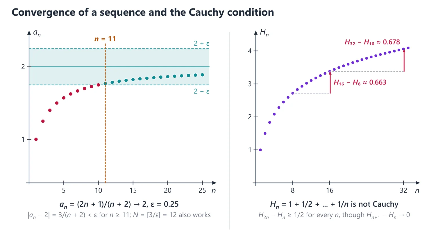
Non-example: an = log n has an+1 − an = log(1 + 1/n) → 0, yet a2n − an = log 2 for every n. With ε = log 2 and the pair m = 2n, the condition fails for every N, so (log n) is not Cauchy; indeed it tends to ∞.
Building up: (1) Convergent ⇒ Cauchy, by the ε/2 triangle inequality. (2) Cauchy ⇒ bounded (take ε = 1). (3) Bounded ⇒ a convergent subsequence (Bolzano–Weierstrass). (4) A Cauchy sequence with a convergent subsequence converges to the same limit (ε/2 again). Steps 1–4 are Standard Proofs, Theorem 4.
(5) A contractive sequence, |an+2 − an+1| ≤ k|an+1 − an| with k < 1, is Cauchy by a geometric-series bound (Theorem 17); this handles recursions an+1 = g(an) with decreasing g.
Where it is used: 'using Cauchy's general principle, examine the convergence of ...' is a direct UPSC question; the Cauchy criterion for series and for uniform convergence (and the M-test) are the same idea.
5. ℝ as a Complete Ordered Field
Ordered field: a field F with a relation < such that exactly one of a < b, a = b, b < a holds; a < b and b < c ⇒ a < c; a < b ⇒ a + c < b + c; and a < b, c > 0 ⇒ ac < bc.
Idea: ℚ and ℝ are ordered fields, but ℂ cannot be ordered. In any ordered field a square is never negative (if a < 0 then −a > 0 and a2 = (−a)2 > 0), so 1 = 12 > 0 and −1 < 0; then i2 = −1 would be a negative square.
Supremum: s = sup S if s is an upper bound of S and, for every ε > 0, there is x ∈ S with x > s − ε. The infimum is defined similarly.
Idea: sup S is the tightest ceiling over S: the ε-condition says the ceiling cannot be lowered by any amount without cutting into S. The supremum need not belong to S: sup (0, 1) = 1 ∉ (0, 1); when it does belong, it is the maximum.
Least upper bound (completeness) axiom: every non-empty subset of ℝ that is bounded above has a supremum in ℝ.
Idea: completeness says the real line has no holes. All the other field and order axioms already hold in ℚ, so this single axiom is what separates ℝ from ℚ, and every existence theorem of analysis (limits, maxima, integrals) ultimately rests on it.
ℚ is not complete: S = {x ∈ ℚ : x > 0, x2 < 2} is bounded above in ℚ but has no supremum in ℚ, since √2 is irrational.
Consequences: the Archimedean property (for x > 0 and any y there is n ∈ ℕ with nx > y); density of ℚ and of the irrationals in ℝ; the nested interval property.
Uniqueness: any two complete ordered fields are isomorphic, so ℝ is the complete ordered field.
6. Limit of a Sequence
Definition: an → l if for every ε > 0 there is N such that |an − l| < ε for all n ≥ N.
Idea: ε is the tolerance and N is the time after which the sequence stays within that tolerance; draw the band (l − ε, l + ε) and check that all but finitely many terms lie in it. Changing finitely many terms never affects convergence or the limit.
Finding N: for an = (2n + 1)/(n + 2), |an − 2| = 3/(n + 2) < ε as soon as n > 3/ε − 2, so N = [3/ε] works. Work backwards from |an − l| < ε, simplifying or bounding |an − l| from above.
Basic results: a limit is unique; every convergent sequence is bounded; limits respect sums, products and quotients (non-zero denominator); the sandwich theorem holds.
Monotone convergence theorem: a monotone sequence converges iff it is bounded; an increasing sequence bounded above converges to its supremum.
Idea: an increasing sequence bounded above has nowhere to go except up to its supremum (proved in Standard Proofs, Theorem 2). In ℚ this fails: 1, 1.4, 1.41, 1.414, ... increases and is bounded, but its limit √2 is not rational.
Bolzano–Weierstrass theorem: every bounded real sequence has a convergent subsequence.
Idea: bisect an interval containing the sequence; one half always contains infinitely many terms. The nested halves shrink to a point, and picking one term from each half gives a subsequence converging to it (Standard Proofs, Theorem 3). Boundedness is needed: an = n has no convergent subsequence.
Standard limits: n1/n → 1; a1/n → 1 (a > 0); (1 + 1/n)n → e; an → 0 for |a| < 1; nk/an → 0 for a > 1.
Cauchy's first theorem: if an → l then (a1 + a2 + ... + an)/n → l.
Idea: averaging cannot destroy convergence, but it can cure oscillation: (−1)n diverges while its averages tend to 0. So the converse of Cauchy's first theorem is false. The proof is in Standard Proofs, Theorem 5.
Cauchy's second theorem: if an > 0 and an → l then (a1a2...an)1/n → l. Consequently, if an > 0 and an+1/an → l then an1/n → l.
Upper and lower limits: a bounded sequence converges iff lim sup an = lim inf an, and then the limit is this common value.
Definition used in proofs: lim sup an = limn→∞ supk≥n ak, the limit of the decreasing sequence of tail suprema, and lim inf an = limn→∞ infk≥n ak. For an = (−1)n(1 + 1/n), lim sup = 1 and lim inf = −1, so the sequence diverges.
7. Cauchy Sequences and Completeness
Cauchy sequence: for every ε > 0 there is N with |am − an| < ε for all m, n ≥ N.
Idea: the terms become close to each other, and the definition never mentions a limit. That is its power: you can prove convergence when the limit is unknown. It is also where completeness enters, since the decimal approximations of √2 are Cauchy in ℚ but have no limit in ℚ.
Not the same as an+1 − an → 0: √n and Hn = 1 + 1/2 + ... + 1/n have consecutive differences tending to 0 but diverge; the Cauchy condition controls |am − an| for all m, n ≥ N, not only m = n + 1.
Results: every convergent sequence is Cauchy; every Cauchy sequence is bounded; a Cauchy sequence with a convergent subsequence converges.
Cauchy's general principle (completeness of ℝ): a real sequence converges iff it is a Cauchy sequence.
Contractive sequences: if |an+2 − an+1| ≤ k|an+1 − an| for all n with 0 < k < 1, then (an) is Cauchy and hence converges.
Why it works: |an+1 − an| ≤ kn−1|a2 − a1|, so for m > n, |am − an| ≤ (kn−1 + ... + km−2)|a2 − a1| ≤ kn−1|a2 − a1|/(1 − k) → 0 (Standard Proofs, Theorem 17). The same bound estimates the error |l − an|.
Equivalent forms of completeness: LUB property ⇔ monotone convergence theorem ⇔ Bolzano–Weierstrass ⇔ (Cauchy criterion together with the Archimedean property).
Example 1: Show that Hn = 1 + 1/2 + ... + 1/n is not a Cauchy sequence.
H2n − Hn = 1/(n + 1) + ... + 1/(2n) ≥ n·1/(2n) = 1/2 for every n, so the Cauchy condition fails for ε = 1/2, and Hn diverges.
Example 2: Let a1 = √2 and an+1 = √(2 + an). Show (an) converges and find its limit.
By induction an < 2: true for n = 1, and an < 2 ⇒ an+1 < √4 = 2. It is increasing, since an+12 − an2 = (2 − an)(1 + an) > 0. By the monotone convergence theorem an → l with l = √(2 + l), so l2 − l − 2 = 0 and l = 2 (l > 0).
Example 3: Find lim (n!)1/n/n.
Put an = n!/nn. Then an+1/an = (n/(n + 1))n = 1/(1 + 1/n)n → 1/e. By Cauchy's second theorem an1/n = (n!)1/n/n → 1/e.
8. Derivation: Density of ℚ and of the Irrationals
Let a < b. By the Archimedean property choose n ∈ ℕ with n(b − a) > 1. Let m = [na] + 1, so na < m ≤ na + 1 < nb. Dividing by n, a < m/n < b: there is a rational between any two reals.
Applying this to a/√2 < b/√2 gives a rational r ≠ 0 with a/√2 < r < b/√2 (if the first choice is r = 0, apply it again to (0, b/√2)), so a < r√2 < b and r√2 is irrational. Hence every interval contains both rationals and irrationals.
Use: density is what makes the Dirichlet function discontinuous everywhere and non-integrable (Continuity and Riemann Integral topics).
9. Derivation: (1 + 1/n)n Converges
By the binomial theorem, an = (1 + 1/n)n = ∑k=0n (1/k!)(1 − 1/n)(1 − 2/n)···(1 − (k − 1)/n).
Increasing: when n increases, each bracket (1 − j/n) increases and a new positive term is added, so an < an+1.
Bounded: every bracket is at most 1 and k! ≥ 2k−1, so an ≤ 1 + 1 + 1/2 + 1/4 + ... + 1/2n−1 < 3.
By the monotone convergence theorem the limit exists; it is called e, and 2 < e ≤ 3 (in fact e = 2.71828...).
10. Derivation: The Ratio Criterion for Sequences
Claim: if an > 0 and an+1/an → l < 1, then an → 0.
Proof: choose r with l < r < 1. For n ≥ N, an+1 ≤ ran, so an ≤ aNrn−N → 0. Similarly, if l > 1 then an → ∞.
Use: for an = nk/an (a > 1), an+1/an = (1 + 1/n)k/a → 1/a < 1, so nk/an → 0; for an = xn/n!, the ratio |x|/(n + 1) → 0, so xn/n! → 0 for every x.
11. Choosing the Method
If the limit is not known and only convergence is asked → Cauchy criterion, or monotone and bounded.
If two subsequences have different limits → the sequence diverges; this is the quickest proof of divergence for oscillating sequences.
If sup or inf of a set is asked → guess the value, prove it is a bound, then prove the ε-approximation (or find a sequence in the set tending to it); finally say whether it is attained.
12. Common Mistakes
Solving l = g(l) before proving convergence: for a1 = 1, an+1 = 2an, the equation l = 2l gives l = 0, yet an = 2n−1 → ∞. Prove convergence first, then find the limit.
Letting N depend on n: N may depend on ε (and on the sequence), never on the index n.
Confusing bounded with convergent, or Cauchy with an+1 − an → 0: (−1)n is bounded but divergent; √n has differences tending to 0 but is unbounded.
Assuming sup S ∈ S: say explicitly whether the supremum is attained (a maximum) or not.
Splitting limits that do not exist: lim anbn = lim an·lim bn needs both limits to exist; for an = 1/n, bn = n the product tends to 1 although lim bn does not exist.
Using Cauchy's second theorem without positivity: it needs an > 0; check this before taking n-th roots.
13. Connections
Link: completeness, through Bolzano–Weierstrass, gives the extreme value theorem and the Heine–Cantor theorem (Continuity topic), and hence the integrability of continuous functions (Riemann Integral topic).
Link: the contraction estimate is the convergence theory of fixed-point iteration xn+1 = g(xn) in Numerical Analysis: if g maps an interval into itself and |g′| ≤ k < 1 there, the iterates form a contractive sequence.
14. Worked Examples
Example 4: Find sup S and inf S for S = {1/m + 1/n : m, n ∈ ℕ}, and say whether they are attained.
Every element is at most 1 + 1 = 2, and 2 ∈ S (m = n = 1). So sup S = max S = 2.
Every element is positive, so 0 is a lower bound. Given ε > 0, choose n with n > 2/ε (Archimedean property); then 1/n + 1/n < ε, so ε is not a lower bound.
Hence inf S = 0, and it is not attained since 1/m + 1/n > 0.
Example 5: Prove that limn→∞ n1/n = 1.
For n ≥ 2 write n1/n = 1 + hn with hn ≥ 0.
By the binomial theorem n = (1 + hn)n ≥ (n(n − 1)/2)hn2, so hn2 ≤ 2/(n − 1).
Hence 0 ≤ hn ≤ √(2/(n − 1)) → 0, and by the sandwich theorem n1/n → 1.
Example 6: Let a1 = 1 and an+1 = 1/(1 + an). Show that (an) converges and find its limit.
By induction 1/2 ≤ an ≤ 1 for all n: true for n = 1, and if it holds for an then an+1 = 1/(1 + an) ∈ [1/2, 2/3].
|an+2 − an+1| = |an+1 − an|/((1 + an)(1 + an+1)) ≤ (4/9)|an+1 − an|, since each factor in the denominator is at least 3/2.
So (an) is contractive with k = 4/9, hence Cauchy, hence convergent (the sequence itself is not monotone: 1, 1/2, 2/3, 3/5, ...).
The limit l ≥ 1/2 satisfies l = 1/(1 + l), i.e. l2 + l − 1 = 0, so l = (√5 − 1)/2.
15. Topology of ℝ, Subsequences and Recursive Sequences
Neighbourhood, open and closed sets: a neighbourhood of c is a set containing some interval (c − δ, c + δ). G is open if it is a neighbourhood of each of its points, and F is closed if its complement is open.
Idea: an open set has elbow room around every point; a closed set contains every point it can be approached from. (0, 1) is open, [0, 1] is closed, and [0, 1) is neither, since 0 has no room and 1 is approached but missing.
Limit point: c is a limit point of S if every neighbourhood of c contains a point of S other than c. S is closed iff it contains all its limit points; the closure of S is S together with its limit points.
Bolzano–Weierstrass theorem for sets: every bounded infinite subset of ℝ has at least one limit point in ℝ. For example {1/n : n ∈ ℕ} has the single limit point 0, while the unbounded set ℕ has none.
Facts: arbitrary unions and finite intersections of open sets are open; ℚ is neither open nor closed; ∅ and ℝ are the only subsets of ℝ that are both open and closed.
Subsequences: if an → l, every subsequence converges to l. A number l is a limit point (cluster point) of (an) if some subsequence tends to l; for a bounded sequence lim sup an and lim inf an are the largest and smallest such points.
Sup and inf of a range: if f is monotone on an interval, the supremum and infimum of f are its values or one-sided limits at the end points; decide monotonicity from the sign of f′, and say whether each bound is attained.
Recursive sequences an+1 = g(an): (1) show the terms stay in an interval I with g(I) ⊆ I; (2) show monotonicity (if g is increasing on I, the sequence moves in the direction of a2 − a1); (3) apply the monotone convergence theorem and solve l = g(l). If g is decreasing, use the contraction estimate instead.
16. Solved Past UPSC Questions
Example 7 (UPSC 2016, 10 marks): Two sequences {xn} and {yn} are defined inductively by the following:
x1 = 1/2, y1 = 1 and xn = √(xn−1 yn−1), n = 2, 3, 4, ...
1/yn = (1/2)(1/xn + 1/yn−1), n = 2, 3, 4, ...
Prove that
xn−1 < xn < yn < yn−1, n = 2, 3, 4, ...
and deduce that both the sequences converge to the same limit l, where 1/2 < l < 1.
Claim: if 0 < xn−1 < yn−1, then xn−1 < xn < yn < yn−1. First, xn = √(xn−1yn−1) is the geometric mean of two unequal positive numbers, so xn−1 < xn < yn−1.
yn is the harmonic mean of xn and yn−1: yn = 2xnyn−1/(xn + yn−1). So yn − xn = xn(yn−1 − xn)/(xn + yn−1) > 0 and yn−1 − yn = yn−1(yn−1 − xn)/(xn + yn−1) > 0.
Since x1 = 1/2 < 1 = y1, induction gives xn−1 < xn < yn < yn−1 for all n ≥ 2.
So (xn) is increasing and bounded above by y1 = 1, and (yn) is decreasing and bounded below by x1 = 1/2. By the monotone convergence theorem xn → l and yn → m.
Letting n → ∞ in xn = √(xn−1yn−1) gives l = √(lm), so l2 = lm, and since l ≥ 1/2 > 0, l = m.
Finally x2 ≤ l ≤ y2, where x2 = 1/√2 > 1/2 and y2 < y1 = 1, so 1/2 < l < 1. (Numerically l = π/4 ≈ 0.785: this is Archimedes' polygon scheme for π.)
Answer: xn−1 < xn < yn < yn−1 for n ≥ 2, and both sequences converge to the same limit l with 1/2 < l < 1.
Example 8 (UPSC 2017, 10 marks): Find the supremum and the infimum of x/sin x on the interval (0, π/2].
Let f(x) = x/sin x on (0, π/2]. Then f′(x) = (sin x − x cos x)/sin2x, which equals cos x(tan x − x)/sin2x for x < π/2, and f′(π/2) = 1.
For 0 < x < π/2, tan x > x (g(x) = tan x − x has g(0) = 0 and g′(x) = sec2x − 1 > 0), so f′ > 0 and f is strictly increasing on (0, π/2].
Hence sup f = max f = f(π/2) = π/2.
inf f = limx→0+ x/sin x = 1, and it is not attained, because f is strictly increasing, so f(x) > 1 for every x in (0, π/2].
Answer: sup = π/2 (attained at x = π/2) and inf = 1 (not attained).
Example 9 (UPSC 2024, 15 marks): Using Cauchy's general principle of convergence, examine the convergence of the sequence ⟨fn⟩, where fn = 1 + 1/1! + 1/2! + … + 1/n!.
Cauchy's general principle: (fn) converges iff for every ε > 0 there is N with |fm − fn| < ε for all m > n ≥ N.
For m > n, |fm − fn| = 1/(n + 1)! + 1/(n + 2)! + ⋯ + 1/m!.
Since k! ≥ 2k−1 for k ≥ 1, this is at most 1/2n + 1/2n+1 + ⋯ + 1/2m−1 < 1/2n−1.
Given ε > 0 choose N with 1/2N−1 < ε; then |fm − fn| < ε for all m > n ≥ N, so (fn) is a Cauchy sequence.
By the completeness of ℝ (Cauchy's general principle) the sequence converges; its limit is e, with 2 < e < 3.
Answer: ⟨fn⟩ satisfies the Cauchy condition and therefore converges (to e).
17. Practice Exercises
Exercise 1 (basic): Find sup S and inf S for S = {(−1)n/n : n ∈ ℕ}, and say whether each is attained.
Answer: the elements are −1, 1/2, −1/3, 1/4, ...; sup S = 1/2 (attained at n = 2) and inf S = −1 (attained at n = 1).
Exercise 2 (basic): Using the ε–N definition, prove that (3n − 1)/(n + 4) → 3.
Answer: |an − 3| = 13/(n + 4) < ε when n > 13/ε − 4; N = [13/ε] + 1 works.
Exercise 3 (basic): Does an = (−1)n + 1/n converge? Find lim sup an and lim inf an.
Answer: the even terms tend to 1 and the odd terms to −1, so it diverges; lim sup = 1, lim inf = −1.
Exercise 4 (standard): Let a1 = 1 and an+1 = √(3 + 2an). Prove that (an) converges and find its limit.
Answer: by induction an < 3 and an+12 − an2 = (3 − an)(1 + an) > 0, so it is increasing and bounded; l2 = 3 + 2l gives l = 3.
Exercise 5 (standard): Find limn→∞ (nn/n!)1/n.
Answer: with bn = nn/n!, bn+1/bn = (1 + 1/n)n → e, so by Cauchy's second theorem the limit is e.
Exercise 6 (standard): Show directly from the definition that sn = ∑k=1n 1/k2 is a Cauchy sequence.
Answer: for m > n, sm − sn ≤ ∑k=n+1m (1/(k − 1) − 1/k) < 1/n; take N > 1/ε.
Exercise 7 (standard): Evaluate limn→∞ (1 + 21/2 + 31/3 + ... + n1/n)/n.
Answer: 1, by Cauchy's first theorem, since n1/n → 1.
Exercise 8 (UPSC level): Let a1 = 2 and an+1 = 2 + 1/an. Show that (an) is not monotone but converges, and find its limit.
Answer: terms 2, 2.5, 2.4, 2.4167, ... alternate; an ≥ 2 gives |an+2 − an+1| = |an+1 − an|/(anan+1) ≤ (1/4)|an+1 − an|, so it is contractive; l = 2 + 1/l gives l = 1 + √2.
Exercise 9 (UPSC level): Prove that bn = (1 + 1/n)n+1 is decreasing, and deduce its limit.
Answer: bn−1/bn = (1 + 1/(n2 − 1))n·n/(n + 1) ≥ (1 + n/(n2 − 1))·n/(n + 1) = (n3 + n2 − n)/(n3 + n2 − n − 1) > 1 by Bernoulli's inequality; bn = (1 + 1/n)n(1 + 1/n) → e.
Exercise 10 (UPSC level): Prove that xn = 1/(n + 1) + 1/(n + 2) + ... + 1/(2n) converges, and find its limit.
Answer: xn+1 − xn = 1/(2n + 1) − 1/(2n + 2) > 0 and xn < n·1/(n + 1) < 1, so it converges; as a Riemann sum of 1/(1 + x) on [0, 1] the limit is log 2.
| Form of the problem | Method | Watch out for |
|---|---|---|
| Rational function of n | Divide numerator and denominator by the highest power of n | Degrees: equal gives ratio of leading coefficients |
| an = f(n) with f differentiable | Find limx→∞ f(x) (L'Hospital), then restrict to n | The converse fails: sin(πn) → 0 but sin(πx) has no limit |
| (a1a2···an)1/n, (n!)1/n/n, an1/n | Cauchy's second theorem via an+1/an | Needs an > 0 |
| (a1 + ... + an)/n | Cauchy's first theorem | Converse false: (−1)n |
| (1/n)∑r=1n f(r/n) | Riemann sum: ∫01 f(x) dx | f must be integrable on [0, 1] |
| an+1 = g(an) | Bounded + monotone, or contraction; then l = g(l) | Prove convergence before solving l = g(l) |
| Sign changes, e.g. (−1)nbn | Even and odd subsequences | Different limits ⇒ divergence |
Mains points
- Standard questions: prove a recursively defined sequence converges (show bounded and monotone by induction, then solve the limit equation), or evaluate limits using Cauchy's first and second theorems.
- When asked to prove a sequence is or is not Cauchy, work directly with |am − an|; for divergence, exhibit a fixed ε and a pair m, n violating the condition.
- State the completeness axiom precisely and use ℚ (with √2) as the counter-example showing that an ordered field need not be complete.
- Common mistake: solving the limit equation before proving convergence; marks are given only after existence of the limit is established.
- Proofs of Bolzano–Weierstrass or the monotone convergence theorem from the LUB axiom are asked as short theory questions; keep the ε-argument tight.
Did you know?
- Dedekind (1872) built ℝ from 'cuts' of ℚ, and Cantor built it from Cauchy sequences of rationals in the same year; both constructions give the same complete ordered field.
Series: Convergence Tests, Absolute and Conditional Convergence, Rearrangement
A series converges when its partial sums converge, and an → 0 is necessary but not sufficient. Positive-term series are tested by comparison, ratio, root, Raabe, Gauss and condensation tests; alternating series by Leibniz's test. Absolutely convergent series (real or complex) can be rearranged freely, while a conditionally convergent real series can be rearranged to any sum (Riemann).
1. Understanding Partial Sums and the Meaning of ∑an
Why we need it: we cannot add infinitely many numbers one by one. Yet 1/2 + 1/4 + 1/8 + ... should equal 1, and 1 + 1 + 1 + ... should be 'infinite'. We need a definition that turns an endless sum into something we can test.
In words: the n-th partial sum Sn = a1 + ... + an is an ordinary finite sum. 'The series converges to S' means the sequence S1, S2, S3, ... converges to S. 'Diverges' means this sequence has no finite limit.
So there are always two sequences in play: the terms (an) and the partial sums (Sn). Do not confuse them: an → 0 is a statement about the terms; convergence is a statement about the partial sums.
First example, slowly: find the sum of ∑n=1∞ 1/(n(n + 1)).
Step 1 (partial fractions): 1/(n(n + 1)) = 1/n − 1/(n + 1).
Step 2 (write Sn): Sn = (1 − 1/2) + (1/2 − 1/3) + ... + (1/n − 1/(n + 1)).
Step 3 (cancel): every middle term cancels with its neighbour, leaving Sn = 1 − 1/(n + 1).
Step 4 (take the limit): Sn → 1, so the series converges and its sum is 1. Notice that we found the limit of the partial sums, not of the terms (the terms tend to 0).
Non-example: the harmonic series ∑1/n has terms tending to 0, but grouping S2k = 1 + 1/2 + (1/3 + 1/4) + (1/5 + ... + 1/8) + ... ≥ 1 + k/2 shows the partial sums are unbounded. The condition 'an → 0' is necessary but not sufficient.
Building up: (1) Since an = Sn − Sn−1, convergence forces an → 0. (2) Applying the Cauchy principle to (Sn) gives the Cauchy criterion: the blocks an+1 + ... + am must become small.
(3) If every an ≥ 0, (Sn) is increasing, so by the monotone convergence theorem the series converges iff the partial sums are bounded. Every test for positive series is a clever way of proving or disproving this bound.
Where it is used: telescoping sums appear in UPSC sums and in uniform convergence of series with closed-form Sn(x); the n-th term test is the fastest divergence proof.
2. Understanding Comparison with Known Series
Why we need it: most series cannot be summed in closed form, for example ∑(n + 1)/(n3 + 2). We decide convergence by comparing with a series whose behaviour we already know: the geometric series and the p-series ∑1/np.
In words: comparison test: if 0 ≤ an ≤ bn (from some n on) and the bigger series ∑bn converges, the smaller one converges; if the smaller one diverges, the bigger one diverges.
Limit form: if an, bn > 0 and an/bn → l with 0 < l < ∞, then eventually (l/2)bn < an < 2lbn, so the two series behave alike. The p-series rule: ∑1/np converges iff p > 1.
First example, slowly: test ∑(n + 1)/(n3 + 2).
Step 1 (positive terms): every term is positive, so comparison tests are allowed.
Step 2 (leading terms): for large n the numerator behaves like n and the denominator like n3, so an behaves like n/n3 = 1/n2. Choose bn = 1/n2.
Step 3 (the ratio): an/bn = (n3 + n2)/(n3 + 2) = (1 + 1/n)/(1 + 2/n3) → 1, which is finite and non-zero.
Step 4 (conclude): ∑1/n2 converges (p = 2 > 1), so by the limit comparison test the given series converges.
Non-example: comparing ∑1/(n + 1) with ∑1/n2 gives an/bn = n2/(n + 1) → ∞, which is outside 0 < l < ∞, so the limit form says nothing. The right comparison is bn = 1/n (ratio → 1), and the series diverges. The comparison series must have the correct power.
Building up: (1) Comparison follows from boundedness of partial sums: 0 ≤ a1 + ... + an ≤ b1 + ... + bn ≤ ∑bn. (2) The p-series rule follows from Cauchy's condensation test (Derivation 5 below), which compares ∑1/np with the geometric series ∑(21−p)k.
(3) For rational expressions in n, the power p is (degree of denominator) − (degree of numerator); for √ terms rationalise first, and for sin(1/n) or log(1 + 1/n) use sin t ~ t, log(1 + t) ~ t.
Where it is used: the first test to try for any positive series; it also settles the end points left open by the ratio test in power series.
3. Understanding the Ratio and Root Tests
Why we need it: terms like n!/nn or n5/3n are hard to compare with 1/np directly. If each term is roughly a fixed fraction of the previous one, the series behaves like a geometric series, and that is easy to decide.
In words: ratio test: compute l = lim an+1/an (terms positive). l < 1: converges; l > 1: diverges; l = 1: no information. Root test: the same with l = lim an1/n.
The number l is the 'effective common ratio' of the tail. When l = 1 the series is not like any geometric series, and the finer p-series tests (Raabe, Gauss, logarithmic) take over.
First example, slowly: test ∑n5/3n.
Step 1 (form the ratio): an+1/an = ((n + 1)5/3n+1)·(3n/n5) = (1/3)(1 + 1/n)5.
Step 2 (limit): (1 + 1/n)5 → 1, so l = 1/3.
Step 3 (meaning): pick r = 1/2, between 1/3 and 1. From some N on, each term is less than half of the previous one, so an ≤ aN(1/2)n−N.
Step 4 (conclude): the right side is a convergent geometric series, so ∑n5/3n converges by comparison. The polynomial factor n5 cannot beat the exponential 3n.
Non-example: for ∑1/n and ∑1/n2 the ratios n/(n + 1) and n2/(n + 1)2 both tend to 1, yet the first diverges and the second converges. So l = 1 is genuinely inconclusive; also 'every ratio is less than 1' is not enough, since n/(n + 1) < 1 always.
Building up: (1) Ratio test: l < r < 1 gives an ≤ Crn, and comparison finishes (Standard Proofs, Theorem 8). (2) Root test: an1/n < r gives an < rn directly.
(3) For l > 1 the terms eventually increase (or exceed 1), so an does not tend to 0. (4) When l = 1, Raabe's test compares with 1/np instead: n(an/an+1 − 1) → L, converge if L > 1, diverge if L < 1 (Derivation 6 below).
Where it is used: factorials and powers in UPSC series ∑(product)·xn: the ratio test fixes the range of x, Raabe or Gauss settles the boundary value; the same tests give the radius of convergence of power series.
4. Understanding Absolute and Conditional Convergence
Why we need it: when terms have both signs, positive-term tests do not apply directly, and cancellation can make a series converge although its sizes add up to ∞. We need to separate 'convergence by size' from 'convergence by cancellation'.
In words: ∑an is absolutely convergent if ∑|an| converges; then ∑an itself converges. It is conditionally convergent if ∑an converges but ∑|an| diverges.
Leibniz's test handles the commonest case: if un ≥ 0 decreases to 0, then u1 − u2 + u3 − ... converges, and the error after n terms is at most the first omitted term un+1.
First example, slowly: classify ∑(−1)n+1/(2n − 1) = 1 − 1/3 + 1/5 − ....
Step 1 (absolute values first): ∑1/(2n − 1) compared with ∑1/n gives ratio n/(2n − 1) → 1/2, finite and non-zero, so ∑|an| diverges. The series is not absolutely convergent.
Step 2 (Leibniz hypotheses): un = 1/(2n − 1) > 0; un+1 = 1/(2n + 1) < un, so it decreases; and un → 0.
Step 3 (conclude): by Leibniz the series converges, so it is conditionally convergent (its sum is π/4). Stopping after 100 terms gives an error below u101 = 1/201.
Non-example: ∑(−1)nn/(n + 1) alternates, but un = n/(n + 1) → 1, not 0. The Leibniz hypothesis un → 0 fails, and in fact the series diverges because its terms do not tend to 0.
Building up: (1) Absolute ⇒ ordinary convergence: |an+1 + ... + am| ≤ |an+1| + ... + |am|, then the Cauchy criterion (Standard Proofs, Theorem 6). (2) Leibniz: even partial sums increase, odd ones decrease, and they squeeze together (Theorem 7).
(3) Order matters only for conditional convergence: an absolutely convergent series has the same sum in every order, while a conditionally convergent real series can be rearranged to any sum, because its positive part and its negative part each diverge (Riemann, Theorem 18).
Where it is used: 'absolutely or conditionally convergent?' questions; error estimates for alternating series; rearrangement theory questions; power series at the end point x = −R.
5. Basic Facts
Convergence: ∑an converges to S if the partial sums Sn = a1 + ... + an converge to S.
Idea: a series is a sequence in disguise, the sequence of partial sums, so every theorem about sequences applies. For positive terms the partial sums increase, so ∑an converges iff its partial sums are bounded; every positive-term test is a way of proving that bound.
Necessary condition: if ∑an converges then an → 0; the harmonic series ∑1/n shows this is not sufficient.
Why it works: an = Sn − Sn−1 → S − S = 0. So 'an does not tend to 0' proves divergence at once, but 'an → 0' proves nothing.
Cauchy criterion: ∑an converges iff for every ε > 0 there is N with |an+1 + ... + am| < ε for all m > n ≥ N.
Standard series: the geometric series ∑rn converges iff |r| < 1; the p-series ∑1/np converges iff p > 1.
Why (geometric): for r ≠ 1, Sn = 1 + r + ... + rn−1 = (1 − rn)/(1 − r), which tends to 1/(1 − r) iff |r| < 1; for |r| ≥ 1 the terms do not tend to 0. The p-series is derived below by condensation.
6. Tests for Series of Positive Terms
Comparison test: if 0 ≤ an ≤ bn and ∑bn converges, then ∑an converges. Limit form: if an/bn → l with 0 < l < ∞, the two series converge or diverge together.
Idea: all positive-term tests are comparisons: the ratio and root tests compare with a geometric series, while Raabe, Gauss and the logarithmic test compare with p-series. That is why the ratio and root tests fail exactly when the series is 'slower than geometric', i.e. when the limit is 1.
D'Alembert's ratio test: if an+1/an → l, the series converges for l < 1 and diverges for l > 1; the test fails for l = 1.
Idea: if an+1/an → l < 1, the tail behaves like a geometric series of ratio about l (proved in Standard Proofs, Theorem 8). At l = 1 the test is silent: ∑1/n diverges and ∑1/n2 converges, yet both have ratio limit 1.
Cauchy's root test: if an1/n → l, the series converges for l < 1 and diverges for l > 1; it fails for l = 1.
Why it works: if an1/n → l < 1, choose r with l < r < 1; then an < rn for n ≥ N, and ∑rn converges. If l > 1, then an > 1 for large n, so an does not tend to 0.
Root is stronger than ratio: whenever an+1/an → l, also an1/n → l (Cauchy's second theorem), but not conversely. For an = 2−n+(−1)n the ratios alternate between 1/8 and 2, while an1/n → 1/2, so the root test proves convergence.
Raabe's test: if n(an/an+1 − 1) → l, the series converges for l > 1 and diverges for l < 1.
Gauss's test: if an/an+1 = 1 + μ/n + bn/np with p > 1 and (bn) bounded, the series converges iff μ > 1.
Logarithmic test: if n log(an/an+1) → l, the series converges for l > 1 and diverges for l < 1; it is convenient when an contains nn or (1 + 1/n)n.
Useful expansions: log(1 + 1/n)n = 1 − 1/(2n) + 1/(3n2) − ⋯, so e/(1 + 1/n)n = 1 + 1/(2n) + O(1/n2); Stirling's formula is n! ~ √(2πn) nne−n.
Series with a parameter x > 0: the ratio or root test gives convergence for x below some value and divergence above it; test the boundary value separately (Raabe, Gauss, logarithmic test or comparison).
Cauchy's condensation test: if (an) is positive and decreasing, ∑an and ∑2ka2k converge or diverge together; for example ∑1/(n(log n)p) converges iff p > 1.
Integral test: if f is positive and decreasing on [1, ∞), then ∑f(n) and ∫1∞ f(x) dx converge or diverge together.
Order of use: try an → 0, then comparison with a p-series, then ratio or root; if the ratio limit is 1, use Raabe, then Gauss or the logarithmic test.
7. Alternating Series, Absolute and Conditional Convergence
Leibniz test: if (un) is decreasing and un → 0, then ∑(−1)n+1un converges, and |S − Sn| ≤ un+1.
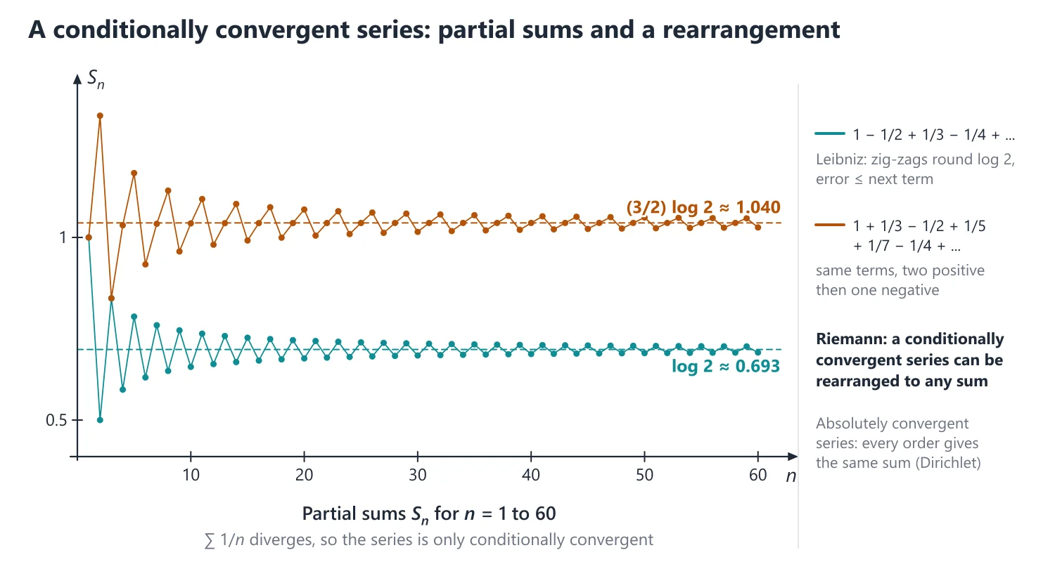
Idea: the partial sums zig-zag: S2 ≤ S4 ≤ S6 ≤ ... increase, S1 ≥ S3 ≥ S5 ≥ ... decrease, and the gap u2n+1 → 0 squeezes both to S, which lies between consecutive partial sums (hence the error bound). The proof is in Standard Proofs, Theorem 7.
Why monotonicity is needed: take u2k−1 = 1/k and u2k = 1/k2. Then un → 0, but the pairs give ∑(1/k − 1/k2), which diverges because ∑1/k diverges and ∑1/k2 converges.
Absolute convergence: if ∑|an| converges then ∑an converges. A series that converges but not absolutely is conditionally convergent, for example ∑(−1)n+1/n = log 2.
Idea: absolute convergence is convergence by size alone, so it survives any change of signs or order; conditional convergence depends on cancellation between positive and negative terms and is fragile. The implication is proved in Standard Proofs, Theorem 6.
Dirichlet's test: if the partial sums of ∑an are bounded and (bn) decreases monotonically to 0, then ∑anbn converges; so ∑sin(nx)/n converges for every real x.
Abel's test: if ∑an converges and (bn) is monotone and bounded, then ∑anbn converges.
Complex terms: ∑zn converges iff ∑Re zn and ∑Im zn both converge; if ∑|zn| converges then ∑zn converges; the ratio and root tests apply with |zn|.
8. Rearrangement of Series
Dirichlet's theorem: if ∑an converges absolutely, every rearrangement converges absolutely to the same sum.
Riemann's rearrangement theorem: if a real series ∑an converges conditionally, then for any real α (or ±∞) there is a rearrangement whose sum is α (or which diverges to ±∞).
Idea: in a conditionally convergent series the positive terms alone and the negative terms alone both have infinite sums. So you can climb above any target α using positive terms, fall below it using negative terms, and repeat; since an → 0 the overshoots shrink to 0 (Standard Proofs, Theorem 18).
Classic illustration: 1 − 1/2 + 1/3 − 1/4 + ... = log 2, while the rearrangement 1 + 1/3 − 1/2 + 1/5 + 1/7 − 1/4 + ... (two positive terms, one negative) has sum (3/2) log 2, and 1 − 1/2 − 1/4 + 1/3 − 1/6 − 1/8 + ... has sum (1/2) log 2.
Cauchy product (Mertens): if ∑an = A converges absolutely and ∑bn = B converges, then the Cauchy product ∑cn, cn = a0bn + a1bn−1 + ... + anb0, converges to AB.
Example 1: Test ∑an with an = (1·3·5...(2n − 1))/(2·4·6...(2n)) · 1/(2n + 1).
The ratio an+1/an → 1, so use Raabe. an/an+1 = (2n + 2)(2n + 3)/(2n + 1)2, so n(an/an+1 − 1) = n(6n + 5)/(2n + 1)2 → 6/4 = 3/2 > 1. The series converges.
Example 2: Discuss ∑(−1)n+1/√n.
un = 1/√n decreases to 0, so the series converges by Leibniz. But ∑1/√n is a p-series with p = 1/2 ≤ 1, which diverges. Hence the series is conditionally convergent.
Example 3: For which x > 0 does ∑xn/n converge?
an+1/an = nx/(n + 1) → x. It converges for x < 1 and diverges for x > 1; at x = 1 it is the harmonic series, which diverges.
9. Derivation: Cauchy's Condensation Test and the p-Series
Upper bound: let (an) be positive and decreasing. Grouping, a2 + a3 ≤ 2a2, a4 + ... + a7 ≤ 4a4, and so on, so S2k+1−1 ≤ ∑j=0k 2ja2j.
Lower bound: a3 + a4 ≥ 2a4, a5 + ... + a8 ≥ 4a8, and so on, so S2k ≥ (1/2)∑j=1k 2ja2j. The two bounds show that ∑an and ∑2ka2k are bounded together, hence converge together.
p-series: for an = 1/np (p > 0), 2ka2k = (21−p)k, a geometric series that converges iff 21−p < 1, i.e. p > 1. For p ≤ 0 the terms do not tend to 0.
10. Derivation: Raabe's Test from the p-Series
Ratio comparison lemma: if an, bn > 0 and an+1/an ≤ bn+1/bn for n ≥ N, then an/bn is decreasing from N on, so an ≤ Cbn; hence ∑bn convergent ⇒ ∑an convergent.
Convergence for l > 1: pick p with 1 < p < l and bn = 1/np. Then n(bn/bn+1 − 1) = n((1 + 1/n)p − 1) → p < l, so for large n, an/an+1 > bn/bn+1. Inverting gives the lemma's hypothesis, and ∑1/np converges.
Divergence for l < 1: for large n, n(an/an+1 − 1) < 1, i.e. an/an+1 < (n + 1)/n, so (n + 1)an+1 > nan. Thus nan ≥ c > 0 and an ≥ c/n, so ∑an diverges by comparison with the harmonic series.
11. Derivation: Abel's Summation and Dirichlet's Test
Summation by parts: with Ak = a1 + ... + ak, ∑k=n+1m akbk = Ambm − Anbn+1 + ∑k=n+1m−1 Ak(bk − bk+1), obtained by writing ak = Ak − Ak−1 and regrouping; it is the discrete form of integration by parts.
Dirichlet's test: if |Ak| ≤ M and bk decreases to 0, the right side is at most Mbm + Mbn+1 + M(bn+1 − bm) = 2Mbn+1 in absolute value, which tends to 0. By the Cauchy criterion ∑akbk converges.
Bounded trigonometric sums: for x ≠ 2kπ, |sin x + sin 2x + ... + sin nx| ≤ 1/|sin(x/2)|, from 2 sin(x/2) sin kx = cos((k − 1/2)x) − cos((k + 1/2)x), which telescopes. This is the bound used for ∑sin(nx)/n and ∑cos(nx)/n.
12. Choosing the Method
If the terms have both signs → test ∑|an| first; if that diverges, use Leibniz (alternating) or Dirichlet/Abel, and then state 'conditionally convergent'.
If the series contains a parameter x → ratio or root test for the range of x, then test the boundary values separately by another test.
13. Common Mistakes
Concluding convergence from an → 0: the harmonic series is the standard counter-example.
Reading the ratio test as 'an+1/an < 1 ⇒ convergence': for ∑1/n the ratio n/(n + 1) is always less than 1. The ratio must stay below some fixed r < 1, which is what l < 1 guarantees.
Applying positive-term tests to series with negative terms: comparison, Raabe and Gauss need an ≥ 0; for mixed signs apply them to |an|.
Skipping the 'decreasing' check in Leibniz: show un+1 ≤ un (for example by the sign of the derivative of u(x)), not only un → 0.
Regrouping or reordering freely: brackets may be inserted into a convergent series, but removing brackets or reordering can change the answer: (1 − 1) + (1 − 1) + ... = 0, while 1 − 1 + 1 − 1 + ... diverges.
14. Connections
Link: the radius of convergence of a power series comes from the root and ratio tests (Uniform Convergence topic), and the same tests decide the regions of convergence of Taylor and Laurent series in Complex Analysis.
Link: the integral test ties series to improper integrals (Riemann Integral topic): ∑1/np and ∫1∞ dx/xp converge for the same p, and Dirichlet's test has an exact integral analogue.
15. Worked Examples
Example 4: Test the convergence of ∑(1 + 1/n)−n2.
Use the root test: an1/n = (1 + 1/n)−n = 1/(1 + 1/n)n.
Since (1 + 1/n)n → e, an1/n → 1/e < 1.
Hence the series converges by Cauchy's root test.
Example 5: Test ∑n≥2 1/(n log n) and ∑n≥2 1/(n(log n)2).
Both terms are positive and decreasing, so the integral test applies on [2, ∞).
∫2X dx/(x log x) = log(log X) − log(log 2) → ∞, so ∑1/(n log n) diverges.
∫2X dx/(x(log x)2) = 1/log 2 − 1/log X → 1/log 2, so ∑1/(n(log n)2) converges. (Cauchy's condensation test gives the same: it reduces them to ∑1/(k log 2) and ∑1/(k2(log 2)2).)
Example 6: Show that ∑cos(nx)/n converges for every x that is not a multiple of 2π, and diverges when x = 2kπ.
For x ≠ 2kπ, sin(x/2) ≠ 0 and 2 sin(x/2)∑k=1n cos kx = sin((n + 1/2)x) − sin(x/2), so |∑k=1n cos kx| ≤ 1/|sin(x/2)| for every n.
The partial sums of ∑cos(nx) are therefore bounded, and 1/n decreases monotonically to 0.
By Dirichlet's test, ∑cos(nx)/n converges. When x = 2kπ every cos(nx) = 1 and the series is the divergent harmonic series.
Example 7: Test ∑an with an = ((1·3·5...(2n − 1))/(2·4·6...(2n)))2.
an/an+1 = ((2n + 2)/(2n + 1))2 → 1, so the ratio test fails; Raabe gives n(an/an+1 − 1) = n(4n + 3)/(2n + 1)2 → 1, so Raabe also fails.
Use Gauss: an/an+1 = (1 + 1/(2n + 1))2 = 1 + 1/n + bn/n2, where bn = n2[1/(2n + 1)2 − 1/(n(2n + 1))] is bounded (it tends to −1/4).
Here μ = 1, which is not greater than 1, so the series diverges by Gauss's test.
Example 8: Show that the complex series ∑n=1∞ in/n converges, but not absolutely.
Even n = 2k give the real part ∑(−1)k/(2k) = −1/2 + 1/4 − 1/6 + ⋯, convergent by Leibniz (to −(1/2) log 2).
Odd n = 2k − 1 give the imaginary part ∑(−1)k−1/(2k − 1) = 1 − 1/3 + 1/5 − ⋯, convergent by Leibniz (to π/4).
Both parts converge, so ∑in/n converges (to −(1/2) log 2 + iπ/4); but ∑|in/n| = ∑1/n diverges, so the convergence is conditional.
16. Solved Past UPSC Questions
Example 9 (UPSC 2022, 15 marks): Test for convergence or divergence of the series x + 22x2/2! + 33x3/3! + 44x4/4! + 55x5/5! + ⋯ (x > 0)
an = nnxn/n! > 0, and an+1/an = (n + 1)n+1x/((n + 1)nn) = (1 + 1/n)nx → ex.
By the ratio test the series converges for ex < 1, i.e. 0 < x < 1/e, and diverges for x > 1/e.
At x = 1/e the ratio tends to 1. Using log(1 + 1/n)n = 1 − 1/(2n) + 1/(3n2) − ⋯, an/an+1 = e/(1 + 1/n)n = 1 + 1/(2n) + O(1/n2).
So n(an/an+1 − 1) → 1/2 < 1, and the series diverges by Raabe's test (Stirling's formula agrees: an ~ 1/√(2πn)).
Answer: convergent for 0 < x < 1/e and divergent for x ≥ 1/e.
Example 10 (UPSC 2023, 10 marks): Test the convergence of the series ∑n=1∞ [1.3.5 … (2n − 1)]/[2.4.6 … (2n)] · x2n+1/(2n + 1), x > 0
Let an = (1·3···(2n − 1))/(2·4···(2n)) · x2n+1/(2n + 1). Then an+1/an = ((2n + 1)/(2n + 2))·((2n + 1)/(2n + 3))·x2 → x2.
By the ratio test the series converges for 0 < x < 1 and diverges for x > 1.
At x = 1, an/an+1 = (2n + 2)(2n + 3)/(2n + 1)2, so n(an/an+1 − 1) = n(6n + 5)/(2n + 1)2 → 3/2 > 1, and the series converges by Raabe's test.
Answer: convergent for 0 < x ≤ 1 and divergent for x > 1 (for 0 < x ≤ 1 the sum is sin−1x − x).
17. Practice Exercises
Exercise 1 (basic): Does ∑n/(2n + 1) converge?
Answer: no; its terms tend to 1/2 ≠ 0, so it diverges by the n-th term test.
Exercise 2 (basic): Find the sum of ∑n=1∞ 1/(n2 + 3n + 2).
Answer: 1/((n + 1)(n + 2)) = 1/(n + 1) − 1/(n + 2) telescopes, giving Sn = 1/2 − 1/(n + 2) → 1/2.
Exercise 3 (basic): Find the sum of ∑n=0∞ (2/3)n.
Answer: a geometric series with ratio 2/3 < 1; the sum is 1/(1 − 2/3) = 3.
Exercise 4 (standard): Test ∑(√(n + 1) − √n)/n.
Answer: the term is 1/(n(√(n + 1) + √n)), which behaves like 1/(2n3/2); converges by limit comparison with ∑1/n3/2.
Exercise 5 (standard): Test ∑n!/nn.
Answer: an+1/an = (n/(n + 1))n → 1/e < 1; converges by the ratio test.
Exercise 6 (standard): Test ∑(n/(n + 1))n2.
Answer: an1/n = 1/(1 + 1/n)n → 1/e < 1; converges by the root test.
Exercise 7 (standard): For which x > 0 does ∑xn/n2 converge?
Answer: the ratio tends to x: convergent for x < 1, divergent for x > 1, and at x = 1 it is ∑1/n2, convergent; so exactly for 0 < x ≤ 1.
Exercise 8 (UPSC level): Is ∑(−1)n+1n/(n2 + 1) absolutely convergent, conditionally convergent or divergent?
Answer: conditionally convergent: u(x) = x/(x2 + 1) has u′(x) = (1 − x2)/(x2 + 1)2 ≤ 0 for x ≥ 1 and un → 0 (Leibniz), while un/(1/n) → 1 makes ∑un diverge.
Exercise 9 (UPSC level): Test ∑n≥1 (1·2·3···n)/(3·5·7···(2n + 1)) xn, x > 0.
Answer: an+1/an = (n + 1)x/(2n + 3) → x/2; at x = 2, n(an/an+1 − 1) = n/(2n + 2) → 1/2 < 1 (Raabe). Convergent for 0 < x < 2, divergent for x ≥ 2.
Exercise 10 (UPSC level): Test ∑1/n1+1/n, and explain why the ratio and root tests cannot decide it.
Answer: both limits equal 1; but an/(1/n) = 1/n1/n → 1, so it diverges by limit comparison with the harmonic series.
| Test | Compute | Converges if | Diverges if |
|---|---|---|---|
| Ratio (D'Alembert) | l = lim an+1/an | l < 1 | l > 1 |
| Root (Cauchy) | l = lim an1/n | l < 1 | l > 1 |
| Raabe | l = lim n(an/an+1 − 1) | l > 1 | l < 1 |
| Logarithmic | l = lim n log(an/an+1) | l > 1 | l < 1 |
| Gauss | an/an+1 = 1 + μ/n + O(1/np), p > 1 | μ > 1 | μ ≤ 1 |
| p-series ∑1/np | p | p > 1 | p ≤ 1 |
| Form of the series | Test | Watch out for |
|---|---|---|
| an does not tend to 0 | n-th term test: diverges | Only a test for divergence |
| Algebraic in n, e.g. (n + 1)/(n3 + 2) | Limit comparison with 1/np, p = (degree of denominator) − (degree of numerator) | Use the leading terms only |
| Factorials, an, nk | Ratio test | Limit 1 decides nothing |
| an = (bn)n | Root test | Use (1 + c/n)n → ec |
| Ratio → 1, products like 1·3·5···/(2·4·6···) | Raabe, then Gauss | Raabe limit 1 also fails; go to Gauss |
| Terms with nn, (1 + 1/n)n, en | Logarithmic test | Expand log(1 + 1/n) to two terms |
| 1/(n(log n)p), decreasing f(n) | Condensation or integral test | Needs positive decreasing terms |
| (−1)nun | Leibniz; then check ∑un | Prove un decreasing |
| sin(nx)/np, cos(nx)/np | p > 1: comparison with 1/np; 0 < p ≤ 1: Dirichlet | x = 2kπ needs separate treatment for cosines |
Mains points
- Typical questions: test the convergence of a given series, often of the form ∑(product of factors)·xn, where the ratio test settles x ≠ 1 and Raabe or Gauss settles x = 1.
- Always name the test you use and state its hypotheses (positive terms, monotone decrease, limit value); a bare computation without naming the test loses marks.
- For 'absolutely or conditionally convergent' questions, test ∑|an| first; if it diverges, apply Leibniz or Dirichlet to the original series.
- Rearrangement questions ask you to state Riemann's theorem and illustrate it with the alternating harmonic series; mention that absolute convergence makes the sum independent of order.
- Common mistake: using an → 0 to claim convergence, or applying the ratio test when its limit is 1.
Did you know?
- The harmonic series diverges extremely slowly: its partial sums need more than 12000 terms to pass 10, since Hn ≈ log n + 0.5772 (Euler's constant).
Continuity, Uniform Continuity and Continuous Functions on Compact Sets
A function is continuous at c if f(x) → f(c) as x → c, and uniformly continuous if one δ works for every point of the domain. On a compact set (closed and bounded in ℝn) a continuous function is bounded, attains its maximum and minimum, and is uniformly continuous; on an interval it also has the intermediate value property.
1. Understanding ε–δ Continuity
Why we need it: 'a graph drawn without lifting the pen' is a picture, not a proof. For functions like x sin(1/x) or functions defined differently on ℚ and on the irrationals, the picture fails, and we need a definition we can check line by line.
In words: f is continuous at c if: for every ε > 0 (how close you want f(x) to be to f(c)) there is δ > 0 (how close x must be to c) such that every x in the domain with |x − c| < δ satisfies |f(x) − f(c)| < ε.
Equivalently, limx→c f(x) exists and equals f(c). Three things must happen: f(c) is defined, the limit exists, and the two are equal.
First example, slowly: prove that f(x) = 3x + 1 is continuous at c = 2.
Step 1 (write the gap): |f(x) − f(2)| = |3x + 1 − 7| = 3|x − 2|.
Step 2 (what we need): 3|x − 2| < ε, i.e. |x − 2| < ε/3.
Step 3 (choose δ): δ = ε/3. For ε = 0.03 this is δ = 0.01: every x in (1.99, 2.01) has f(x) in (6.97, 7.03).
Step 4 (check): |x − 2| < δ ⇒ |f(x) − 7| = 3|x − 2| < 3δ = ε. Done.
For a non-linear f, first restrict x (say |x − c| < 1) to bound the extra factor, and take δ as the minimum of 1 and the δ that the bound gives, as in δ = min(1, ε/(2|c| + 1)) for x2.
Non-example: f(x) = 1 for x ≥ 0 and f(x) = 0 for x < 0 is not continuous at 0. Take ε = 1/2: every interval (−δ, δ) contains a negative x with |f(x) − f(0)| = 1 > 1/2, so no δ works.
Building up: (1) Sums, products, quotients (non-zero denominator) and compositions of continuous functions are continuous, by the same inequalities as for sequences. (2) The sequential criterion: f is continuous at c iff xn → c ⇒ f(xn) → f(c).
(3) The criterion turns every sequence theorem into a continuity theorem, and gives the easiest disproof: two sequences tending to c with different limits of f(xn). (4) Rational/irrational definitions are handled by a rational and an irrational sequence tending to c.
Where it is used: continuity of piecewise functions at junctions, classification of discontinuities, and every theorem on [a, b] below; the same ε–δ pattern gives limits in two variables.
2. Understanding Continuous Functions on [a, b]
Why we need it: to know that an equation has a root, or that an optimisation problem has an answer, we need guarantees: a maximum exists, every intermediate value is taken. Continuity alone does not give them; the closed bounded interval does.
In words: on [a, b], a continuous f is bounded (|f(x)| ≤ M for some M), attains its maximum and minimum (there are points where f equals sup f and inf f), and takes every value between f(a) and f(b) (intermediate value theorem).
'Closed' means the end points are included; 'bounded' means the interval is finite. More generally these hold on any compact set (closed and bounded in ℝn), except the intermediate value property, which needs an interval.
First example, slowly: show that x5 − 3x − 1 = 0 has a root between 1 and 2, and find it to one decimal place.
Step 1 (continuity): f(x) = x5 − 3x − 1 is a polynomial, hence continuous on [1, 2].
Step 2 (signs at the ends): f(1) = 1 − 3 − 1 = −3 < 0 and f(2) = 32 − 6 − 1 = 25 > 0.
Step 3 (IVT): 0 lies between −3 and 25, so f(c) = 0 for some c ∈ (1, 2).
Step 4 (bisect): f(1.5) ≈ 2.09 > 0, so c ∈ (1, 1.5); f(1.3) ≈ −1.19 < 0 and f(1.4) ≈ 0.18 > 0, so c ∈ (1.3, 1.4); f(1.35) ≈ −0.57 < 0 puts c ∈ (1.35, 1.4), so c ≈ 1.4 to one decimal place (in fact c ≈ 1.389).
Non-example: f(x) = x on the open interval (0, 1) is continuous and bounded but never reaches its supremum 1: the end point 1 is missing, so 'closed' fails. f(x) = x on [0, ∞) is unbounded: 'bounded interval' fails.
Building up: (1) Boundedness: if not, pick xn with |f(xn)| > n; Bolzano–Weierstrass gives xnk → c ∈ [a, b] (closedness keeps c inside), and continuity makes f(xnk) bounded, a contradiction (Standard Proofs, Theorem 9).
(2) Attaining the maximum: choose f(yn) > M − 1/n and repeat the subsequence argument. (3) IVT: c = sup{x : f(x) < k} cannot have f(c) < k or f(c) > k (Theorem 10).
Where it is used: existence and uniqueness of roots (IVT plus monotonicity), fixed-point questions, absolute extrema; in Numerical Analysis the bisection method is the IVT made into an algorithm.
3. Understanding Uniform Continuity
Why we need it: in ordinary continuity δ may change from point to point. To control f on a whole interval at once (for example to show that a continuous function is integrable), we need one δ that works everywhere.
In words: f is uniformly continuous on E if for every ε > 0 there is a δ > 0, chosen before any point is named, such that any two points x, y of E closer than δ have f-values closer than ε.
Compare the quantifiers: continuity is 'for every c, for every ε, there is δ(ε, c)'; uniform continuity is 'for every ε, there is δ(ε), for every x, y'. Moving 'there is δ' before 'for every point' is the whole difference.
First example, slowly: show f(x) = 1/x is uniformly continuous on [1, ∞).
Step 1 (difference): |1/x − 1/y| = |x − y|/(xy).
Step 2 (bound the extra factor uniformly): x, y ≥ 1 gives xy ≥ 1, so |1/x − 1/y| ≤ |x − y|. The bound does not depend on where x and y are.
Step 3 (choose δ): δ = ε. Then |x − y| < δ ⇒ |f(x) − f(y)| < ε for all x, y ≥ 1.
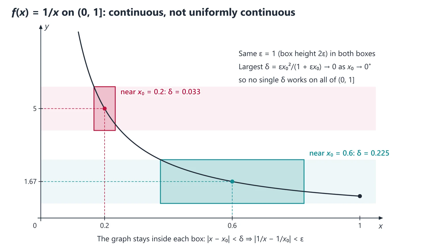
Step 4 (notice): on (0, 1] the same computation gives |x − y|/(xy) with xy as small as we like, so no single δ can work there; the domain matters as much as the formula.
Non-example: f(x) = x2 on ℝ is continuous at every point but not uniformly continuous. With xn = n + 1/n and yn = n the inputs get closer (|xn − yn| = 1/n) while the outputs stay more than 2 apart, so the condition fails for ε = 2.
Building up: (1) Lipschitz ⇒ uniformly continuous with δ = ε/L; a bounded derivative on an interval gives a Lipschitz bound by the mean value theorem. (2) Heine–Cantor: continuous on [a, b] ⇒ uniformly continuous, by contradiction with Bolzano–Weierstrass (Standard Proofs, Theorem 11).
(3) Negation: not uniformly continuous iff there are ε0 and pairs xn, yn with |xn − yn| → 0 and |f(xn) − f(yn)| ≥ ε0. (4) On a bounded open interval, uniformly continuous iff f extends continuously to the end points.
Where it is used: 'prove or disprove uniform continuity' questions; integrability of continuous functions (Riemann Integral topic); uniform convergence arguments use the same 'one N for all x' idea.
4. Continuity
ε-δ definition: f is continuous at c if for every ε > 0 there is δ > 0 such that |x − c| < δ ⇒ |f(x) − f(c)| < ε.
Idea: whatever output tolerance ε is demanded, some input tolerance δ meets it: over (c − δ, c + δ) the graph stays inside a box of height 2ε centred at (c, f(c)). Here δ may depend on both ε and the point c.
Finding δ: for f(x) = x2 at c, if |x − c| < 1 then |x + c| ≤ 2|c| + 1, so |x2 − c2| = |x − c||x + c| ≤ (2|c| + 1)|x − c|. Hence δ = min(1, ε/(2|c| + 1)) works. This δ shrinks as |c| grows, which is the first sign that x2 is not uniformly continuous on ℝ.
Sequential criterion: f is continuous at c iff xn → c implies f(xn) → f(c) for every sequence (xn) in the domain.
Use: it is the quickest way to disprove continuity. For sin(1/x) at 0 (with any value at 0), xn = 1/(nπ) gives f(xn) = 0 and yn = 1/(2nπ + π/2) gives f(yn) = 1; two sequences tending to 0 with different limits of f show that limx→0 f(x) does not exist.
Types of discontinuity: removable (limit exists but ≠ f(c) or f(c) undefined); first kind or jump (both one-sided limits exist but differ); second kind (at least one one-sided limit fails to exist).
Monotone functions: a monotone function on an interval has only jump discontinuities, and at most countably many of them.
Why countably many: at each jump c the open interval (f(c−), f(c+)) is non-empty, intervals at different jumps are disjoint (by monotonicity), and each contains a rational. Choosing one rational per jump gives a one-one map from the jumps into ℚ.
Standard examples: the Dirichlet function (1 on ℚ, 0 elsewhere) is discontinuous everywhere; x sin(1/x) with value 0 at 0 is continuous at 0; Thomae's function (1/q at p/q in lowest terms, 0 at irrationals) is continuous exactly at the irrationals.
5. Continuous Functions on Compact Sets
Compactness: K is compact if every open cover of K has a finite subcover. Heine–Borel theorem: a subset of ℝn is compact iff it is closed and bounded; equivalently, every sequence in K has a subsequence converging in K.
Idea: compact means 'finite in disguise': local information (near each point f is bounded) becomes global because finitely many neighbourhoods suffice. On (0, 1], which is not closed, the continuous function 1/x is bounded near each point but not on the whole set.
Boundedness theorem: a continuous function on a compact set is bounded.
Extreme value theorem: a continuous real function on a non-empty compact set attains its supremum and infimum.
Why each hypothesis is needed: on (0, 1), f(x) = x has supremum 1 but never reaches it (not closed); on ℝ, f(x) = x is unbounded (not bounded); on [−1, 1], f(x) = 1/x for x ≠ 0 with f(0) = 0 is unbounded (not continuous). The proof is in Standard Proofs, Theorem 9.
Image theorem: the continuous image of a compact set is compact, and the continuous image of a connected set (an interval in ℝ) is connected.
Intermediate value theorem: if f is continuous on [a, b] and k lies between f(a) and f(b), then f(c) = k for some c ∈ [a, b].
Idea: a continuous graph cannot jump over a horizontal line. Both continuity and the interval matter: the sign function jumps over 0 on [−1, 1], and on the disconnected set [0, 1] ∪ [2, 3] the function equal to 0 then 1 is continuous but skips 1/2. The proof by bisection is in Standard Proofs, Theorem 10.
Inverse function: a continuous bijection from a compact set onto its image has a continuous inverse; a continuous one-one function on an interval is strictly monotone.
Fixed point: every continuous f : [a, b] → [a, b] has a fixed point (apply the IVT to f(x) − x).
Why it works: g(x) = f(x) − x is continuous with g(a) = f(a) − a ≥ 0 and g(b) = f(b) − b ≤ 0, because f takes values in [a, b]; the IVT gives c with g(c) = 0.
6. Uniform Continuity
Definition: f is uniformly continuous on E if for every ε > 0 there is δ > 0, depending only on ε, such that x, y ∈ E and |x − y| < δ ⇒ |f(x) − f(y)| < ε.
Idea: one δ must serve the whole domain at once. See the figure above: for 1/x on (0, 1) the graph gets steeper near 0, so an input window of fixed width δ produces larger and larger output jumps as it slides to the left, and no single δ works. On [a, ∞) with a > 0 the slope is at most 1/a2, and δ = a2ε works everywhere.
Heine–Cantor theorem: a function continuous on a compact set is uniformly continuous there.
Sufficient conditions: a Lipschitz function (|f(x) − f(y)| ≤ L|x − y|) is uniformly continuous; a differentiable function with bounded derivative on an interval is Lipschitz, by the mean value theorem.
Why it works: by the mean value theorem |f(x) − f(y)| = |f′(ξ)||x − y| ≤ M|x − y|, so δ = ε/M works. The converse fails: √x is uniformly continuous on [0, ∞), since |√x − √y| ≤ √|x − y| gives δ = ε2, although its derivative is unbounded near 0.
Test for failure: f is not uniformly continuous on E iff there exist ε0 > 0 and sequences xn, yn in E with |xn − yn| → 0 but |f(xn) − f(yn)| ≥ ε0.
Why it works: this is the logical negation of the definition: 'there is an ε0 such that every δ fails' becomes, with δ = 1/n, a pair xn, yn with |xn − yn| < 1/n and |f(xn) − f(yn)| ≥ ε0. For x2 on ℝ take xn = n + 1/n, yn = n: the difference of squares is 2 + 1/n2 > 2.
Properties: a uniformly continuous function maps Cauchy sequences to Cauchy sequences; f is uniformly continuous on a bounded open interval (a, b) iff it extends to a continuous function on [a, b].
Unbounded domains: if f is continuous on [a, ∞) and limx→∞ f(x) exists finitely, then f is uniformly continuous on [a, ∞); likewise on ℝ when both limits at ±∞ exist. A continuous periodic function is uniformly continuous on ℝ.
Continuous extension: a function continuous on (a, b) with finite one-sided limits at a and b extends continuously to [a, b]. For example x2 sin(1/x) extends by the value 0 at x = 0, and the extension is even differentiable there.
Standard cases: √x on [0, ∞) and sin x on ℝ are uniformly continuous; x2 on ℝ, 1/x on (0, 1) and sin(1/x) on (0, 1) are not; 1/x on [a, ∞) with a > 0 is.
7. Derivation: Extension Theorem and Unbounded Domains
Uniformly continuous on (a, b) ⇒ extends to [a, b]: let xn → a in (a, b). Then (xn) is Cauchy, so (f(xn)) is Cauchy (uniform continuity) and converges. If xn → a and yn → a, the interleaved sequence x1, y1, x2, y2, ... also tends to a, so both limits agree. Defining f(a) as this limit (and f(b) similarly) gives a continuous extension.
Consequence: sin(1/x) and 1/x are not uniformly continuous on (0, 1), because they have no finite limit at 0; x sin(1/x) is, because it tends to 0.
Continuous on [a, ∞) with a finite limit L at ∞ ⇒ uniformly continuous: given ε, choose M with |f(x) − L| < ε/2 for x ≥ M, so |f(x) − f(y)| < ε for x, y ≥ M. On the compact [a, M + 1] Heine–Cantor gives δ1. With δ = min(δ1, 1), two points with |x − y| < δ either both lie in [a, M + 1] or both lie in [M, ∞), and in each case |f(x) − f(y)| < ε.
8. Derivation: Continuous Image of a Compact Set
Let yn = f(xn) be any sequence in f(K). Since K is compact, a subsequence xnk → x ∈ K, and by continuity ynk = f(xnk) → f(x) ∈ f(K). So every sequence in f(K) has a subsequence converging in f(K): f(K) is compact.
A compact subset of ℝ is closed and bounded, so it has a largest and a smallest element; this re-proves the extreme value theorem.
9. Choosing the Method
If continuity of a piecewise function at a junction is asked → compute both one-sided limits and compare with f(c); for oscillating factors such as x sin(1/x) use the sandwich bound |x sin(1/x)| ≤ |x|.
If you must disprove continuity → two sequences tending to c along which f has different limits (or a limit different from f(c)).
If you must prove uniform continuity → compact domain: Heine–Cantor; bounded derivative: Lipschitz; [a, ∞) with a finite limit at ∞: the derivation above; otherwise a direct estimate such as |√x − √y| ≤ √|x − y|.
If you must disprove uniform continuity → a pair of sequences with |xn − yn| → 0 but |f(xn) − f(yn)| ≥ ε0; or a Cauchy sequence mapped to a non-Cauchy one; or, on a bounded interval, f unbounded or without a finite end-point limit.
If a root must be shown to exist → IVT on a sign change; for uniqueness add strict monotonicity (f′ > 0 or f′ < 0).
10. Common Mistakes
Letting δ depend on the point when proving uniform continuity: δ = ε/(2|c| + 1) proves continuity of x2, not uniform continuity.
Assuming continuity on an open or unbounded set gives uniform continuity: 1/x on (0, 1) and x2 on ℝ are the standard counter-examples.
Thinking 'unbounded derivative ⇒ not uniformly continuous': √x on [0, 1] is uniformly continuous (Heine–Cantor) although f′(x) → ∞ as x → 0.
Thinking 'bounded ⇒ uniformly continuous': sin(1/x) on (0, 1) is bounded and continuous but not uniformly continuous.
Applying the IVT where f is not continuous on the whole closed interval: tan(π/4) = 1 > 0 and tan(3π/4) = −1 < 0, yet tan x has no zero in [π/4, 3π/4], because it is discontinuous at π/2.
11. Connections
Link: Heine–Cantor is the key step in proving that continuous functions are Riemann integrable (Riemann Integral topic): on short sub-intervals the oscillation is uniformly small.
Link: the IVT is the basis of the bisection method in Numerical Analysis, and the extreme value theorem on closed bounded regions justifies the search for absolute extrema in the Several Variables topic.
12. Worked Examples
Example 1: Show that f(x) = x2 is uniformly continuous on [0, 1] but not on ℝ.
On [0, 1], |x2 − y2| = |x + y||x − y| ≤ 2|x − y|, so δ = ε/2 works. On ℝ take xn = n + 1/n and yn = n: |xn − yn| = 1/n → 0 but xn2 − yn2 = 2 + 1/n2 ≥ 2, so f is not uniformly continuous.
Example 2: Show that f(x) = 1/(1 + x2) is uniformly continuous on ℝ.
f′(x) = −2x/(1 + x2)2, and 2|x| ≤ 1 + x2 ≤ (1 + x2)2, so |f′(x)| ≤ 1. By the mean value theorem |f(x) − f(y)| ≤ |x − y|, and δ = ε works.
Example 3: Show that x3 + x − 1 = 0 has exactly one real root, and it lies in (0, 1).
f(x) = x3 + x − 1 is continuous with f(0) = −1 < 0 and f(1) = 1 > 0, so by the IVT a root lies in (0, 1). Since f′(x) = 3x2 + 1 > 0, f is strictly increasing, so the root is unique.
Example 4: Show that f(x) = sin(1/x) is not uniformly continuous on (0, 1), although it is continuous there.
Take xn = 1/(2nπ + π/2) and yn = 1/(2nπ), both in (0, 1).
|xn − yn| → 0, but f(xn) − f(yn) = 1 − 0 = 1 for every n.
By the sequential test (ε0 = 1), f is not uniformly continuous on (0, 1). This agrees with the fact that sin(1/x) has no limit at 0, so it cannot be extended continuously to [0, 1].
Example 5: Show that f(x) = √x is uniformly continuous on [0, ∞).
For x ≥ y ≥ 0, (√x − √y)2 ≤ (√x − √y)(√x + √y) = x − y, so |√x − √y| ≤ √|x − y| for all x, y ≥ 0.
Given ε > 0, take δ = ε2. Then |x − y| < δ ⇒ |√x − √y| < ε, and δ does not depend on x or y.
Hence √x is uniformly continuous on [0, ∞), even though it is not Lipschitz near 0 (its derivative is unbounded there).
Example 6: Let f : ℝ → ℝ be continuous with f(x + y) = f(x) + f(y) for all x, y. Prove that f(x) = cx, where c = f(1).
x = y = 0 gives f(0) = 0, and f(x) + f(−x) = f(0) = 0 gives f(−x) = −f(x). By induction f(nx) = nf(x) for n ∈ ℕ.
Hence f(n) = nc, and nf(m/n) = f(m) = mc gives f(m/n) = (m/n)c. So f(r) = cr for every rational r (using oddness for negative r).
For real x choose rationals rk → x (ℚ is dense). By continuity f(x) = lim f(rk) = lim crk = cx.
Example 7: Classify the discontinuity at x = 0 of f(x) = e1/x/(1 + e1/x) for x ≠ 0, f(0) = 0.
As x → 0+, 1/x → +∞; writing f = 1/(e−1/x + 1), f(x) → 1/(0 + 1) = 1.
As x → 0−, 1/x → −∞ and e1/x → 0, so f(x) → 0/(1 + 0) = 0.
Both one-sided limits exist but differ, so x = 0 is a discontinuity of the first kind (a jump of size 1); f is continuous from the left there.
13. Convex Functions and Functions Defined by Limits
Convex function: f is convex on an interval I if f(λx + (1 − λ)y) ≤ λf(x) + (1 − λ)f(y) for all x, y ∈ I and 0 ≤ λ ≤ 1; a twice differentiable f is convex iff f″ ≥ 0.
Three-chord lemma: for s < x < t in I, (f(x) − f(s))/(x − s) ≤ (f(t) − f(s))/(t − s) ≤ (f(t) − f(x))/(t − x); the slopes of chords increase from left to right.
Continuity of convex functions: a convex function on an open interval is continuous (indeed Lipschitz on every closed sub-interval) and has one-sided derivatives everywhere; on a closed interval it may jump at an end point.
Functions defined by limits: for f(x) = limn→∞ of an expression in t(x)n, use tn → 0 if |t| < 1, tn = 1 if t = 1 and tn → ∞ if t > 1. Find f piecewise, then test continuity where the case changes.
Example 8: Find the points of discontinuity of f(x) = limn→∞ x2n/(1 + x2n), x ∈ ℝ.
For |x| < 1, x2n → 0, so f(x) = 0; for |x| = 1, f(x) = 1/2; for |x| > 1, f(x) = lim 1/(x−2n + 1) = 1.
f is constant, hence continuous, on each of the open sets |x| < 1 and |x| > 1. At x = ±1 the one-sided limits are 0 and 1, so f has jump discontinuities exactly at x = 1 and x = −1.
14. Solved Past UPSC Questions
Example 9 (UPSC 2016, 10 marks): For the function f : (0, ∞) → ℝ given by
f(x) = x2 sin(1/x), 0 < x < ∞,
show that there is a differentiable function g : ℝ → ℝ that extends f.
Define g : ℝ → ℝ by g(x) = x2 sin(1/x) for x ≠ 0 and g(0) = 0. Then g = f on (0, ∞), so g extends f.
For x ≠ 0, g is differentiable as a product and composite of differentiable functions: g′(x) = 2x sin(1/x) − cos(1/x).
At 0, (g(h) − g(0))/h = h sin(1/h), and |h sin(1/h)| ≤ |h| → 0, so g′(0) = 0.
Hence g is differentiable on ℝ (though g′ is not continuous at 0, since cos(1/x) has no limit as x → 0).
Answer: g(x) = x2 sin(1/x) for x ≠ 0, g(0) = 0, is a differentiable extension of f to ℝ.
Example 10 (UPSC 2016, 15 marks): Let f : ℝ → ℝ be a continuous function such that limx→+∞ f(x) and limx→−∞ f(x) exist and are finite. Prove that f is uniformly continuous on ℝ.
Let L = limx→+∞ f(x), M = limx→−∞ f(x) and ε > 0. Choose A > 0 with |f(x) − L| < ε/2 for x ≥ A and |f(x) − M| < ε/2 for x ≤ −A.
f is continuous on the compact interval [−A − 1, A + 1], hence uniformly continuous there (Heine–Cantor): there is δ1 > 0 such that x, y in this interval and |x − y| < δ1 imply |f(x) − f(y)| < ε.
Put δ = min(δ1, 1) and let |x − y| < δ. If both x, y lie in [−A − 1, A + 1], then |f(x) − f(y)| < ε.
Otherwise one of them, say x, has x > A + 1 or x < −A − 1. In the first case y > x − 1 > A, so |f(x) − f(y)| ≤ |f(x) − L| + |L − f(y)| < ε; the second case is the same with M.
δ depends only on ε, so f is uniformly continuous on ℝ.
Answer: f is uniformly continuous on ℝ.
Example 11 (UPSC 2018, 15 marks): Show that if a function f defined on an open interval (a, b) of ℝ is convex, then f is continuous. Show, by example, if the condition of open interval is dropped, then the convex function need not be continuous.
Let f be convex on (a, b), x0 ∈ (a, b), and fix s, t with a < s < x0 < t < b. By the three-chord lemma, for x0 < x < t, (f(x0) − f(s))/(x0 − s) ≤ (f(x) − f(x0))/(x − x0) ≤ (f(t) − f(x0))/(t − x0).
For s < x < x0 the same two bounds hold for (f(x0) − f(x))/(x0 − x), again by the lemma.
So |f(x) − f(x0)| ≤ K|x − x0| for s < x < t, where K is the larger of the absolute values of the two fixed chord slopes. Hence f(x) → f(x0): f is continuous at every point of (a, b).
The open interval is essential: f : [0, 1] → ℝ with f(x) = 0 for 0 ≤ x < 1 and f(1) = 1 is convex (each chord lies on or above the graph) but is discontinuous at x = 1.
Answer: a convex function on an open interval is continuous (even locally Lipschitz); on [0, 1] the convex function above jumps at 1.
Example 12 (UPSC 2026, 10 marks): Find the points of discontinuity of the function f : (0, 1) → ℝ defined by f(x) = limn→∞ [(1 + sin(π/x))n − 1]/[(1 + sin(π/x))n + 1], x ∈ (0, 1).
Put t = 1 + sin(π/x) ∈ [0, 2]. If t > 1, (tn − 1)/(tn + 1) = (1 − t−n)/(1 + t−n) → 1; if t = 1 the quotient is 0; if 0 ≤ t < 1, tn → 0 and the quotient tends to −1.
Hence f(x) = 1, 0 or −1 according as sin(π/x) > 0, = 0 or < 0; that is, f(x) = sgn(sin(π/x)).
For x ∈ (0, 1), π/x ∈ (π, ∞), and sin(π/x) = 0 iff π/x = kπ, i.e. x = 1/k with k ≥ 2 an integer.
If sin(π/x0) ≠ 0, then by continuity sin(π/x) keeps its sign near x0, so f is constant near x0 and continuous there.
At x = 1/k, f(1/k) = 0, while sin(π/x) changes sign as π/x crosses kπ, so the one-sided limits of f are 1 and −1: a jump discontinuity.
Answer: f is discontinuous exactly at x = 1/2, 1/3, 1/4, ... (all jump discontinuities) and continuous at every other point of (0, 1).
15. Practice Exercises
Exercise 1 (basic): Using ε–δ, prove that f(x) = 5 − 2x is continuous at every real c.
Answer: |f(x) − f(c)| = 2|x − c|; δ = ε/2 works (and does not depend on c).
Exercise 2 (basic): Find k so that f(x) = (sin 3x)/x for x ≠ 0, f(0) = k, is continuous at 0.
Answer: k = 3, since (sin 3x)/x = 3·(sin 3x)/(3x) → 3.
Exercise 3 (basic): Classify the discontinuity of f(x) = |x|/x (x ≠ 0), f(0) = 0, at x = 0.
Answer: the right limit is 1 and the left limit is −1: a jump discontinuity (first kind).
Exercise 4 (standard): Is f(x) = 1/(1 + x) uniformly continuous on [0, ∞)?
Answer: yes: |f′(x)| = 1/(1 + x)2 ≤ 1, so |f(x) − f(y)| ≤ |x − y| and δ = ε works.
Exercise 5 (standard): Show that x3 − 3x + 1 = 0 has three real roots, and locate each in an interval of length at most 2.
Answer: f(−2) = −1, f(0) = 1, f(1) = −1, f(2) = 3; by the IVT there are roots in (−2, 0), (0, 1) and (1, 2), and a cubic has at most three.
Exercise 6 (standard): Prove that f(x) = x sin x is not uniformly continuous on ℝ.
Answer: with xn = 2nπ + 1/n, yn = 2nπ, |xn − yn| → 0 but f(xn) − f(yn) = (2nπ + 1/n) sin(1/n) → 2π, so it stays above 1 for large n.
Exercise 7 (standard): For f(x) = x2 on [0, 2], find a δ that works for every ε in the definition of uniform continuity.
Answer: |x2 − y2| = |x + y||x − y| ≤ 4|x − y|, so δ = ε/4.
Exercise 8 (UPSC level): Let f : [0, 1] → ℝ be continuous with f(0) = f(1). Prove that f(c) = f(c + 1/2) for some c ∈ [0, 1/2].
Answer: g(x) = f(x + 1/2) − f(x) is continuous on [0, 1/2] with g(1/2) = f(1) − f(1/2) = −g(0); so g(0) and g(1/2) have opposite signs (or one is 0), and the IVT gives c with g(c) = 0.
Exercise 9 (UPSC level): Prove that sin(x2) is not uniformly continuous on ℝ, although it is bounded.
Answer: xn = √((n + 1/2)π), yn = √(nπ) satisfy xn − yn = (π/2)/(xn + yn) → 0, while |sin xn2 − sin yn2| = 1.
Exercise 10 (UPSC level): Let f(x) = x for rational x and f(x) = 1 − x for irrational x, on [0, 1]. Find all points of continuity.
Answer: only x = 1/2: rational and irrational sequences tending to c give limits c and 1 − c, which agree only when c = 1/2; at 1/2, |f(x) − 1/2| = |x − 1/2| for every x.
| Function | Domain | Continuous? | Uniformly continuous? |
|---|---|---|---|
| x2 | [0, 1] | Yes | Yes (compact) |
| x2 | ℝ | Yes | No |
| 1/x | (0, 1) | Yes | No |
| 1/x | [1, ∞) | Yes | Yes (|f′| ≤ 1) |
| sin(1/x) | (0, 1) | Yes | No (no limit at 0) |
| x sin(1/x) | (0, 1) | Yes | Yes (extends to [0, 1]) |
| √x | [0, ∞) | Yes | Yes (|√x − √y| ≤ √|x − y|) |
Mains points
- A standard question asks you to prove or disprove uniform continuity of a function such as x2, sin(1/x), √x or 1/x on a given set; use a bounded derivative for proof and two sequences for disproof.
- Proofs of 'continuous on [a, b] ⇒ bounded and attains its bounds' and the Heine–Cantor theorem are asked as theory; base them on Bolzano–Weierstrass and argue by contradiction.
- In ε-δ answers, write the explicit δ in terms of ε (for example δ = min(1, ε/5)); examiners look for this.
- Discontinuity questions often use functions defined differently on ℚ and on ℝ∖ℚ; use rational and irrational sequences tending to the point.
- Common mistake: assuming every continuous function on an open or unbounded interval is bounded or uniformly continuous; compactness is essential.
Did you know?
- Weierstrass (1872) constructed a function continuous everywhere but differentiable nowhere, ∑ancos(bnπx), which shocked mathematicians who believed continuous curves must be smooth almost everywhere.
Riemann Integral, Improper Integrals and Fundamental Theorems of Integral Calculus
A bounded function is Riemann integrable when its upper and lower Darboux sums can be made arbitrarily close; continuous, monotone and piecewise continuous functions qualify. The fundamental theorems link integration and differentiation: F(x) = ∫ax f is differentiable where f is continuous, and ∫ab f = F(b) − F(a) for any antiderivative. Improper integrals over infinite ranges or of unbounded functions are tested by comparison with ∫dx/xp.
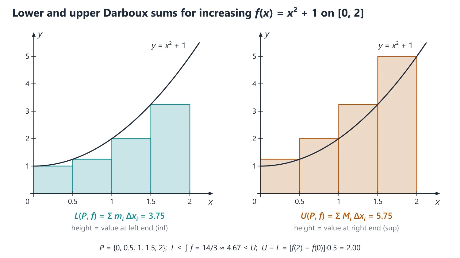
1. Understanding Upper and Lower Sums
Why we need it: 'area under a curve' needs a definition before we can prove anything about it, and some functions (such as the Dirichlet function) have no sensible area. Upper and lower sums give a definition and a test at the same time.
In words: a partition P cuts [a, b] into pieces [xi−1, xi] of lengths Δxi. On each piece, Mi is the supremum and mi the infimum of f. U(P, f) = ∑MiΔxi uses the tallest rectangle on each piece, L(P, f) = ∑miΔxi the shortest.
f is Riemann integrable when the smallest possible upper sum (the upper integral, inf U) equals the largest possible lower sum (the lower integral, sup L). Riemann's criterion says this happens iff U(P, f) − L(P, f) can be made less than any ε by a suitable P.
First example, slowly: show from the definition that ∫01 x2 dx = 1/3.
Step 1 (partition): Pn = {0, 1/n, 2/n, ..., 1}, every Δxi = 1/n.
Step 2 (sup and inf on each piece): x2 is increasing on [0, 1], so on [(i − 1)/n, i/n], Mi = i2/n2 and mi = (i − 1)2/n2.
Step 3 (sum): U = (1/n3)∑i=1n i2 = (n + 1)(2n + 1)/(6n2) and L = (1/n3)∑i=0n−1 i2 = (n − 1)(2n − 1)/(6n2).
Step 4 (squeeze): U − L = 1/n → 0, so f is integrable by Riemann's criterion; both U and L tend to 2/6 = 1/3, which is the integral. For n = 10, L = 0.285 and U = 0.385 already trap 1/3.
Non-example: f = 1 on ℚ ∩ [0, 1] and 0 elsewhere. Every piece contains rationals and irrationals, so Mi = 1 and mi = 0 for every partition: U = 1, L = 0, and U − L = 1 can never be made small. The function is bounded but not integrable.
Building up: (1) Refining P lowers U and raises L, so every lower sum is at most every upper sum (Derivation 4). (2) Hence lower integral ≤ upper integral, with equality iff U − L can be made small (Riemann's criterion).
(3) U − L = ∑(oscillation on piece i)·Δxi. A continuous f has small oscillation on short pieces (Heine–Cantor, Standard Proofs, Theorem 12); a monotone f makes the sum telescope (Theorem 16).
Where it is used: 'evaluate from the definition', 'find the upper and lower integrals' (rational/irrational functions), and limits of sums ∑(1/n)f(r/n), which are Riemann sums lying between L and U.
2. Understanding the Fundamental Theorems
Why we need it: computing integrals as limits of sums is slow. The fundamental theorems say integration and differentiation undo each other, so ∫ab f can be found from any antiderivative, and functions defined by integrals can be differentiated.
In words: first theorem: F(x) = ∫ax f(t) dt, the area accumulated up to x, is continuous, and F′(c) = f(c) at every point c where f is continuous. Second theorem: if F′ = f on [a, b] and f is integrable, then ∫ab f = F(b) − F(a).
The two hypotheses to watch are 'f continuous at c' in the first and 'f integrable' in the second; they are not automatic.
First example, slowly: find limx→0 (1/x2)∫0x t cos t dt.
Step 1 (form): at x = 0 both ∫00 t cos t dt = 0 and x2 = 0, so the quotient is 0/0.
Step 2 (differentiate the top): t cos t is continuous, so by the first fundamental theorem d/dx ∫0x t cos t dt = x cos x.
Step 3 (L'Hospital): the limit equals lim x cos x/(2x) = lim (cos x)/2 = 1/2.
Step 4 (check by the second theorem): an antiderivative of t cos t is t sin t + cos t, so the integral is x sin x + cos x − 1 ≈ x2 − x2/2 = x2/2 for small x, confirming 1/2.
Non-example: for f = [x] on [0, 2], F(x) = ∫0x [t] dt equals 0 on [0, 1] and x − 1 on [1, 2]. F is continuous, but at x = 1 its left derivative is 0 and right derivative is 1, so F′(1) does not exist: f is not continuous at 1, and the first theorem gives nothing there.
Building up: (1) |F(y) − F(x)| ≤ M|y − x| gives continuity of F. (2) (F(c + h) − F(c))/h − f(c) is the average of f(t) − f(c) over [c, c + h], which is small when f is continuous at c (Standard Proofs, Theorem 13).
(3) Second theorem: the mean value theorem writes F(b) − F(a) as a Riemann sum ∑f(ξi)Δxi, which lies between L(P, f) and U(P, f) for every P, so it equals the integral (Derivation 5). (4) Combined with the chain rule this gives the Leibniz rule for variable limits.
Where it is used: limits of ratios involving ∫0x, differentiability of F(t) = ∫0t [x] dx, integrals with a bad point such as ∫(2x sin(1/x) − cos(1/x)) dx, and differentiation under the integral sign.
3. Understanding Improper Integrals
Why we need it: the Riemann integral needs a bounded function on a bounded interval. Yet ∫0∞ e−x dx and ∫01 dx/√x clearly describe finite areas. An improper integral is defined as a limit of proper integrals.
In words: ∫a∞ f = limX→∞ ∫aX f, and if f blows up at a, ∫ab f = limε→0+ ∫a+εb f. 'Converges' means the limit exists and is finite. If there are several bad points, split the range so that each piece has one bad end, and require every piece to converge.
The yardsticks are ∫1∞ dx/xp (converges iff p > 1) and ∫01 dx/xp (converges iff p < 1). For f ≥ 0, comparison with these decides most questions.
First example, slowly: test ∫0∞ dx/(√x(1 + x2)).
Step 1 (find the bad points): the integrand is positive and continuous on (0, ∞); it blows up at 0 and the range is infinite. Split as ∫01 + ∫1∞.
Step 2 (near 0): 1 + x2 → 1, so the integrand behaves like 1/x1/2; p = 1/2 < 1, so ∫01 converges (μ-test with μ = 1/2: x1/2f(x) → 1).
Step 3 (near ∞): the integrand behaves like 1/(x1/2x2) = 1/x5/2; p = 5/2 > 1, so ∫1∞ converges (x5/2f(x) → 1).
Step 4 (conclude): both pieces converge, so the integral converges (its value is π/√2, by the substitution x = t2 and a standard integral).
Non-example: ∫0∞ dx/xp diverges for every p: near 0 it needs p < 1 and near ∞ it needs p > 1, which cannot both hold. Each piece must converge on its own.
Building up: (1) For f ≥ 0 the function X ↦ ∫aX f is increasing, so the integral converges iff it is bounded, exactly as for positive series. (2) Comparison and the μ-test follow (Why it works, above).
(3) For oscillating integrands, ∫|f| < ∞ gives absolute convergence; otherwise Dirichlet's test (bounded ∫aX f times a factor decreasing to 0) may give conditional convergence, as for ∫(sin x)/x. (4) Γ and B are improper integrals whose convergence follows from these tests (Derivation 6).
Where it is used: 'test the convergence of ∫...' questions (often with two bad points), Beta–Gamma evaluations, Laplace transforms in the ODE chapter and real integrals evaluated by residues in Complex Analysis.
4. Riemann (Darboux) Integral
Sums: for a bounded f on [a, b] and a partition P = {a = x0 < x1 < ... < xn = b}, U(P, f) = ∑MiΔxi and L(P, f) = ∑miΔxi, where Mi, mi are the sup and inf of f on [xi−1, xi].
Idea: see the figure above: U(P, f) is the area of circumscribed rectangles and overestimates, L(P, f) is the area of inscribed rectangles and underestimates. Adding points to P can only lower U and raise L, so the true area, if it exists, is trapped between them.
Integral: the upper integral is infP U(P, f) and the lower integral is supP L(P, f); f ∈ R[a, b] if they are equal, and the common value is ∫ab f(x) dx.
Idea: f is integrable when the overestimates and underestimates can be squeezed together. Boundedness is part of the definition, because otherwise some Mi or mi is infinite; unbounded integrands are handled as improper integrals.
Riemann's criterion: a bounded f is integrable iff for every ε > 0 there is a partition P with U(P, f) − L(P, f) < ε.
Integrable classes: continuous functions; monotone functions; bounded functions with finitely many (or countably many) discontinuities. Lebesgue's criterion: a bounded f is integrable iff its set of discontinuities has measure zero.
Why it works: for a continuous f, uniform continuity makes every oscillation Mi − mi small once the mesh is small (Standard Proofs, Theorem 12). For a monotone f, U − L telescopes to |f(b) − f(a)|·(b − a)/n for n equal parts (Theorem 16). Finitely many jumps can be enclosed in sub-intervals of total length as small as we like, so they contribute little to U − L.
Non-integrable: the Dirichlet function on [0, 1] has U(P, f) = 1 and L(P, f) = 0 for every P.
Properties: linearity; ∫ab = ∫ac + ∫cb; if f ∈ R then |f| and f2 ∈ R, and |∫f| ≤ ∫|f|; the product of integrable functions is integrable. The converse fails: |f| may be integrable when f is not (f = 1 on ℚ, −1 elsewhere).
Limit of sums: ∫ab f = lim ∑f(ξi)Δxi as the mesh ‖P‖ → 0; this converts limits of sums into integrals.
5. Mean Value and Fundamental Theorems
First mean value theorem: if f is continuous on [a, b], then ∫ab f = f(c)(b − a) for some c ∈ [a, b]. More generally, if f is continuous and g ∈ R[a, b] does not change sign, then ∫fg = f(c)∫g.
Why it works: with m = min f and M = max f on [a, b], m(b − a) ≤ ∫ab f ≤ M(b − a). So the average value (1/(b − a))∫ab f lies between m and M, and the IVT gives c with f(c) equal to it. For the weighted form, multiply m ≤ f ≤ M by g ≥ 0 and integrate.
Second mean value theorem (Weierstrass form): if f is monotone and g ∈ R[a, b], then ∫ab fg = f(a)∫aξ g + f(b)∫ξb g for some ξ ∈ [a, b]. Bonnet's form is the special case f ≥ 0 decreasing: ∫ab fg = f(a)∫aξ g.
First fundamental theorem: if f ∈ R[a, b] and F(x) = ∫ax f(t) dt, then F is continuous on [a, b]; if f is continuous at c, then F is differentiable at c and F′(c) = f(c).
Idea: accumulated area grows at a rate equal to the current height: F(c + h) − F(c) ≈ f(c)h. Continuity of f at c is needed: for f = sgn on [−1, 1], F(x) = ∫−1x sgn t dt = |x| − 1, which is not differentiable at 0. The proof is in Standard Proofs, Theorem 13.
Second fundamental theorem: if f ∈ R[a, b] and F is differentiable on [a, b] with F′ = f, then ∫ab f(x) dx = F(b) − F(a).
Leibniz rule: d/dx ∫u(x)v(x) f(t) dt = f(v(x))v′(x) − f(u(x))u′(x), for continuous f and differentiable u, v.
Why it works: let F be an antiderivative of f (it exists by the first fundamental theorem, as f is continuous). Then ∫u(x)v(x) f = F(v(x)) − F(u(x)), and the chain rule gives F′(v)v′ − F′(u)u′ = f(v(x))v′(x) − f(u(x))u′(x).
Example 1: Evaluate ∫01 x dx from the definition.
With Pn = {i/n}, U = ∑(i/n)(1/n) = (n + 1)/(2n) and L = ∑((i − 1)/n)(1/n) = (n − 1)/(2n). U − L = 1/n → 0, so f ∈ R[0, 1] and the integral is 1/2.
Example 2: Find limn→∞ ∑r=1n n/(n2 + r2).
The sum is ∑(1/n)·1/(1 + (r/n)2), a Riemann sum of 1/(1 + x2) on [0, 1]. The limit is ∫01 dx/(1 + x2) = π/4.
Example 3: Find limx→0 (∫0x sin(t2) dt)/x3.
It is of the form 0/0; by L'Hospital and the first fundamental theorem, the limit is lim sin(x2)/(3x2) = 1/3.
6. Improper Integrals
First kind: ∫a∞ f = limb→∞ ∫ab f, when the limit exists. Second kind: if f is unbounded near a, ∫ab f = limε→0+ ∫a+εb f.
Idea: an improper integral is a limit of proper ones. A region that is infinitely long or infinitely tall can still have finite area, provided f decays fast enough at ∞ or blows up slowly enough at the singular point.
Standard integrals: ∫1∞ dx/xp converges iff p > 1; ∫01 dx/xp converges iff p < 1; ∫0∞ e−ax dx converges iff a > 0.
Why it works: for p ≠ 1, ∫1b x−p dx = (b1−p − 1)/(1 − p), which has a finite limit as b → ∞ iff p > 1; for p = 1 it is log b → ∞. Similarly ∫ε1 x−p dx = (1 − ε1−p)/(1 − p) has a finite limit as ε → 0+ iff p < 1.
μ-test at ∞ (f ≥ 0): if limx→∞ xμf(x) is finite for some μ > 1, ∫a∞ f converges; if it is non-zero (or ∞) for some μ ≤ 1, the integral diverges.
Why it works: it is limit comparison with 1/xμ. If xμf(x) → l finite, then f(x) ≤ (l + 1)/xμ for large x, and ∫dx/xμ converges for μ > 1. If xμf(x) → l > 0 (or ∞) with μ ≤ 1, then f(x) ≥ c/xμ for large x, and ∫dx/xμ diverges.
μ-test at a singular point a (f ≥ 0): if limx→a+ (x − a)μf(x) is finite for some μ < 1, ∫ab f converges; if it is non-zero (or ∞) for some μ ≥ 1, it diverges.
Absolute convergence and tests: if ∫|f| converges then ∫f converges. Dirichlet's test: if ∫aX f is bounded for all X and g decreases monotonically to 0, then ∫a∞ fg converges. Abel's test: if ∫a∞ f converges and g is monotone and bounded, then ∫a∞ fg converges.
Conditional convergence: ∫0∞ (sin x)/x dx converges (Dirichlet) to π/2 but does not converge absolutely.
Beta and Gamma functions: Γ(n) = ∫0∞ e−xxn−1 dx converges iff n > 0, with Γ(n + 1) = nΓ(n) and Γ(1/2) = √π; B(m, n) = ∫01 xm−1(1 − x)n−1 dx converges iff m, n > 0, and B(m, n) = Γ(m)Γ(n)/Γ(m + n).
Example 4: For which m does ∫0∞ xm−1/(1 + x) dx converge?
Near 0 the integrand behaves like xm−1 = 1/x1−m, which needs 1 − m < 1, so m > 0. Near ∞ it behaves like 1/x2−m, which needs 2 − m > 1, so m < 1. It converges iff 0 < m < 1.
Example 5: Evaluate ∫0∞ e−x2 dx.
Put x2 = t, dx = dt/(2√t): the integral is (1/2)∫0∞ e−tt−1/2 dt = (1/2)Γ(1/2) = √π/2.
7. Derivation: Refinement and Riemann's Criterion
Refinement: adding one point to [xi−1, xi] splits it into two parts on which the suprema are at most Mi and the infima at least mi. So for a refinement P* of P, L(P, f) ≤ L(P*, f) ≤ U(P*, f) ≤ U(P, f).
Any lower sum ≤ any upper sum: for partitions P, Q, L(P) ≤ L(P ∪ Q) ≤ U(P ∪ Q) ≤ U(Q). Taking sup over P and inf over Q, the lower integral never exceeds the upper integral.
Criterion (⇐): if U(P) − L(P) < ε, then 0 ≤ upper integral − lower integral ≤ U(P) − L(P) < ε for every ε, so they are equal.
Criterion (⇒): if both equal I, choose P1 with U(P1) < I + ε/2 and P2 with L(P2) > I − ε/2. For P = P1 ∪ P2, refinement gives U(P) − L(P) ≤ U(P1) − L(P2) < ε.
8. Derivation: Second Fundamental Theorem
Let F′ = f on [a, b] with f ∈ R[a, b], and let P be any partition. By the mean value theorem, F(xi) − F(xi−1) = f(ξi)Δxi for some ξi ∈ (xi−1, xi). Adding, F(b) − F(a) = ∑f(ξi)Δxi.
Since mi ≤ f(ξi) ≤ Mi, L(P, f) ≤ F(b) − F(a) ≤ U(P, f) for every P. The only number between all lower and all upper sums of an integrable f is ∫ab f, so F(b) − F(a) = ∫ab f.
Note: continuity of f is never used, only differentiability of F and integrability of f; this is why the theorem applies to f(x) = 2x sin(1/x) − cos(1/x) in Example 8.
9. Derivation: Convergence and Recursion of the Gamma Function
Convergence: near 0, e−xxn−1 behaves like xn−1 = 1/x1−n, which is integrable iff 1 − n < 1, i.e. n > 0. Near ∞, xn+1e−x → 0, so x2·e−xxn−1 → 0 and the μ-test with μ = 2 gives convergence for every n.
Recursion: integrating by parts, ∫0∞ e−xxn dx = [−e−xxn]0∞ + n∫0∞ e−xxn−1 dx, and the bracket is 0 for n > 0. So Γ(n + 1) = nΓ(n); with Γ(1) = 1 this gives Γ(n + 1) = n! for n ∈ ℕ.
10. Common Mistakes
Using F(b) − F(a) across a non-integrable singularity: ∫−11 dx/x2 = [−1/x]−11 = −2 is wrong (a positive integrand cannot give a negative answer); the integral diverges at 0. Always locate singular points first.
Taking a symmetric limit for ∫−∞∞: limR→∞ ∫−RR x dx = 0, but ∫−∞∞ x dx diverges; the two ends must converge separately (the symmetric limit is only the principal value).
Declaring a function non-integrable because it has infinitely many discontinuities: the 1/n step function and Thomae's function are integrable; what matters is that the discontinuities have measure zero and f is bounded.
Linking convergence of ∫a∞ f to f(x) → 0: 1/x → 0 but ∫1∞ dx/x diverges, and ∫0∞ sin(x2) dx converges although sin(x2) has no limit.
Reversing the μ-test: at ∞, convergence needs μ > 1 with a finite limit; at a finite singular point, convergence needs μ < 1. A finite non-zero limit with μ = 1 means divergence in both cases.
11. Connections
Link: the trapezoidal and Simpson's rules of Numerical Analysis are Riemann-type sums with explicit error terms, and the limit-of-sums formula is the reverse direction of the same idea.
Link: the Laplace transform ∫0∞ e−stf(t) dt (ODE chapter) is an improper integral of the first kind, and many improper integrals, such as ∫0∞ dx/(1 + x4), are evaluated by contour integration in Complex Analysis.
12. Worked Examples
Example 6: Show that f(x) = x for rational x and f(x) = 0 for irrational x is not Riemann integrable on [0, 1].
Rationals and irrationals are dense, so on every subinterval [xi−1, xi], mi = 0 and Mi = xi.
Hence L(P, f) = 0 for every P, while U(P, f) = ∑xiΔxi ≥ ∑((xi−1 + xi)/2)Δxi = ∑(xi2 − xi−12)/2 = 1/2.
So the upper integral is at least 1/2 (in fact exactly 1/2) and the lower integral is 0. They differ, so f ∉ R[0, 1]; note f is continuous only at x = 0.
Example 7: Evaluate ∫0π/2 sin4x cos2x dx using Beta and Gamma functions.
∫0π/2 sinpx cosqx dx = (1/2)B((p + 1)/2, (q + 1)/2) for p, q > −1.
With p = 4, q = 2: (1/2)B(5/2, 3/2) = (1/2)Γ(5/2)Γ(3/2)/Γ(4).
Γ(3/2) = √π/2, Γ(5/2) = (3/2)(√π/2) = 3√π/4 and Γ(4) = 3! = 6, so the value is (1/2)(3π/8)/6 = π/32.
13. Further Techniques: Oscillation, Inequalities, Parameters and Comparison
Oscillation: for a bounded f on an interval I, the oscillation is ω(f, I) = M − m, the difference of sup f and inf f on I. Then U(P, f) − L(P, f) = ∑ωiΔxi, and ω(f, I) = sup{|f(x1) − f(x2)| : x1, x2 ∈ I}.
Integral inequalities: if f, g ∈ R[a, b] and f ≤ g, then ∫f ≤ ∫g; if moreover f, g are continuous and f(c) < g(c) at some point c, then ∫f < ∫g. In particular m(b − a) ≤ ∫ab f ≤ M(b − a).
Different rules on rationals and irrationals: let g, h be continuous on [a, b], with f = g on ℚ and f = h on the irrationals. By density and continuity, on every sub-interval sup f = sup max(g, h) and inf f = inf min(g, h).
Hence the upper integral of f is ∫ab max(g, h) and the lower integral is ∫ab min(g, h); f ∈ R[a, b] iff g = h on [a, b].
Step functions with infinitely many steps: a bounded monotone function, or one whose discontinuities are 1/2, 1/3, 1/4, ..., is integrable; integrate it piece by piece, which gives an infinite series.
Antiderivatives with a bad point: if F is differentiable on [a, b] and F′ = f ∈ R[a, b], the second fundamental theorem gives ∫ab f = F(b) − F(a), even when f is discontinuous (e.g. F(x) = x2 sin(1/x), F(0) = 0).
Differentiation under the integral sign: if f and ∂f/∂α are continuous on [a, b] × [c, d], then d/dα ∫ab f(x, α) dx = ∫ab ∂f/∂α dx. On an infinite range we also need ∫a∞ ∂f/∂α dx to converge uniformly in α, e.g. through a bound |∂f/∂α| ≤ M(x) with ∫M convergent.
Comparison for improper integrals: if 0 ≤ f ≤ g, convergence of ∫g gives convergence of ∫f; in limit form, if f/g → l with 0 < l < ∞, both converge or both diverge. With two singular points (or a singular point and ∞), split the range and test each piece.
Divergence through a series: for f ≥ 0, ∫0∞ f converges iff ∑n ∫nπ(n+1)π f converges; this handles integrands such as 1/(1 + x2sin2x) that are not monotone.
14. Solved Past UPSC Questions
Example 8 (UPSC 2014, 15 marks): Integrate ∫01 f(x) dx, where
f(x) = 2x sin(1/x) − cos(1/x), x ∈ ]0, 1]
f(x) = 0, x = 0
f is bounded on [0, 1] (|f(x)| ≤ 2x + 1 ≤ 3) and continuous except at x = 0, so f ∈ R[0, 1].
Let F(x) = x2 sin(1/x) for x ≠ 0 and F(0) = 0. For 0 < x ≤ 1, F′(x) = 2x sin(1/x) − cos(1/x) = f(x).
At 0, F′(0) = limh→0+ h sin(1/h) = 0 = f(0). So F is differentiable on [0, 1] with F′ = f.
By the second fundamental theorem (F′ = f ∈ R[0, 1]), ∫01 f(x) dx = F(1) − F(0) = sin 1.
Answer: ∫01 f(x) dx = sin 1 ≈ 0.8415.
Example 9 (UPSC 2015, 15 marks): Is the function
f(x) = 1/n, 1/(n + 1) < x ≤ 1/n
f(x) = 0, x = 0
Riemann integrable? If yes, obtain the value of ∫01 f(x) dx.
f is bounded (0 ≤ f ≤ 1) and increasing on [0, 1]: a larger x lies in an interval (1/(n + 1), 1/n] with smaller n, hence larger value 1/n.
A monotone function is Riemann integrable, so f ∈ R[0, 1] (alternatively, its discontinuities 1/2, 1/3, ... form a countable set).
Since 0 ≤ ∫0c f ≤ c, ∫01 f = limc→0+ ∫c1 f, and on each piece (1/(n + 1), 1/n] f is the constant 1/n.
So ∫01 f = ∑n=1∞ (1/n)(1/n − 1/(n + 1)) = ∑ 1/(n2(n + 1)).
1/(n2(n + 1)) = 1/n2 − 1/n + 1/(n + 1), and ∑(1/(n + 1) − 1/n) = −1 (telescoping), so the sum is π2/6 − 1.
Answer: yes, f is Riemann integrable and ∫01 f(x) dx = π2/6 − 1 ≈ 0.645.
Example 10 (UPSC 2017, 15 marks): Let f(t) = ∫0t [x] dx, where [x] denotes the largest integer less than or equal to x.
(i) Determine all the real numbers t at which f is differentiable.
(ii) Determine all the real numbers t at which f is continuous but not differentiable.
[x] is bounded on bounded intervals and continuous except at the integers, so f(t) = ∫0t [x] dx is defined for every real t (for t < 0 it means −∫t0 [x] dx).
By the first fundamental theorem f is continuous on ℝ, and f′(t) = [t] at every t where [x] is continuous, i.e. at every t ∉ ℤ.
At an integer n: for n ≤ t < n + 1, f(t) = f(n) + n(t − n), so the right derivative is n; for n − 1 ≤ t < n, f(t) = f(n) − (n − 1)(n − t), so the left derivative is n − 1.
The one-sided derivatives differ, so f is not differentiable at any integer.
Answer: (i) f is differentiable exactly at t ∈ ℝ∖ℤ, with f′(t) = [t]; (ii) f is continuous everywhere, so it is continuous but not differentiable exactly at the integers.
Example 11 (UPSC 2018, 10 marks): Prove the inequality : π2/9 < ∫π/6π/2 (x/sin x) dx < 2π2/9.
On [π/6, π/2], 1/2 ≤ sin x ≤ 1, so x ≤ x/sin x ≤ 2x.
sin x < 1 for x < π/2 and sin x > 1/2 for x > π/6, so each inequality is strict except at one end point; the functions are continuous, so the integrated inequalities are strict.
∫π/6π/2 x dx = (1/2)(π2/4 − π2/36) = π2/9, and ∫π/6π/2 2x dx = 2π2/9.
Answer: π2/9 < ∫π/6π/2 (x/sin x) dx < 2π2/9 (numerically 1.097 < 1.300 < 2.193).
Example 12 (UPSC 2019, 10 marks): Evaluate
∫0∞ tan−1(ax)/(x(1 + x2)) dx, a > 0, a ≠ 1.
Let I(a) = ∫0∞ tan−1(ax)/(x(1 + x2)) dx, a ≥ 0. The integrand is continuous on (0, ∞), tends to a as x → 0 and is at most π/(2x(1 + x2)), so I(a) converges, and I(0) = 0.
∂/∂a of the integrand is 1/((1 + a2x2)(1 + x2)) ≤ 1/(1 + x2), whose integral converges; so the differentiated integral converges uniformly for a ≥ 0 and we may differentiate under the integral sign.
For a ≠ 1, 1/((1 + a2x2)(1 + x2)) = (1/(1 − a2))[1/(1 + x2) − a2/(1 + a2x2)].
Since ∫0∞ a dx/(1 + a2x2) = π/2 for a > 0, I′(a) = (1/(1 − a2))(π/2 − aπ/2) = π/(2(1 + a)).
Integrating, I(a) = (π/2) log(1 + a) + C, and I(0) = 0 gives C = 0.
Answer: ∫0∞ tan−1(ax)/(x(1 + x2)) dx = (π/2) loge(1 + a) (checked numerically: a = 2 gives 1.7257).
Example 13 (UPSC 2020, 15 marks): Show that ∫0π/2 sin2x/(sin x + cos x) dx = (1/√2) loge(1 + √2)
Let I be the integral. The substitution x → π/2 − x gives I = ∫0π/2 cos2x/(cos x + sin x) dx.
Adding, 2I = ∫0π/2 dx/(sin x + cos x) = (1/√2)∫0π/2 dx/sin(x + π/4).
Using ∫cosec θ dθ = log tan(θ/2), 2I = (1/√2)[log tan(3π/8) − log tan(π/8)].
tan(3π/8) = √2 + 1 and tan(π/8) = √2 − 1, so 2I = (1/√2) log((√2 + 1)/(√2 − 1)) = (1/√2) log(√2 + 1)2 = √2 log(1 + √2).
Answer: I = (1/√2) loge(1 + √2) ≈ 0.6232, as required.
Example 14 (UPSC 2023, 15 marks): Prove that the oscillation of a real-valued bounded function f defined on [a, b] is the supremum of the set {|f(x1) − f(x2)| : x1, x2 ∈ [a, b]}.
Let M = sup f and m = inf f on [a, b], so the oscillation is M − m, and let S = {|f(x1) − f(x2)| : x1, x2 ∈ [a, b]}, a bounded set.
For all x1, x2, m ≤ f(x1), f(x2) ≤ M, so |f(x1) − f(x2)| ≤ M − m: M − m is an upper bound of S.
Let ε > 0. By the definitions of sup and inf there are x1, x2 with f(x1) > M − ε/2 and f(x2) < m + ε/2.
Then |f(x1) − f(x2)| ≥ f(x1) − f(x2) > M − m − ε, so no number less than M − m is an upper bound of S.
Answer: sup S = M − m, the oscillation of f on [a, b].
Example 15 (UPSC 2024, 10 marks): Test the convergence of ∫02 log x/√(2 − x) dx.
The integrand has two singular points, x = 0 (log x → −∞) and x = 2 (the denominator vanishes). Split the integral at 1.
On (0, 1] the integrand is ≤ 0; take g(x) = −log x/√(2 − x) ≥ 0. With μ = 1/2, xμg(x) = −√x log x/√(2 − x) → 0 as x → 0+, a finite limit with μ < 1, so ∫01 converges.
On [1, 2) the integrand is ≥ 0, and with μ = 1/2, (2 − x)μ·log x/√(2 − x) = log x → log 2 as x → 2−, finite with μ < 1, so ∫12 converges.
Answer: ∫02 log x/√(2 − x) dx is convergent.
Example 16 (UPSC 2024, 15 marks): Find the upper and lower Riemann integrals for the function f defined on [0, 1] as follows:
f(x) = (1 − x2)1/2, if x is rational.
f(x) = (1 − x), if x is irrational.
Hence, show that f is not Riemann integrable on [0, 1].
Let g(x) = √(1 − x2) and h(x) = 1 − x, continuous on [0, 1]. Since (1 − x2) − (1 − x)2 = 2x(1 − x) ≥ 0, g ≥ h on [0, 1], with equality only at 0 and 1.
On each sub-interval J of a partition, rationals and irrationals are dense, so supJ f = supJ g and infJ f = infJ h.
Hence U(P, f) = U(P, g) and L(P, f) = L(P, h) for every P, so the upper integral is ∫01 √(1 − x2) dx = π/4 (a quarter of the unit disc) and the lower integral is ∫01 (1 − x) dx = 1/2.
π/4 ≈ 0.785 ≠ 1/2, so f is not Riemann integrable on [0, 1].
Answer: upper integral π/4, lower integral 1/2; f ∉ R[0, 1].
Example 17 (UPSC 2026, 20 marks): A function f is defined on [0, 1] by
f(x) = x2, when x is rational;
f(x) = x3, when x is irrational.
Evaluate the lower integral ∫01 f and the upper integral ∫01 f. Does the integral ∫01 f exist?
On [0, 1], x3 ≤ x2, with equality only at 0 and 1; both functions are continuous.
By density, on every sub-interval sup f = sup x2 and inf f = inf x3, so U(P, f) = U(P, x2) and L(P, f) = L(P, x3) for every partition P.
Hence the upper integral is ∫01 x2 dx = 1/3 and the lower integral is ∫01 x3 dx = 1/4.
Answer: lower integral 1/4, upper integral 1/3; since they differ, ∫01 f does not exist.
Example 18 (UPSC 2026, 15 marks): Prove that the improper integral ∫0∞ dx/(1 + x2 sin2x) is divergent.
f(x) = 1/(1 + x2sin2x) > 0, so ∫0∞ f converges iff ∑n≥0 In converges, where In = ∫nπ(n+1)π f(x) dx.
On [nπ, (n + 1)π], x ≤ (n + 1)π, and with x = nπ + t, sin2x = sin2t. So In ≥ ∫0π dt/(1 + A sin2t) with A = (n + 1)2π2.
∫0π dt/(1 + A sin2t) = 2∫0π/2 sec2t dt/(1 + (1 + A)tan2t) = π/√(1 + A) (put u = tan t).
Hence In ≥ π/√(1 + (n + 1)2π2) ≥ π/√(2(n + 1)2π2) = 1/(√2(n + 1)), since 1 ≤ (n + 1)2π2.
∑1/(n + 1) diverges, so ∑In diverges by comparison. (Note that the integrand does not tend to 0: it equals 1 at every x = nπ.)
Answer: ∫0∞ dx/(1 + x2sin2x) diverges.
15. Practice Exercises
Exercise 1 (basic): For f(x) = x2 on [0, 1] and P = {0, 1/2, 1}, compute U(P, f) and L(P, f).
Answer: U = (1/4 + 1)(1/2) = 5/8 and L = (0 + 1/4)(1/2) = 1/8.
Exercise 2 (basic): Is f(x) = 1/x for 0 < x ≤ 1, f(0) = 0, Riemann integrable on [0, 1]?
Answer: no: it is unbounded, so the first piece of every partition has M1 = ∞ (and ∫01 dx/x also diverges as an improper integral).
Exercise 3 (basic): Find d/dx ∫0x2 cos(t2) dt.
Answer: 2x cos(x4), by the first fundamental theorem and the chain rule.
Exercise 4 (standard): Evaluate limn→∞ ∑r=1n 1/(n + r).
Answer: ∑(1/n)·1/(1 + r/n) → ∫01 dx/(1 + x) = log 2.
Exercise 5 (standard): Evaluate limn→∞ (12 + 22 + ... + n2)/n3 as an integral.
Answer: ∑(1/n)(r/n)2 → ∫01 x2 dx = 1/3.
Exercise 6 (standard): Test ∫0∞ dx/(√x(1 + x)) and find its value.
Answer: near 0 it behaves like x−1/2 and near ∞ like x−3/2, so it converges; x = t2 gives 2∫0∞ dt/(1 + t2) = π.
Exercise 7 (standard): Show that ∫01 log x dx converges and find its value.
Answer: ∫ε1 log x dx = [x log x − x]ε1 = −1 − ε log ε + ε → −1, since ε log ε → 0.
Exercise 8 (standard): Evaluate ∫01 x3(1 − x)4 dx using the Beta function.
Answer: B(4, 5) = Γ(4)Γ(5)/Γ(9) = 3!·4!/8! = 1/280.
Exercise 9 (UPSC level): For p > 0, discuss the absolute and conditional convergence of ∫1∞ (sin x)/xp dx.
Answer: for p > 1, |sin x|/xp ≤ 1/xp: absolutely convergent. For 0 < p ≤ 1, Dirichlet's test (|∫1X sin x dx| ≤ 2, 1/xp decreasing to 0) gives convergence, while |sin x| ≥ sin2x = (1 − cos 2x)/2 shows ∫|sin x|/xp diverges: conditionally convergent.
Exercise 10 (UPSC level): Using differentiation under the integral sign, show that ∫0∞ e−ax(sin x)/x dx = tan−1(1/a) for a > 0.
Answer: I′(a) = −∫0∞ e−ax sin x dx = −1/(1 + a2) (uniform for a ≥ a0 > 0), and I(a) → 0 as a → ∞, so I(a) = π/2 − tan−1a = tan−1(1/a).
Exercise 11 (UPSC level): Let f(x) = 2x for rational x and f(x) = x2 for irrational x, on [0, 1]. Find the upper and lower integrals. Is f integrable?
Answer: 2x − x2 = x(2 − x) ≥ 0 on [0, 1], so the upper integral is ∫01 2x dx = 1 and the lower integral is ∫01 x2 dx = 1/3; they differ, so f is not integrable.
| Integral | Converges iff | Value (when convergent) |
|---|---|---|
| ∫1∞ dx/xp | p > 1 | 1/(p − 1) |
| ∫01 dx/xp | p < 1 | 1/(1 − p) |
| ∫0∞ e−xxn−1 dx | n > 0 | Γ(n) |
| ∫01 xm−1(1 − x)n−1 dx | m > 0, n > 0 | B(m, n) = Γ(m)Γ(n)/Γ(m + n) |
| ∫0∞ (sin x)/x dx | always (conditionally) | π/2 |
| ∫0∞ xm−1/(1 + x) dx | 0 < m < 1 | π/sin(mπ) |
| Form of the problem | Method | Watch out for |
|---|---|---|
| Is a given bounded f integrable? | Continuous, monotone, or discontinuities of measure zero; else Riemann's criterion | Unbounded f is never Riemann integrable |
| f has different rules on ℚ and on the irrationals | Upper integral = ∫max(g, h), lower = ∫min(g, h) | Integrable iff g = h |
| limn→∞ (1/n)∑f(r/n) | Recognise a Riemann sum of f on [0, 1] | Bring the sum to the form ∑f(r/n)·(1/n) |
| Limit involving ∫0x f(t) dt | First fundamental theorem + L'Hospital | Needs f continuous at the point |
| ∫ab f with F′ = f known | Second fundamental theorem | F′ = f must hold on all of [a, b] and f ∈ R[a, b] |
| Improper, f ≥ 0 | Comparison or μ-test at each singular point | Split the range at every singular point |
| Improper, oscillating integrand | Dirichlet or Abel test; absolute convergence separately | Conditional convergence is possible |
| Integral with a parameter | Differentiate under the integral sign, then integrate in the parameter | Justify the interchange (continuity or uniform convergence) |
| Inequality for ∫f | Bound f between m and M, or compare integrands | Strict inequality needs f, g continuous and f ≠ g somewhere |
Mains points
- Typical questions: prove a given function (for example one with finitely many discontinuities, or [x] on an interval) is Riemann integrable and evaluate the integral via upper and lower sums.
- Limits of sums such as ∑n/(n2 + r2) or ∑1/(n + r) are converted to definite integrals; show the 1/n factor and the variable r/n clearly.
- For improper integrals, split at every singular point and at ∞, test each piece separately, and name the comparison function; this structure earns full marks.
- State both fundamental theorems with hypotheses; note that the second theorem needs f ∈ R[a, b], not just the existence of an antiderivative.
- Common mistake: treating ∫−11 dx/x2 as a proper integral and getting −2; check the integrand for singularities first.
Did you know?
- Riemann defined his integral in 1854 in a paper on trigonometric series, and Darboux later recast it with upper and lower sums, the form used in most examinations.
Uniform Convergence of Sequences and Series of Functions
A sequence of functions converges uniformly when sup|fn − f| → 0, so a single N works for every x. Uniform convergence preserves continuity and allows term-by-term integration; term-by-term differentiation needs uniform convergence of the derivatives. The Weierstrass M-test is the standard tool for series.
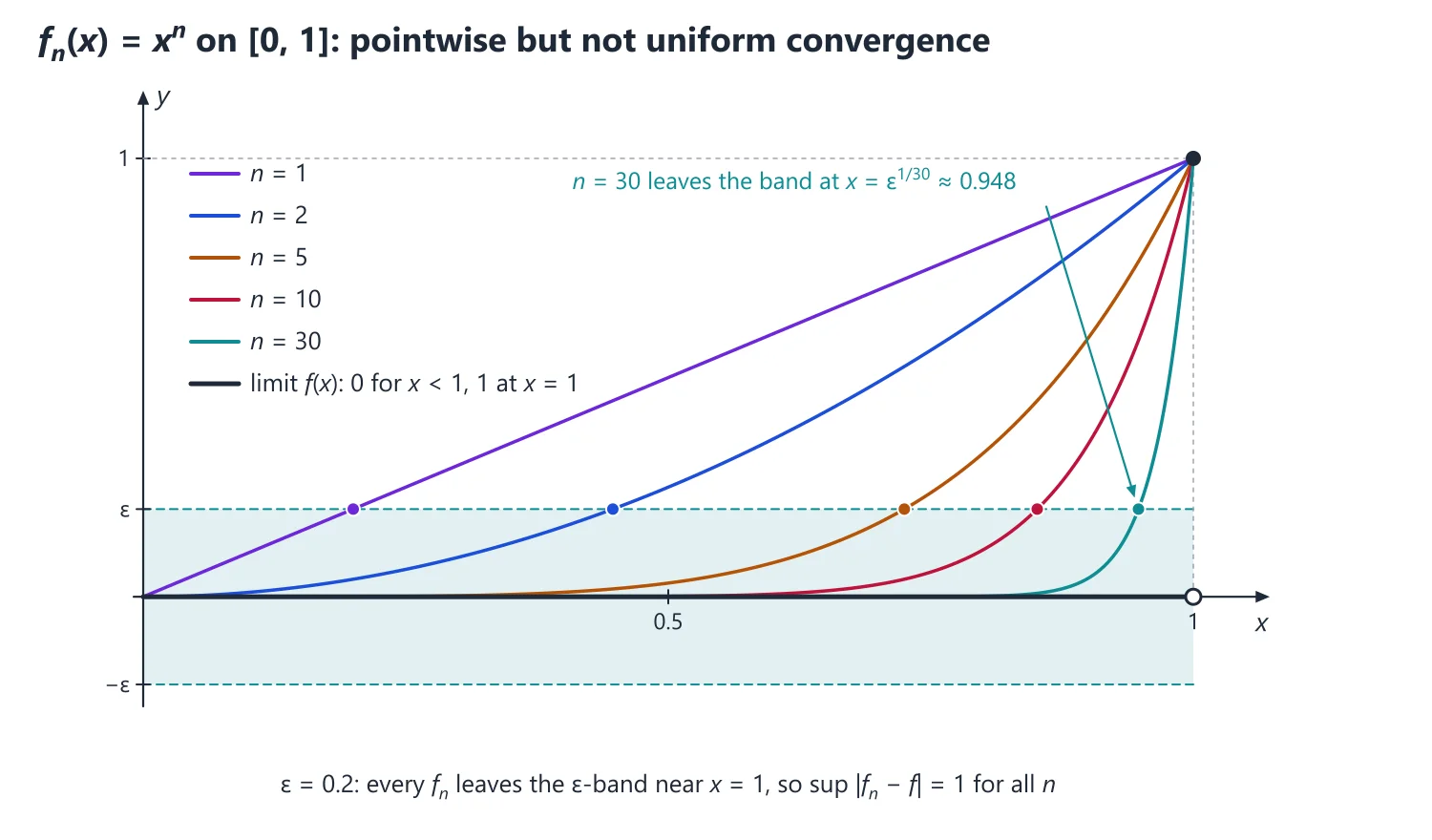
1. Understanding Pointwise and Uniform Convergence
Why we need it: functions are often built as limits, for example sums of power series or Fourier series. We want the limit to inherit good properties (continuity, integrals, derivatives). Pointwise convergence is too weak for this: each fn(x) = xn is continuous on [0, 1], but the limit jumps at x = 1.
In words: pointwise: fix x first; then the numbers fn(x) converge to f(x), with an N that may depend on x. Uniform: for every ε one N works for all x in E at once, i.e. supx∈E |fn(x) − f(x)| → 0.
The number Mn = supx∈E |fn(x) − f(x)| is the worst error of fn over the whole set. Uniform convergence means the worst error tends to 0; pointwise means only that each individual error does.
First example, slowly: fn(x) = x/(1 + nx) on [0, ∞).
Step 1 (pointwise limit): fn(0) = 0; for fixed x > 0, x/(1 + nx) ≤ x/(nx) = 1/n → 0. So f = 0.
Step 2 (the worst error): Mn = supx≥0 x/(1 + nx). The function x/(1 + nx) increases with x (its derivative is 1/(1 + nx)2 > 0) and tends to 1/n as x → ∞, so Mn = 1/n.
Step 3 (decide): Mn = 1/n → 0, so the convergence is uniform on [0, ∞). Given ε, N > 1/ε works for every x simultaneously.
Step 4 (contrast): for gn(x) = nx/(1 + nx) the pointwise limit is 1 for x > 0 and 0 at x = 0; it is discontinuous, so the convergence of these continuous gn cannot be uniform on [0, ∞).
Non-example: fn(x) = xn on [0, 1) converges to 0 at every point, but Mn = sup[0, 1) xn = 1 for every n (take x close to 1). The worst error never shrinks, so the convergence is pointwise but not uniform, even though the limit 0 is continuous.
Building up: (1) The Mn-test is just the definition rewritten with a supremum. (2) To compute Mn, maximise |fn − f| by calculus and check the end points (Derivation 5). (3) To disprove uniformity it is enough to find one xn per n with |fn(xn) − f(xn)| ≥ ε0.
(4) The answer depends on the set: xn converges uniformly on [0, a] for a < 1 (Mn = an) but not on [0, 1). Always state the set on which you claim uniformity.
Where it is used: the most common UPSC question in this topic: 'test fn(x) = ... for uniform convergence on ...'; also the starting point of every theorem on continuity, integration and differentiation of limits.
2. Understanding the Weierstrass M-test
Why we need it: for a series ∑un(x) we usually cannot write the sum S(x), so we cannot compute sup|Sn − S|. We need a test that uses only the individual terms.
In words: find numbers Mn (constants, not depending on x) such that |un(x)| ≤ Mn for every x ∈ E and every n. If the number series ∑Mn converges, then ∑un(x) converges uniformly and absolutely on E.
The best choice is Mn = supx∈E |un(x)|, found by calculus or by a simple inequality; any larger constant also works if its series still converges.
First example, slowly: show that ∑n=1∞ cos(nx)/(n2 + x2) converges uniformly on ℝ.
Step 1 (bound the numerator): |cos(nx)| ≤ 1 for all x.
Step 2 (bound the denominator from below): n2 + x2 ≥ n2 for all x.
Step 3 (combine): |un(x)| ≤ 1/n2 = Mn, a number independent of x.
Step 4 (conclude): ∑1/n2 converges, so the series converges uniformly (and absolutely) on ℝ by the M-test. Each term is continuous, so the sum is a continuous function on ℝ.
Non-example: for ∑xn on (−1, 1), sup|xn| = 1, so the best Mn is 1 and ∑1 diverges: the M-test fails, and indeed the convergence is not uniform on (−1, 1) (the tail xn/(1 − x) is unbounded near 1). On [−r, r] with r < 1, Mn = rn works.
Building up: (1) The tail of the function series is at most the tail of ∑Mn: |un+1(x) + ... + um(x)| ≤ Mn+1 + ... + Mm, with no x on the right. (2) The Cauchy criterion for uniform convergence then applies (Standard Proofs, Theorem 15).
(3) The M-test proves absolute and uniform convergence together, so it cannot handle series that converge only conditionally, such as ∑(−1)n/(n + x2); for those use Dirichlet's or Abel's uniform tests.
Where it is used: the first tool for any series of functions; power series on [−r, r]; Fourier series with ∑|an| < ∞; justifying term-by-term differentiation when applied to the derived series.
3. Understanding What Uniform Convergence Preserves
Why we need it: in exams we are asked whether lim ∫fn = ∫lim fn, whether the sum of a series is continuous, or whether a series can be differentiated term by term. These are interchanges of two limiting processes, and they can fail.
In words: (i) uniform limit of continuous functions is continuous; (ii) on a bounded interval, a uniform limit of integrable functions is integrable and ∫fn → ∫f; (iii) if fn′ converge uniformly and fn(x0) converges at one point, then (lim fn)′ = lim fn′.
Notice that in (iii) the hypothesis is on the derivatives, not on the functions. All three are sufficient conditions; when they fail, the conclusion may still hold and must be checked directly.
First example, slowly: decide whether lim ∫01 fn = ∫01 lim fn for fn(x) = 2n2x e−n2x2.
Step 1 (pointwise limit): fn(0) = 0, and for fixed x > 0 the exponential e−n2x2 beats the factor 2n2, so fn(x) → 0. Thus ∫01 lim fn = 0.
Step 2 (integrate first): ∫01 2n2x e−n2x2 dx = [−e−n2x2]01 = 1 − e−n2 → 1.
Step 3 (compare): 1 ≠ 0, so the interchange fails. By theorem (ii), the convergence cannot be uniform on [0, 1].
Step 4 (confirm with Mn): fn is largest at x = 1/(n√2), where it equals n√2·e−1/2 → ∞. The mass of fn is a spike of area about 1 squeezed towards 0: pointwise it vanishes, but its area does not.
Non-example: fn(x) = sin(n2x)/n → 0 uniformly on ℝ (Mn = 1/n), but fn′(x) = n cos(n2x) does not converge (at x = 0 it equals n). Uniform convergence of the functions does not allow term-by-term differentiation; the derivative condition in (iii) fails.
Building up: (1) Continuity: the ε/3 argument (Standard Proofs, Theorem 14). (2) Integration: |∫fn − ∫f| ≤ (b − a)Mn → 0 (Derivation 6). (3) Differentiation: apply (ii) to fn′ to get fn(x) − fn(x0) = ∫x0x fn′ → ∫x0x g, then the fundamental theorem gives f′ = g (when the fn′ are continuous).
(4) Contrapositives are the quick tools: a discontinuous limit of continuous functions, or lim ∫fn ≠ ∫lim fn on a bounded interval, proves that the convergence is not uniform.
Where it is used: 'can the series be integrated or differentiated term by term?' questions; continuity of sums of series; in PDE, checking that Fourier-series solutions really satisfy the equation.
4. Understanding Power Series and the Radius of Convergence
Why we need it: functions such as ex, sin x and log(1 + x) are given by power series ∑anxn. We must know for which x such a series converges, and whether we may differentiate or integrate it term by term.
In words: there is a number R, 0 ≤ R ≤ ∞, the radius of convergence, such that the series converges absolutely for |x| < R and diverges for |x| > R. It is given by 1/R = lim sup |an|1/n, or 1/R = lim |an+1/an| when this limit exists. At x = ±R anything can happen.
Inside, on every closed interval [−r, r] with r < R, the convergence is uniform, so the sum is continuous and can be differentiated and integrated term by term on (−R, R).
First example, slowly: find where ∑n=1∞ xn/(n·2n) converges.
Step 1 (coefficients): an = 1/(n·2n), so |an+1/an| = n/(2(n + 1)) → 1/2. Hence R = 2.
Step 2 (inside and outside): absolute convergence for |x| < 2, divergence for |x| > 2 (the terms do not tend to 0).
Step 3 (end point x = 2): the series becomes ∑1/n, which diverges.
Step 4 (end point x = −2): it becomes ∑(−1)n/n, which converges by Leibniz but not absolutely. So the interval of convergence is [−2, 2), and the sum is −log(1 − x/2) there.
Non-example: for ∑n!xn, |an+1/an| = n + 1 → ∞, so R = 0: the series converges only at x = 0. Having a formula with powers of x does not guarantee convergence anywhere else.
Building up: (1) Root test on |anxn| gives the radius (Cauchy–Hadamard, Derivation 7). (2) On [−r, r], |anxn| ≤ |an|rn, a convergent number series: the M-test gives uniformity.
(3) The derived series ∑nanxn−1 has the same radius, so term-by-term differentiation is valid inside. (4) If the series converges at x = R, Abel's limit theorem makes the sum continuous up to R; this is how log 2 = 1 − 1/2 + 1/3 − ... is proved.
Where it is used: radius and interval of convergence questions; summing series by differentiating or integrating a geometric series; Taylor and Laurent series in Complex Analysis; series solutions of ODEs.
5. Pointwise and Uniform Convergence
Pointwise: fn → f on E if fn(x) → f(x) for each x ∈ E; here N may depend on both ε and x.
Idea: pointwise convergence lets every x converge at its own speed. For xn on [0, 1), the point x = 0.5 needs about 7 terms to get within 0.01 of 0, while x = 0.99 needs about 459; no single N serves all x.
Uniform: fn → f uniformly on E if for every ε > 0 there is N, depending only on ε, with |fn(x) − f(x)| < ε for all n ≥ N and all x ∈ E.
Idea: see the figure above: uniform convergence means that, for n ≥ N, the whole graph of fn lies inside the band of half-width ε around the graph of f. For xn on [0, 1] each graph climbs from near 0 to 1 close to x = 1, so it always leaves the band; on [0, a] with a < 1 it stays inside eventually.
Mn-test: fn → f uniformly on E iff Mn = supx∈E |fn(x) − f(x)| → 0.
Cauchy criterion: (fn) converges uniformly on E iff for every ε > 0 there is N with |fm(x) − fn(x)| < ε for all m, n ≥ N and all x ∈ E.
Use: like the Cauchy criterion for numbers, it proves uniform convergence when the limit function is unknown, which is the usual situation for a series ∑un(x); applied to partial sums it reads |un+1(x) + ... + um(x)| < ε for all x ∈ E and m > n ≥ N.
Example 1: fn(x) = xn on [0, 1].
The pointwise limit is 0 for 0 ≤ x < 1 and 1 at x = 1. The limit is discontinuous while each fn is continuous, so the convergence is not uniform on [0, 1]. On [0, a] with a < 1, Mn = an → 0, so it is uniform there.
Example 2: fn(x) = nx/(1 + n2x2) on [0, 1].
The pointwise limit is 0. The maximum of fn is at x = 1/n, where fn = 1/2, so Mn = 1/2 does not tend to 0; the convergence is not uniform, although the limit is continuous.
6. Tests for Series of Functions
Weierstrass M-test: if |un(x)| ≤ Mn for all x ∈ E and ∑Mn converges, then ∑un(x) converges uniformly and absolutely on E.
Idea: dominate every term by a number, uniformly in x; then the tail of ∑un(x) is at most the tail of ∑Mn, which does not depend on x (Standard Proofs, Theorem 15). The test gives absolute and uniform convergence together, so it cannot handle series that converge only conditionally.
Dirichlet's test: if the partial sums of ∑an(x) are uniformly bounded on E and bn(x) is monotone in n for each x and tends to 0 uniformly, then ∑an(x)bn(x) converges uniformly on E.
Abel's test: if ∑an(x) converges uniformly on E and bn(x) is monotone in n for each x and uniformly bounded, then ∑an(x)bn(x) converges uniformly on E.
Example 3: ∑sin(nx)/n2 converges uniformly on ℝ, since |sin(nx)/n2| ≤ 1/n2 and ∑1/n2 converges.
7. Continuity, Integrability and Differentiability
Continuity: if each fn is continuous on E and fn → f uniformly on E, then f is continuous on E. So a sum of a uniformly convergent series of continuous functions is continuous.
Idea: the ε/3 argument: |f(x) − f(c)| ≤ |f(x) − fN(x)| + |fN(x) − fN(c)| + |fN(c) − f(c)|, where uniformity controls the outer terms for all x at once and continuity of fN controls the middle one (Standard Proofs, Theorem 14). Its contrapositive is the quickest test: a discontinuous limit of continuous functions means the convergence is not uniform.
Dini's theorem: if E is compact, fn are continuous, fn(x) is monotone in n for each x, and the pointwise limit f is continuous, then the convergence is uniform.
Why each hypothesis is needed: on [0, 1), xn decreases to the continuous limit 0 but not uniformly (the domain is not compact); on [0, 1], xn is monotone but its limit is discontinuous; and nx/(1 + n2x2) on [0, 1] has a continuous limit on a compact set but is not monotone in n, and the convergence is not uniform.
Integration: if fn ∈ R[a, b] and fn → f uniformly on [a, b], then f ∈ R[a, b] and ∫ab fn → ∫ab f; a uniformly convergent series of integrable functions may be integrated term by term.
Differentiation: if each fn is differentiable on [a, b], (fn(x0)) converges for some x0 ∈ [a, b], and (fn′) converges uniformly on [a, b], then (fn) converges uniformly to some f, f is differentiable, and f′ = lim fn′.
Idea: derivatives are sensitive to small fast wiggles. sin(nx)/√n is uniformly within 1/√n of 0, yet its slope √n cos(nx) grows without bound. That is why the hypothesis is placed on the derivatives (fn′ converge uniformly), not on the functions.
Uniform convergence is sufficient, not necessary: xn on [0, 1] does not converge uniformly, yet ∫01 xn dx = 1/(n + 1) → 0 = ∫01 f.
Term-by-term differentiation without uniformity: lim fn′ = (lim fn)′ can hold even when (fn′) is not uniformly convergent, since that condition is only sufficient. To test a given series, compute S(x) = lim Sn(x) and lim Sn′(x) directly and compare.
Check pointwise convergence first: a series ∑un(x) that diverges at some points (e.g. because un(x) behaves like c/n there) cannot converge uniformly on any set containing those points.
Weierstrass approximation theorem: every continuous function on [a, b] is the uniform limit on [a, b] of a sequence of polynomials.
Idea: polynomials are dense among continuous functions on [a, b]: any continuous graph, however irregular, can be followed within any ε by a single polynomial. On an unbounded interval this fails, since a non-constant polynomial is unbounded on ℝ while sin x is bounded.
Failure of integration: fn(x) = n2x e−nx on [0, 1] tends to 0 pointwise, but ∫01 fn = 1 − (n + 1)e−n → 1 ≠ 0.
Failure of differentiation: fn(x) = sin(nx)/√n → 0 uniformly on ℝ, but fn′(x) = √n cos(nx) does not converge (at x = 0 it equals √n).
8. Power Series
Radius of convergence: for ∑anxn, 1/R = lim sup |an|1/n (or lim |an+1/an| when it exists). The series converges absolutely for |x| < R and diverges for |x| > R.
Uniformity: a power series converges uniformly on [−r, r] for every r < R, so its sum is continuous on (−R, R) and can be differentiated and integrated term by term there.
Abel's limit theorem: if ∑anRn converges, then the series converges uniformly on [0, R] and its sum is continuous at x = R from the left; for example log 2 = 1 − 1/2 + 1/3 − ....
Example 4: Show that ∑x/((1 + (n − 1)x)(1 + nx)) does not converge uniformly on [0, 1].
The terms telescope: x/((1 + (n − 1)x)(1 + nx)) = 1/(1 + (n − 1)x) − 1/(1 + nx), so Sn(x) = 1 − 1/(1 + nx). The sum is 1 for x > 0 and 0 at x = 0, which is discontinuous, so the convergence cannot be uniform on [0, 1].
9. Derivation: Computing Mn in Practice
Steps: (1) find the pointwise limit f; (2) put gn(x) = |fn(x) − f(x)|; (3) maximise gn on E using gn′ = 0 and the end points; (4) decide whether Mn → 0.
Illustration: for fn(x) = xn(1 − x) on [0, 1], f = 0, and fn′(x) = xn−1(n − (n + 1)x) = 0 at x = n/(n + 1). So Mn = (n/(n + 1))n·1/(n + 1) ≤ 1/(n + 1) → 0, and the convergence is uniform on [0, 1], although xn alone does not converge uniformly there.
Disproving uniformity quickly: one point xn per n with |fn(xn) − f(xn)| ≥ ε0 is enough, since then Mn ≥ ε0. For nx/(1 + n2x2) take xn = 1/n, where the value is 1/2.
10. Derivation: Term-by-Term Integration
If fn → f uniformly on [a, b] and all are integrable, then |∫ab fn − ∫ab f| ≤ ∫ab |fn − f| ≤ (b − a)Mn → 0.
Applied to the partial sums Sn of a uniformly convergent series this gives ∫∑un = ∑∫un. The factor (b − a) is why the argument needs a bounded interval: on [0, ∞), fn = (1/n)·(indicator of [0, n]) tends to 0 uniformly, but ∫0∞ fn = 1 for every n.
11. Derivation: Radius of Convergence and Uniformity of Power Series
Cauchy–Hadamard: apply the root test to ∑|anxn|: lim sup |anxn|1/n = |x|·lim sup |an|1/n = |x|/R. It is less than 1 for |x| < R (absolute convergence) and greater than 1 for |x| > R (terms do not tend to 0).
Uniform on [−r, r], r < R: |anxn| ≤ |an|rn = Mn, and ∑Mn converges because r < R; the M-test applies.
Derived series: ∑nanxn−1 has the same radius, because n1/n → 1 leaves the lim sup unchanged. So the derived series also converges uniformly on [−r, r], and the differentiation theorem justifies (∑anxn)′ = ∑nanxn−1 on (−R, R).
12. Choosing the Method
If a sequence (fn) is given → find f; if the fn are continuous and f is not, stop: not uniform. Otherwise compute Mn by calculus.
If a series has |un(x)| ≤ Mn with ∑Mn convergent → Weierstrass M-test; find Mn as supx|un(x)|.
If a series has oscillating factors such as sin(nx) or (−1)n times a decreasing factor → Dirichlet's or Abel's test, on sets where the partial sums are uniformly bounded.
If the terms telescope → compute Sn(x) in closed form and treat it as a sequence.
If fn is monotone in n with a continuous limit on a compact set → Dini's theorem gives uniformity without computing Mn.
If term-by-term integration or differentiation is asked → verify the hypotheses; if they fail, compute both sides directly before concluding.
13. Common Mistakes
Fixing x and calling it uniform: showing fn(x) → f(x) for each x proves only pointwise convergence; uniformity needs a bound independent of x.
An Mn that depends on x: |xn/n| ≤ xn is not an M-test bound; Mn must be a number.
Concluding 'not uniform' because the M-test fails: the M-test is only sufficient; ∑(−1)n/n, viewed as a series of constant functions, converges uniformly on ℝ although ∑1/n diverges.
Assuming a continuous limit means uniform convergence: nx/(1 + n2x2) → 0 on [0, 1] with Mn = 1/2.
Reading the end points off the radius: R says nothing at |x| = R; ∑xn/n converges at x = −1 and diverges at x = 1. Test the end points separately.
14. Connections
Link: in Complex Analysis, Taylor and Laurent series converge uniformly on compact subsets of their discs or annuli, which is what allows term-by-term integration along contours in the residue theorem.
Link: the Fourier series solutions of the heat and wave equations (PDE chapter) are checked by the M-test, which justifies differentiating them term by term to verify that they satisfy the equation.
15. Worked Examples
Example 5: Show that fn(x) = x/(1 + nx2) converges uniformly on ℝ, but lim fn′(0) ≠ f′(0) where f = lim fn.
The pointwise limit is f = 0. For x ≠ 0, 1 + nx2 ≥ 2√n|x| (AM–GM), so |fn(x)| ≤ 1/(2√n) for all x; equality holds at x = 1/√n.
So Mn = 1/(2√n) → 0 and fn → 0 uniformly on ℝ.
fn′(x) = (1 − nx2)/(1 + nx2)2, so fn′(0) = 1 for every n, while f′(0) = 0.
Uniform convergence of (fn) does not allow term-by-term differentiation; that needs uniform convergence of (fn′), which fails near 0.
Example 6: Show that ∑n=1∞ x/(n(1 + nx2)) converges uniformly on ℝ.
From the previous example, |x|/(1 + nx2) ≤ 1/(2√n) for all real x.
So |un(x)| ≤ 1/(2n3/2) = Mn, and ∑Mn converges (p-series with p = 3/2 > 1).
By the Weierstrass M-test the series converges uniformly (and absolutely) on ℝ, so its sum is continuous on ℝ.
Example 7: Find the radius of convergence of ∑((n!)2/(2n)!)xn.
With an = (n!)2/(2n)!, an/an+1 = (2n + 1)(2n + 2)/(n + 1)2 = 2(2n + 1)/(n + 1).
This tends to 4, so R = lim |an/an+1| = 4.
The series converges absolutely for |x| < 4, uniformly on [−r, r] for every r < 4, and diverges for |x| > 4.
16. Solved Past UPSC Questions
Example 8 (UPSC 2015, 15 marks): Test the series of functions ∑n=1∞ nx/(1 + n2x2) for uniform convergence.
(As printed this is a series, and its terms behave like 1/(nx), so it diverges for every x ≠ 0. We show this, then treat the sequence fn(x) = nx/(1 + n2x2), which is evidently what is intended.)
Series: for fixed x > 0, un(x) > 0 and n·un(x) = n2x/(1 + n2x2) → 1/x ≠ 0, so ∑un(x) diverges by limit comparison with ∑1/n (similarly for x < 0). It converges only at x = 0, so it is not uniformly convergent on any interval.
Sequence: fn(0) = 0 and |fn(x)| ≤ 1/(n|x|) → 0 for x ≠ 0, so fn → 0 pointwise on ℝ.
fn′(x) = n(1 − n2x2)/(1 + n2x2)2 vanishes at x = ±1/n, and fn(1/n) = 1/2. So sup|fn| = 1/2 on any interval containing 0 (for large n), which does not tend to 0: the convergence is not uniform there.
On [a, ∞) with a > 0 and n > 1/a, fn is decreasing, so sup|fn| = na/(1 + n2a2) ≤ 1/(na) → 0: the convergence is uniform there.
Answer: the series diverges for x ≠ 0, so it is not uniformly convergent; the sequence nx/(1 + n2x2) → 0 non-uniformly on any interval containing 0 and uniformly on [a, ∞), a > 0.
Example 9 (UPSC 2021, 10 marks): Test the uniform convergence of the series x4 + x4/(1 + x4) + x4/(1 + x4)2 + x4/(1 + x4)3 + ⋯ on [0, 1].
At x = 0 every term is 0, so S(0) = 0. For 0 < x ≤ 1 the series is geometric with first term x4 and ratio r = 1/(1 + x4) < 1, so S(x) = x4/(1 − r) = 1 + x4.
So S(x) → 1 as x → 0+, while S(0) = 0: the sum is discontinuous at 0.
Every term is continuous on [0, 1], and a uniformly convergent series of continuous functions has a continuous sum; hence the convergence is not uniform on [0, 1].
Directly: for x > 0, S(x) − Sn(x) = (1 + x4)1−n → 1 as x → 0+, so sup|S − Sn| ≥ 1 for every n. On [a, 1] with a > 0 the sup is (1 + a4)1−n → 0, so the convergence is uniform there.
Answer: the series converges pointwise on [0, 1] but not uniformly (uniformly on [a, 1] for every a > 0).
Example 10 (UPSC 2024, 20 marks): Consider the series ∑n=1∞ Un(x), 0 ≤ x ≤ 1, the sum of whose first n terms is given by Sn(x) = (1/2n2) log(1 + n4x2), x ∈ [0, 1]. Show that the given series can be differentiated term-by-term, though ∑n=1∞ U′n(x), does not converge uniformly on [0, 1].
For x ∈ [0, 1], 0 ≤ Sn(x) ≤ log(1 + n4)/(2n2) → 0, so the sum is S(x) = 0 on [0, 1] and S′(x) = 0.
Sn′(x) = U1′(x) + ⋯ + Un′(x) = (1/(2n2))·2n4x/(1 + n4x2) = n2x/(1 + n4x2).
At x = 0 this is 0, and for 0 < x ≤ 1 it is at most n2x/(n4x2) = 1/(n2x) → 0. So ∑Un′(x) = lim Sn′(x) = 0 = S′(x) for every x: term-by-term differentiation is valid.
But at xn = 1/n2 ∈ [0, 1], Sn′(xn) = 1/2, so sup[0, 1] |Sn′(x) − 0| ≥ 1/2 for every n, and ∑Un′ does not converge uniformly on [0, 1].
Answer: the series may be differentiated term by term (both sides are 0), although ∑Un′(x) is not uniformly convergent on [0, 1]; uniform convergence of the derived series is sufficient, not necessary.
17. Practice Exercises
Exercise 1 (basic): Find the pointwise limit of fn(x) = x/n on ℝ. Is the convergence uniform on [0, 1]? On ℝ?
Answer: the limit is 0; on [0, 1], Mn = 1/n → 0 (uniform); on ℝ, sup|x/n| = ∞ for every n (not uniform).
Exercise 2 (basic): Show that fn(x) = sin(nx)/n converges uniformly on ℝ.
Answer: |fn(x)| ≤ 1/n for all x, so Mn ≤ 1/n → 0.
Exercise 3 (basic): Find the radius of convergence of ∑n2xn.
Answer: |an+1/an| = (1 + 1/n)2 → 1, so R = 1.
Exercise 4 (standard): Test fn(x) = nx/(1 + nx) for uniform convergence on [0, 1] and on [a, 1], 0 < a < 1.
Answer: the limit is 1 for x > 0 and 0 at x = 0 (discontinuous), so not uniform on [0, 1]; on [a, 1], sup|fn − 1| = 1/(1 + na) → 0, uniform.
Exercise 5 (standard): Show that fn(x) = x e−nx converges uniformly on [0, ∞).
Answer: f = 0; fn′ = e−nx(1 − nx) = 0 at x = 1/n, so Mn = 1/(ne) → 0.
Exercise 6 (standard): Show that ∑1/(n2 + x2) converges uniformly on ℝ and that its sum is continuous.
Answer: 0 < 1/(n2 + x2) ≤ 1/n2; the M-test with ∑1/n2, and continuity of each term.
Exercise 7 (standard): Find the radius of convergence of ∑(n!/nn)xn.
Answer: |an/an+1| = (1 + 1/n)n → e, so R = e.
Exercise 8 (UPSC level): Show that ∑n=1∞ xn(1 − x) converges on [0, 1] but not uniformly.
Answer: Sn(x) = x − xn+1, so S(x) = x for 0 ≤ x < 1 and S(1) = 0; the sum of continuous terms is discontinuous at 1, so the convergence is not uniform (sup|S − Sn| = 1 near x = 1).
Exercise 9 (UPSC level): By term-by-term integration of ∑n≥0 tn on [0, 1/2], show that ∑n=1∞ 1/(n·2n) = log 2.
Answer: |tn| ≤ (1/2)n gives uniform convergence (M-test), so ∫01/2 dt/(1 − t) = log 2 equals ∑∫01/2 tn dt = ∑(1/2)n+1/(n + 1).
Exercise 10 (UPSC level): For fn(x) = nx(1 − x2)n on [0, 1], compare lim ∫01 fn with ∫01 lim fn, and deduce whether the convergence is uniform.
Answer: fn → 0 pointwise, but ∫01 fn = n/(2(n + 1)) → 1/2 ≠ 0; so the convergence is not uniform on [0, 1].
| Property of the limit | Sufficient hypothesis | Counter-example without it |
|---|---|---|
| Continuity | fn continuous, fn → f uniformly | xn on [0, 1] |
| ∫ lim = lim ∫ | fn ∈ R[a, b], fn → f uniformly | n2x e−nx on [0, 1] |
| (lim fn)′ = lim fn′ | fn′ → g uniformly and fn(x0) converges | sin(nx)/√n on ℝ |
Mains points
- The most common question: test a given sequence such as nx/(1 + n2x2), nx e−nx2 or x/(1 + nx2) for uniform convergence on an interval; find the pointwise limit, compute Mn by calculus, and conclude.
- For series, try the Weierstrass M-test first and state the dominating convergent series explicitly.
- Questions often ask whether term-by-term integration or differentiation is valid; quote the exact theorem and verify every hypothesis, or show the conclusion fails by direct computation.
- A quick way to disprove uniform convergence: show the limit of continuous functions is discontinuous, or find xn with |fn(xn) − f(xn)| not tending to 0.
- Common mistake: concluding non-uniform convergence merely because the limit is continuous or discontinuous on a different set; compute the supremum on the given set.
Did you know?
- Cauchy published a 'theorem' in 1821 that a convergent series of continuous functions has a continuous sum; Abel pointed out a counter-example using Fourier series, and the notion of uniform convergence (Seidel, Stokes, Weierstrass) grew out of repairing this error.
Functions of Several Variables: Partial Derivatives, Maxima and Minima
For functions of two or three variables, the existence of partial derivatives does not imply continuity, while differentiability does; mixed partials are equal under Schwarz's or Young's conditions. Extrema occur at stationary points, classified by rt − s2 (or the Hessian), and constrained extrema are found by Lagrange's multipliers.
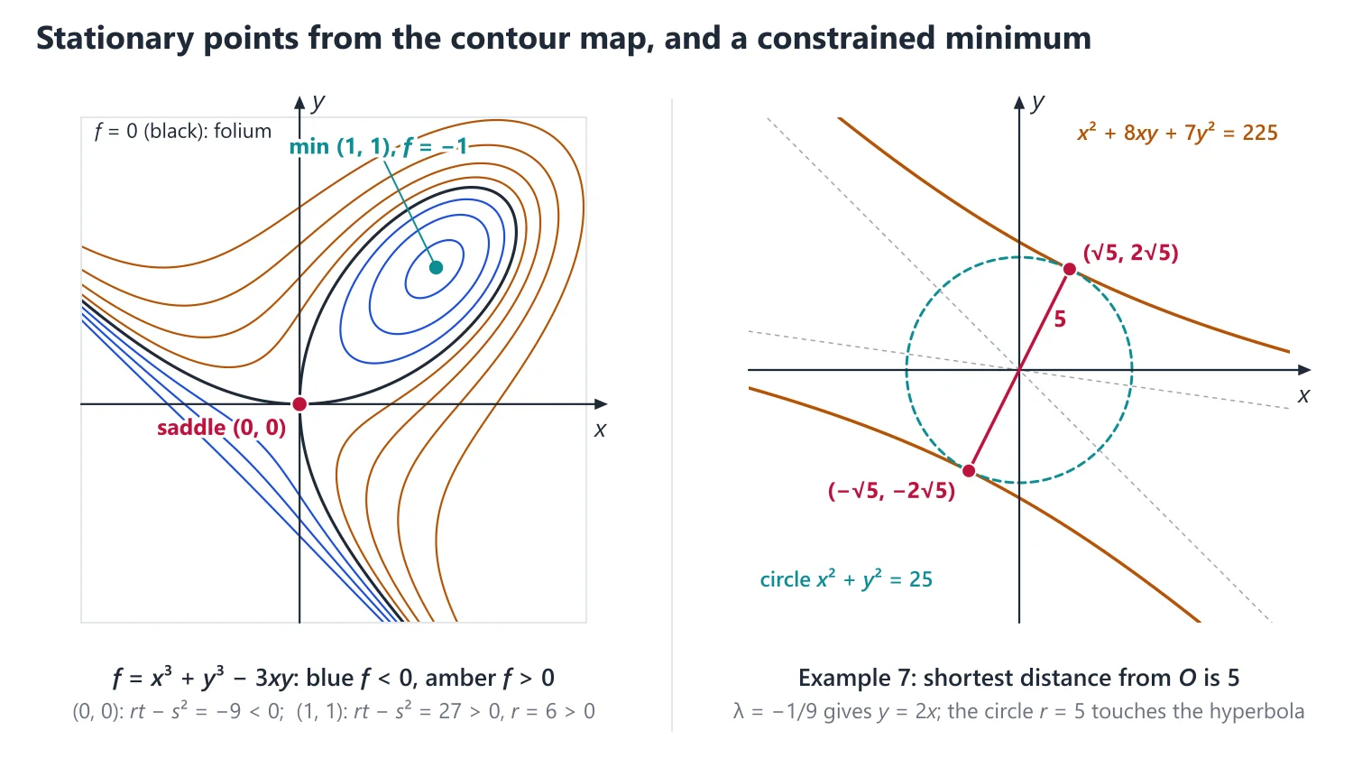
1. Understanding Limits in Two Variables
Why we need it: in one variable x can approach a only from the left or the right. In the plane (x, y) can approach (a, b) along infinitely many lines and curves, so a limit is a much stronger requirement, and many piecewise functions in UPSC questions fail it.
In words: f(x, y) → l as (x, y) → (a, b) if for every ε > 0 there is δ > 0 such that every point at distance less than δ from (a, b) (other than (a, b) itself) has |f(x, y) − l| < ε. The distance is √((x − a)2 + (y − b)2), and the direction of approach is not restricted.
Two practical consequences: to prove a limit, bound |f − l| by something depending only on the distance r; to disprove it, find two paths giving different limits.
First example, slowly: find lim(x, y)→(0, 0) (x3 + y3)/(x2 + y2).
Step 1 (guess): along y = 0 the function is x3/x2 = x → 0, so the only candidate is l = 0.
Step 2 (polar form): put x = r cos θ, y = r sin θ. Then f = r3(cos3θ + sin3θ)/r2 = r(cos3θ + sin3θ).
Step 3 (bound independent of θ): |cos3θ + sin3θ| ≤ 2, so |f − 0| ≤ 2r.
Step 4 (choose δ): given ε, δ = ε/2 works: r < δ ⇒ |f| < ε, whatever the direction. So the limit is 0.
Non-example: f = (x2 − y2)/(x2 + y2) in polar form is cos 2θ, which does not shrink with r. Along the x-axis the value is 1 and along the y-axis it is −1, so there is no limit at (0, 0).
Building up: (1) A bound |f − l| ≤ g(r) with g(r) → 0 proves the limit (the polar test). (2) A limit along every line is necessary but not sufficient: x2y/(x4 + y2) tends to 0 on all lines but is 1/2 on y = x2 (Example 5). (3) Continuity at (a, b) means the limit exists and equals f(a, b).
Where it is used: the first part of every 'discuss continuity, partial derivatives and differentiability at (0, 0)' question; the same polar bound later tests differentiability.
2. Understanding Partial Derivatives and Differentiability
Why we need it: in one variable 'has a derivative' already means 'has a tangent line' and implies continuity. In two variables the partial derivatives see only the two axis directions, so we need a stronger notion, differentiability, that captures a genuine tangent plane.
In words: fx(a, b) is the ordinary derivative of x ↦ f(x, b) at a, computed as a limit of a difference quotient. f is differentiable at (a, b) if the error E(h, k) = f(a + h, b + k) − f(a, b) − hfx − kfy is small compared with the distance ρ = √(h2 + k2), i.e. E/ρ → 0.
Logical chain: continuous partials near the point ⇒ differentiable ⇒ continuous and partials exist. None of the arrows can be reversed.
First example, slowly: f(x, y) = x2y2/(x2 + y2), f(0, 0) = 0. Is f differentiable at (0, 0)?
Step 1 (partials from the definition): f(h, 0) = 0, so fx(0, 0) = lim (f(h, 0) − f(0, 0))/h = 0; similarly fy(0, 0) = 0.
Step 2 (the error): E(h, k) = f(h, k) − 0 − 0 − 0 = h2k2/(h2 + k2).
Step 3 (compare with ρ): in polar form h = ρ cos θ, k = ρ sin θ, E = ρ2cos2θ sin2θ, so |E/ρ| = ρ cos2θ sin2θ ≤ ρ → 0.
Step 4 (conclude): f is differentiable at (0, 0) with df = 0·dx + 0·dy; its tangent plane there is z = 0.
Non-example: f = xy/√(x2 + y2), f(0, 0) = 0, is continuous with fx(0, 0) = fy(0, 0) = 0, but E/ρ = hk/(h2 + k2) = 1/2 along h = k. The error is not small compared with ρ, so f is not differentiable: the graph has a crease, not a tangent plane.
Building up: (1) Differentiable ⇒ continuous, since E → 0 and the linear part → 0. (2) Continuity of one partial near the point gives differentiability by the mean value theorem ('Why the sufficient condition works', above). (3) Mixed partials: fxy = fyx when one of them is continuous (Schwarz); at a special point compute each from the definition.
Where it is used: continuity–partials–differentiability questions at (0, 0); approximation by differentials; the chain rule and implicit differentiation, which need differentiability.
3. Understanding Stationary Points and the Second Derivative Test
Why we need it: to find the highest or lowest value of f(x, y) near a point, we first locate the candidates (where the tangent plane is horizontal) and then need a quick way to tell a peak from a pit from a pass.
In words: a stationary point solves fx = 0 and fy = 0. There, with r = fxx, s = fxy, t = fyy, the quadratic Q(h, k) = rh2 + 2shk + tk2 describes f near the point: f(a + h, b + k) − f(a, b) ≈ Q/2.
rt − s2 > 0 means Q keeps one sign (that of r): minimum if r > 0, maximum if r < 0. rt − s2 < 0 means Q takes both signs: saddle. rt − s2 = 0 means Q is degenerate and higher terms decide.
First example, slowly: classify the stationary points of f(x, y) = x2 − xy + y2 − 2x + y.
Step 1 (stationary equations): fx = 2x − y − 2 = 0 and fy = −x + 2y + 1 = 0.
Step 2 (solve): from the first, y = 2x − 2; substituting, −x + 4x − 4 + 1 = 0, so x = 1 and y = 0. The only stationary point is (1, 0).
Step 3 (second derivatives): r = 2, s = −1, t = 2, so rt − s2 = 4 − 1 = 3 > 0 and r > 0.
Step 4 (conclude): (1, 0) is a minimum, with f(1, 0) = 1 − 0 + 0 − 2 + 0 = −1. Because f is a quadratic with positive definite part, this is in fact the absolute minimum.
Non-example: f = x2 + y3 at (0, 0) has r = 2, s = 0, t = 0, so rt − s2 = 0 and the test is silent. Along the y-axis f = y3 takes both signs, so the origin is not an extremum, although the x-direction alone suggests a minimum.
Building up: (1) At an interior extremum each one-variable slice has zero derivative, so fx = fy = 0. (2) Taylor's theorem to second order gives f − f(a, b) = Q/2 + o(h2 + k2). (3) Completing the square, rQ = (rh + sk)2 + (rt − s2)k2, which shows the sign rules (Derivation 6).
Where it is used: 'find the extreme values of ...' questions; in three variables the same idea uses the leading minors of the Hessian; in Linear Algebra it is the definiteness of a quadratic form.
4. Understanding Lagrange's Multipliers
Why we need it: many problems ask for the extreme value of f subject to a condition, such as the largest box inside an ellipsoid. Solving the condition for one variable is often impossible or messy; Lagrange's method treats all variables symmetrically.
In words: at a constrained extremum of f on the surface φ = 0 (with ∇φ ≠ 0), the gradients are parallel: ∇f = −λ∇φ for some number λ, the multiplier. Equivalently, F = f + λφ has Fx = Fy = Fz = 0, and these equations with φ = 0 give the candidate points.
The method only produces candidates. Whether each is a maximum or a minimum must be argued separately, usually by compactness (a continuous f on a closed bounded constraint set attains both) or by the geometry.
First example, slowly: find the maximum and minimum of f = xy on the circle x2 + y2 = 2.
Step 1 (set up): F = xy + λ(x2 + y2 − 2). Fx = y + 2λx = 0 and Fy = x + 2λy = 0.
Step 2 (solve without dividing by zero): from the first y = −2λx; substituting, x(1 − 4λ2) = 0. If x = 0 then y = 0, which is not on the circle; so λ = ±1/2.
Step 3 (the points): λ = −1/2 gives y = x and 2x2 = 2, so (1, 1), (−1, −1) with f = 1; λ = 1/2 gives y = −x, so (1, −1), (−1, 1) with f = −1.
Step 4 (decide): the circle is closed and bounded and f is continuous, so both extremes exist and must be among these values: maximum 1, minimum −1. Check: xy ≤ (x2 + y2)/2 = 1.
Non-example: minimise x on the cusp curve y2 = x3. The minimum is at (0, 0), but there ∇f = (1, 0) and ∇φ = (−3x2, 2y) = (0, 0), so ∇f = −λ∇φ has no solution. The method misses points where ∇φ = 0; such points must be checked separately.
Building up: (1) Near a point with φy ≠ 0 the constraint defines y = y(x) (implicit function theorem). (2) f(x, y(x)) has an ordinary extremum, so fx + fyy′ = 0 with y′ = −φx/φy. (3) Setting λ = −fy/φy turns this into Fx = Fy = 0 (Derivation 7).
Where it is used: box-in-ellipsoid, distance from a point to a surface, and stationary values of x2 + y2 + z2 on central sections (20-mark UPSC questions); duality in Linear Programming is the same idea with inequality constraints.
5. Limits, Continuity and Partial Derivatives
Limit: f(x, y) → l as (x, y) → (a, b) if for every ε > 0 there is δ > 0 with |f(x, y) − l| < ε whenever 0 < √((x − a)2 + (y − b)2) < δ.
Idea: in the plane a point can be approached from infinitely many directions and along curved paths, and the limit must be the same along all of them. Agreement along every straight line is not enough: x2y/(x4 + y2) tends to 0 along every line through the origin but equals 1/2 along y = x2 (Example 5).
Polar test: put x = a + r cos θ, y = b + r sin θ. If |f − l| ≤ g(r) with g(r) → 0 independently of θ, the limit is l; for example |x2y/(x2 + y2)| = r|cos2θ sin θ| ≤ r → 0.
Path test: if the limit along two paths differs, the limit does not exist. For xy/(x2 + y2) along y = mx the value is m/(1 + m2), which depends on m, so there is no limit at (0, 0).
Repeated limits: limx→a limy→b f and limy→b limx→a f may exist and differ, or exist without the double limit existing.
Partial derivative: fx(a, b) = limh→0 (f(a + h, b) − f(a, b))/h, and similarly fy.
Idea: fx is the slope of the slice y = b of the graph. Partial derivatives look only along the two axes, so they say nothing about other directions, which is why a function can have both partials at a point and still be discontinuous there (Example 1).
6. Differentiability and Mixed Partials
Differentiability: f is differentiable at (a, b) if f(a + h, b + k) − f(a, b) = hfx(a, b) + kfy(a, b) + ε√(h2 + k2), with ε → 0 as (h, k) → (0, 0).
Idea: differentiable means the graph has a genuine tangent plane z = f(a, b) + hfx + kfy that approximates f in every direction, with an error small compared with the distance √(h2 + k2). Test: compute fx, fy at the point and check that (f(a + h, b + k) − f(a, b) − hfx − kfy)/√(h2 + k2) → 0, often in polar form.
Implications: differentiable ⇒ continuous and partial derivatives exist; the converse fails. A sufficient condition: fx, fy exist near (a, b) and one of them is continuous at (a, b).
Why the sufficient condition works: suppose fy exists at (a, b) and fx is continuous there. Write f(a + h, b + k) − f(a, b) = [f(a + h, b + k) − f(a, b + k)] + [f(a, b + k) − f(a, b)]. The first bracket is hfx(a + θh, b + k) by the mean value theorem, = h(fx(a, b) + ε1) with ε1 → 0 by continuity; the second is k(fy(a, b) + ε2) by the definition of fy. So the error is hε1 + kε2 = o(√(h2 + k2)).
Example 1: f(x, y) = xy/(x2 + y2), f(0, 0) = 0, has fx(0, 0) = fy(0, 0) = 0 (since f = 0 on both axes) but is not continuous at (0, 0), hence not differentiable.
Schwarz's theorem: if fx, fy, fxy exist in a neighbourhood of (a, b) and fxy is continuous at (a, b), then fyx(a, b) exists and equals fxy(a, b).
Idea: fxy and fyx are two different limits of the same double difference quotient (f(a + h, b + k) − f(a + h, b) − f(a, b + k) + f(a, b))/(hk), taken in opposite orders. Continuity of a mixed partial is what lets the order of the two limits be exchanged; without it they can differ, as in the counter-example below.
Young's theorem: if fx and fy are differentiable at (a, b), then fxy(a, b) = fyx(a, b).
Counter-example: for f = xy(x2 − y2)/(x2 + y2), f(0, 0) = 0, we get fx(0, y) = −y and fy(x, 0) = x, so fxy(0, 0) = −1 and fyx(0, 0) = 1 (here fxy = ∂/∂y(∂f/∂x)).
Euler's theorem: if f is homogeneous of degree n, then xfx + yfy = nf and x2fxx + 2xyfxy + y2fyy = n(n − 1)f.
Euler for a function of a homogeneous function: if z = f(u) is homogeneous of degree n in x, y, then xux + yuy = g(u) with g(u) = nf(u)/f′(u), and x2uxx + 2xyuxy + y2uyy = g(u)(g′(u) − 1).
Differentials and approximation: if f is differentiable at (a, b), then f(a + h, b + k) ≈ f(a, b) + hfx(a, b) + kfy(a, b) for small h, k, the error being o(√(h2 + k2)).
Local formulae: if f agrees with a polynomial (or any C1 function) on a whole neighbourhood of a point, including the point itself, then f is continuous and differentiable there; always check that a piecewise formula holds on a full neighbourhood.
Chain rule and implicit functions: if z = f(x, y), x = x(t), y = y(t), then dz/dt = fxdx/dt + fydy/dt; if f(x, y) = 0 with fy ≠ 0, then dy/dx = −fx/fy.
Why dy/dx = −fx/fy: along the curve f(x, y(x)) = 0, the chain rule gives fx + fy·dy/dx = 0. The chain rule needs f differentiable, not merely with partial derivatives, and fy ≠ 0 is the hypothesis of the implicit function theorem that guarantees y(x) exists.
Taylor's theorem: f(a + h, b + k) = f(a, b) + (h∂/∂x + k∂/∂y)f + (1/2!)(h∂/∂x + k∂/∂y)2f + ... + Rn, the derivatives being evaluated at (a, b).
7. Maxima and Minima
Necessary condition: if f has a local extremum at an interior point (a, b) where fx, fy exist, then fx = fy = 0 there (a stationary point).
Why it works: the one-variable function x ↦ f(x, b) has a local extremum at a, so its derivative fx(a, b) is 0; similarly fy(a, b) = 0. The condition is not sufficient: f = xy has fx = fy = 0 at the origin, which is a saddle point.
Second derivative test: let f have continuous second partial derivatives near a stationary point, and put r = fxx, s = fxy, t = fyy there: rt − s2 > 0 and r < 0 gives a maximum; rt − s2 > 0 and r > 0 gives a minimum; rt − s2 < 0 gives a saddle point; rt − s2 = 0 needs further investigation.
Why rt − s2 = 0 decides nothing: x4 + y4 (minimum), −x4 − y4 (maximum) and x4 − y4 (saddle) all have r = s = t = 0 at the origin; the higher-order terms decide.
Three variables: let D1 = fxx, D2, D3 be the leading principal minors of the Hessian [[fxx, fxy, fxz], [fyx, fyy, fyz], [fzx, fzy, fzz]]. All positive gives a minimum; D1 < 0, D2 > 0, D3 < 0 gives a maximum.
Absolute extrema on a closed bounded region D: a continuous f attains a maximum and a minimum on D. (1) Find the stationary points inside D. (2) Find the extreme values of f on the boundary, by parametrising it or by Lagrange's method. (3) Compare all these values; the largest is the absolute maximum and the smallest the absolute minimum.
Example 2: Find the extreme values of f(x, y) = x3 + y3 − 3xy.
fx = 3x2 − 3y = 0 and fy = 3y2 − 3x = 0 give y = x2, x = y2, so x4 = x and the points are (0, 0), (1, 1). Here r = 6x, s = −3, t = 6y. At (0, 0), rt − s2 = −9 < 0: saddle point. At (1, 1), rt − s2 = 27 > 0 and r = 6 > 0: minimum, with value −1.
8. Lagrange's Method of Multipliers
Method: to find extrema of f(x, y, z) subject to φ(x, y, z) = 0:
1. Form F = f + λφ.
2. Solve Fx = 0, Fy = 0, Fz = 0 together with φ = 0 for x, y, z and λ.
3. Decide the nature of each point from d2F (with dφ = 0), the bordered Hessian, or the geometry of the problem.
For two constraints φ = 0 and ψ = 0, use F = f + λφ + μψ.
Standard trick for quadratic problems: when f and the constraints are quadratic or linear forms, multiply Fx = 0, Fy = 0, Fz = 0 by x, y, z and add. Euler's theorem then expresses λ through the stationary value u, and substituting x, y, z back into the linear constraint gives an equation for u directly.
Central sections: for the ellipsoid ax2 + by2 + cz2 = 1 cut by the plane lx + my + nz = 0, the stationary values r2 of x2 + y2 + z2 satisfy l2/(1 − ar2) + m2/(1 − br2) + n2/(1 − cr2) = 0; the two roots are the squares of the semi-axes of the elliptic section.
Example 3: Find the maximum of xyz subject to x + y + z = a, with x, y, z > 0.
F = xyz + λ(x + y + z − a). Fx = yz + λ = 0, Fy = xz + λ = 0, Fz = xy + λ = 0 give yz = xz = xy, so x = y = z = a/3. The maximum value is a3/27.
Example 4: Find the minimum of x2 + y2 + z2 subject to ax + by + cz = p.
2x + λa = 0 and similarly for y, z give (x, y, z) = −(λ/2)(a, b, c); substituting, −(λ/2)(a2 + b2 + c2) = p. The minimum is p2/(a2 + b2 + c2), the squared distance of the plane from the origin.
9. Derivation: Euler's Theorem on Homogeneous Functions
First order: f is homogeneous of degree n if f(tx, ty) = tnf(x, y) for t > 0. Differentiating with respect to t by the chain rule, xfx(tx, ty) + yfy(tx, ty) = ntn−1f(x, y); putting t = 1 gives xfx + yfy = nf.
Second order: fx and fy are homogeneous of degree n − 1, so xfxx + yfxy = (n − 1)fx and xfyx + yfyy = (n − 1)fy. Multiply by x and y, add, and use fxy = fyx: x2fxx + 2xyfxy + y2fyy = (n − 1)(xfx + yfy) = n(n − 1)f.
For u with f(u) homogeneous: apply the first result to z = f(u): f′(u)(xux + yuy) = nf(u), so xux + yuy = nf(u)/f′(u) = g(u). Check: for u = sin−1((x2 + y2)/(x + y)), sin u is homogeneous of degree 1 and g(u) = sin u/cos u = tan u.
10. Derivation: The Second Derivative Test
At a stationary point Taylor's theorem gives f(a + h, b + k) − f(a, b) = (1/2)Q(h, k) + o(h2 + k2), where Q(h, k) = rh2 + 2shk + tk2.
For r ≠ 0, completing the square gives Q = (1/r)[(rh + sk)2 + (rt − s2)k2]. If rt − s2 > 0, the bracket is positive for (h, k) ≠ (0, 0), so Q has the sign of r in every direction; Q is then bounded away from 0 on the unit circle and dominates the o-term, giving a minimum for r > 0 and a maximum for r < 0.
If rt − s2 < 0, Q takes both signs (for example along k = 0 and along rh + sk = 0 when r ≠ 0), so f rises in some directions and falls in others: a saddle point. In matrix language, the test asks whether the Hessian [[r, s], [s, t]] is positive definite, negative definite or indefinite.
11. Derivation: Why Lagrange's Method Works
Let f(x, y) have an extremum on the curve φ(x, y) = 0 at a point where φy ≠ 0. Near it the curve is y = y(x) with y′ = −φx/φy, and x ↦ f(x, y(x)) has an ordinary extremum, so fx + fyy′ = 0, i.e. fxφy − fyφx = 0.
So ∇f is parallel to ∇φ, and with λ = −fy/φy we get fx + λφx = 0 and fy + λφy = 0, which are Fx = Fy = 0 for F = f + λφ.
Picture: at a constrained maximum the level curve f = c just touches the constraint curve; touching curves have a common normal, which is the parallel-gradient condition. Points where ∇φ = 0 are not covered and must be checked separately.
12. Choosing the Method
If a limit at a point is asked → for existence use the polar bound; for non-existence use two paths (lines y = mx, then parabolas y = mx2 if the lines agree).
If differentiability at a point is asked → get fx, fy there from the definition, then test the error quotient; if fx or fy is continuous near the point, differentiability follows at once.
If fxy(0, 0) is asked for a piecewise f → find fx(0, y) for y ≠ 0 and fx(0, 0) from the definition, then fxy(0, 0) = limk→0 (fx(0, k) − fx(0, 0))/k.
If an expression like xux + yuy is asked and u is a function of a homogeneous expression → Euler's theorem applied to f(u).
If free extrema are asked → stationary points, then rt − s2 (or the Hessian minors in three variables).
If extrema under a constraint are asked → Lagrange's multipliers, or direct substitution if the constraint is easy to solve; for quadratic f with a linear or quadratic constraint use the multiply-by-x, y, z trick.
If absolute extrema on a closed bounded region are asked → interior stationary points, boundary extrema, then compare the values.
13. Common Mistakes
Proving a limit exists from straight lines alone: agreement along all lines y = mx does not prove the limit; use a bound independent of the path.
'Partial derivatives exist, so f is differentiable (or continuous)': false, as xy/(x2 + y2) shows.
Differentiating the formula for (x, y) ≠ (0, 0) and substituting (0, 0): derivatives at the special point must come from the definition (difference quotients).
Concluding from rt − s2 = 0: the test is inconclusive; examine f near the point (along lines, or by sign arguments).
Losing solutions in Lagrange's equations: dividing by x, y or λ when it might be 0 discards stationary points; split into cases instead.
Applying Euler's theorem to a non-homogeneous u: for u = sin−1(...) or tan−1(...), apply it to sin u or tan u, which is the homogeneous function.
14. Connections
Link: the second derivative test is the definiteness of the Hessian, a real symmetric matrix whose eigenvalues are real (Linear Algebra); the same classification of quadratic forms reduces conics and conicoids to canonical form (Analytic Geometry).
Link: the gradient ∇f of the Vector Analysis chapter is normal to the level surfaces, which is the geometry behind ∇f = −λ∇φ; and in Linear Programming the dual variables play the role of multipliers attached to the constraints.
15. Worked Examples
Example 5: Let f(x, y) = x2y/(x4 + y2) for (x, y) ≠ (0, 0), f(0, 0) = 0. Show that f → 0 along every straight line through the origin, yet f is not continuous at (0, 0).
On y = mx: f = mx3/(x4 + m2x2) = mx/(x2 + m2) → 0 as x → 0 (for m = 0 it is identically 0); on the y-axis f = 0.
On the parabola y = x2: f = x4/(2x4) = 1/2 for every x ≠ 0.
So the limit along y = x2 is 1/2 ≠ 0 = f(0, 0); the double limit does not exist and f is discontinuous at the origin. Straight-line paths alone never prove that a limit exists.
Example 6: If u = sin−1((x2 + y2)/(x + y)), show that xux + yuy = tan u.
u itself is not homogeneous, but z = sin u = (x2 + y2)/(x + y) is homogeneous of degree 1.
By Euler's theorem, xzx + yzy = z, i.e. x cos u·ux + y cos u·uy = sin u.
Dividing by cos u (≠ 0) gives xux + yuy = tan u.
Example 7: Find the shortest distance from the origin to the curve x2 + 8xy + 7y2 = 225.
Extremise x2 + y2 with F = x2 + y2 + λ(x2 + 8xy + 7y2 − 225). Fx = 0 and Fy = 0 give x + λ(x + 4y) = 0 and y + λ(4x + 7y) = 0.
Multiplying by x and y and adding: x2 + y2 + λ(x2 + 8xy + 7y2) = 0, so r2 = x2 + y2 = −225λ.
A non-zero solution needs (1 + λ)(1 + 7λ) − 16λ2 = 0, i.e. 9λ2 − 8λ − 1 = 0, so λ = 1 or λ = −1/9.
r2 > 0 forces λ = −1/9, giving r2 = 25. The shortest distance is 5 (the curve is a hyperbola, so there is no maximum).
16. Solved Past UPSC Questions
Example 8 (UPSC 2014, 15 marks): Obtain ∂2f(0, 0)/∂x∂y and ∂2f(0, 0)/∂y∂x for the function
f(x, y) = xy(3x2 − 2y2)/(x2 + y2), (x, y) ≠ (0, 0)
f(x, y) = 0, (x, y) = (0, 0).
Also, discuss the continuity of ∂2f/∂x∂y and ∂2f/∂y∂x at (0, 0).
f = 0 on both axes, so fx(0, 0) = fy(0, 0) = 0. For y ≠ 0, fx(0, y) = limh→0 f(h, y)/h = lim y(3h2 − 2y2)/(h2 + y2) = −2y, which also holds at y = 0.
For x ≠ 0, fy(x, 0) = limk→0 f(x, k)/k = lim x(3x2 − 2k2)/(x2 + k2) = 3x, also true at x = 0.
Hence ∂2f/∂y∂x (0, 0) = ∂/∂y(fx) at (0, 0) = limk→0 (fx(0, k) − fx(0, 0))/k = −2, and ∂2f/∂x∂y (0, 0) = ∂/∂x(fy) at (0, 0) = limh→0 (fy(h, 0) − fy(0, 0))/h = 3.
Away from the origin f is a rational function with non-zero denominator, so both mixed partials exist near (0, 0). If either were continuous at (0, 0), Schwarz's theorem would make the two equal there; since −2 ≠ 3, neither is continuous at (0, 0).
(Convention: ∂2f/∂x∂y means ∂/∂x(∂f/∂y); with the opposite convention the two values are interchanged.)
Answer: ∂2f/∂x∂y (0, 0) = 3 and ∂2f/∂y∂x (0, 0) = −2; both mixed partials are discontinuous at (0, 0).
Example 9 (UPSC 2015, 15 marks): Find the absolute maximum and minimum values of the function f(x, y) = x2 + 3y2 − y over the region x2 + 2y2 ≤ 1.
D = {x2 + 2y2 ≤ 1} is closed and bounded and f is continuous, so absolute extrema exist.
Interior: fx = 2x = 0 and fy = 6y − 1 = 0 give (0, 1/6), which lies inside D, with f(0, 1/6) = 3/36 − 1/6 = −1/12.
Boundary: x2 = 1 − 2y2 with −1/√2 ≤ y ≤ 1/√2, so f = 1 − 2y2 + 3y2 − y = y2 − y + 1 = φ(y).
φ′(y) = 2y − 1 = 0 at y = 1/2 (x = ±1/√2), where φ = 3/4. At the end points: y = 1/√2 (x = 0) gives 3/2 − 1/√2 ≈ 0.793, and y = −1/√2 (x = 0) gives 3/2 + 1/√2 ≈ 2.207.
Comparing −1/12, 3/4, 3/2 − 1/√2 and 3/2 + 1/√2 (a grid search over D confirms the result):
Answer: absolute maximum 3/2 + 1/√2 at (0, −1/√2); absolute minimum −1/12 at (0, 1/6).
Example 10 (UPSC 2019, 10 marks): Show that the function
f(x, y) = (x2 − y2)/(x − y), (x, y) ≠ (1, −1), (1, 1)
= 0, (x, y) = (1, 1), (1, −1)
is continuous and differentiable at (1, −1).
On N = {|x − 1| < 1/2, |y + 1| < 1/2} we have x > 1/2 > −1/2 > y, so x ≠ y, and (x2 − y2)/(x − y) = x + y at every point of N other than (1, −1).
At (1, −1) itself f = 0 = 1 + (−1). Hence f(x, y) = x + y on the whole neighbourhood N.
A polynomial is continuous, so f is continuous at (1, −1).
fx(1, −1) = fy(1, −1) = 1, and f(1 + h, −1 + k) − f(1, −1) = h + k exactly for small h, k, so the remainder is 0 and f is differentiable at (1, −1) with df = dx + dy.
(At (1, 1) it is different: x + y → 2 ≠ 0 = f(1, 1), so f is discontinuous there.)
Answer: f coincides with x + y near (1, −1), so it is continuous and differentiable there, with fx = fy = 1.
Example 11 (UPSC 2019, 15 marks): Using differentials, find an approximate value of f(4.1, 4.9) where
f(x, y) = (x3 + x2y)1/2.
Take (a, b) = (4, 5), h = 0.1, k = −0.1. f(4, 5) = √(64 + 80) = √144 = 12.
fx = (3x2 + 2xy)/(2√(x3 + x2y)) = (48 + 40)/24 = 11/3 at (4, 5), and fy = x2/(2√(x3 + x2y)) = 16/24 = 2/3.
df = fxh + fyk = (11/3)(0.1) + (2/3)(−0.1) = 0.3.
So f(4.1, 4.9) ≈ 12 + 0.3 = 12.3. (Here the approximation happens to be exact: 4.13 + 4.12·4.9 = 4.12·9 = 151.29 = 12.32.)
Answer: f(4.1, 4.9) ≈ 12.3.
Example 12 (UPSC 2020, 20 marks): If u = tan−1((x3 + y3)/(x − y)), x ≠ y, then show that x2 ∂2u/∂x2 + 2xy ∂2u/∂x∂y + y2 ∂2u/∂y2 = (1 − 4 sin2u) sin 2u
Let z = tan u = (x3 + y3)/(x − y), which is homogeneous of degree 3 − 1 = 2.
By Euler, xzx + yzy = 2z, i.e. sec2u(xux + yuy) = 2 tan u, so xux + yuy = 2 sin u cos u = sin 2u = g(u).
Differentiate xux + yuy = g(u) with respect to x and to y: ux + xuxx + yuxy = g′(u)ux and xuxy + uy + yuyy = g′(u)uy.
Multiply by x and y and add: x2uxx + 2xyuxy + y2uyy = (g′(u) − 1)(xux + yuy) = g(u)(g′(u) − 1).
With g(u) = sin 2u, g′(u) = 2 cos 2u, so the right side is sin 2u(2 cos 2u − 1) = sin 2u(2(1 − 2 sin2u) − 1) = (1 − 4 sin2u) sin 2u.
Answer: x2uxx + 2xyuxy + y2uyy = (1 − 4 sin2u) sin 2u, as required.
Example 13 (UPSC 2021, 20 marks): Find the stationary values of x2 + y2 + z2 subject to the conditions ax2 + by2 + cz2 = 1 and lx + my + nz = 0. Interpret the result geometrically.
F = x2 + y2 + z2 + λ(ax2 + by2 + cz2 − 1) + μ(lx + my + nz). Fx = 0 gives 2x + 2λax + μl = 0, and similarly 2y + 2λby + μm = 0, 2z + 2λcz + μn = 0.
Multiply by x, y, z and add. With u = x2 + y2 + z2 and the two constraints, 2u + 2λ = 0, so λ = −u.
Then 2x(1 − au) = −μl, so x = −μl/(2(1 − au)); similarly y = −μm/(2(1 − bu)) and z = −μn/(2(1 − cu)) (in the general case 1 − au, 1 − bu, 1 − cu ≠ 0; then μ ≠ 0, otherwise x = y = z = 0).
Substituting in lx + my + nz = 0 gives l2/(1 − au) + m2/(1 − bu) + n2/(1 − cu) = 0.
Clearing denominators, l2(1 − bu)(1 − cu) + m2(1 − cu)(1 − au) + n2(1 − au)(1 − bu) = 0, a quadratic in u whose two roots are the stationary (maximum and minimum) values. (Check: a = 1, b = 2, c = 3, l = m = n = 1 gives u ≈ 0.388 and 0.703, matching a direct numerical search.)
Geometrically, the plane through the centre cuts the ellipsoid in an ellipse, and u is the squared distance of a point of this ellipse from the centre; so the roots are the squares of the semi-axes of this central section.
Answer: the stationary values u of x2 + y2 + z2 are the roots of l2/(1 − au) + m2/(1 − bu) + n2/(1 − cu) = 0; they are the squared semi-axes of the section of the ellipsoid by the plane.
Example 14 (UPSC 2022, 20 marks): Find the maximum and minimum values of x2/a4 + y2/b4 + z2/c4, when lx + my + nz = 0 and x2/a2 + y2/b2 + z2/c2 = 1. Interpret the result geometrically.
F = x2/a4 + y2/b4 + z2/c4 + λ(x2/a2 + y2/b2 + z2/c2 − 1) + μ(lx + my + nz). Fx = 0 gives 2x/a4 + 2λx/a2 + μl = 0, and similarly for y, z.
Multiply by x, y, z and add; with u = x2/a4 + y2/b4 + z2/c4 this gives 2u + 2λ = 0, so λ = −u.
Then 2x(1 − a2u)/a4 = −μl, so x = −μla4/(2(1 − a2u)); similarly for y and z.
Substituting in lx + my + nz = 0 (μ ≠ 0 as before): l2a4/(1 − a2u) + m2b4/(1 − b2u) + n2c4/(1 − c2u) = 0, a quadratic in u whose roots are the maximum and minimum values. (Check: a = 1, b = 2, c = 3, l = m = n = 1 gives u ≈ 0.207 and 0.940 both from this equation and from a direct search.)
Geometric meaning: the tangent plane to the ellipsoid at (x, y, z) is Xx/a2 + Yy/b2 + Zz/c2 = 1, whose distance p from the centre satisfies 1/p2 = x2/a4 + y2/b4 + z2/c4.
Answer: the extreme values are the roots u of ∑ l2a4/(1 − a2u) = 0; they are the extreme values of 1/p2, where p is the perpendicular from the centre to the tangent planes at points of the central section by lx + my + nz = 0.
Example 15 (UPSC 2023, 15 marks): Using the method of Lagrange's multipliers, find the minimum and maximum distances of the point P(2, 6, 3) from the sphere x2 + y2 + z2 = 4.
Extremise D = (x − 2)2 + (y − 6)2 + (z − 3)2 subject to x2 + y2 + z2 = 4, with F = D + λ(x2 + y2 + z2 − 4).
Fx = 2(x − 2) + 2λx = 0 gives x = 2/(1 + λ); similarly y = 6/(1 + λ) and z = 3/(1 + λ).
Substituting in the constraint: (4 + 36 + 9)/(1 + λ)2 = 4, so 1 + λ = ±7/2.
1 + λ = 7/2 gives (4/7, 12/7, 6/7) and D = (100 + 900 + 225)/49 = 25; 1 + λ = −7/2 gives (−4/7, −12/7, −6/7) and D = (324 + 2916 + 729)/49 = 81.
Check: |OP| = √49 = 7, and the nearest and farthest points of the sphere lie on line OP at distances 7 − 2 and 7 + 2.
Answer: minimum distance 5 (at (4/7, 12/7, 6/7)) and maximum distance 9 (at (−4/7, −12/7, −6/7)).
Example 16 (UPSC 2025, 20 marks): Show that the volume of the greatest rectangular parallelopiped that can be inscribed in the ellipsoid x2/a2 + y2/b2 + z2/c2 = 1 is 8abc/(3√3).
By symmetry the vertices are (±x, ±y, ±z) with x, y, z > 0 on the ellipsoid, and the volume is V = 8xyz.
F = xyz + λ(x2/a2 + y2/b2 + z2/c2 − 1). Fx = yz + 2λx/a2 = 0, Fy = xz + 2λy/b2 = 0, Fz = xy + 2λz/c2 = 0.
Multiplying by x, y, z: xyz = −2λx2/a2 = −2λy2/b2 = −2λz2/c2. As xyz ≠ 0, x2/a2 = y2/b2 = z2/c2, and their sum is 1, so each equals 1/3.
So x = a/√3, y = b/√3, z = c/√3 and V = 8abc/(3√3).
This is the maximum: V is continuous on the compact part of the ellipsoid with x, y, z ≥ 0, vanishes on its edges (where a coordinate is 0), and has only this stationary point inside.
Answer: the greatest volume is 8abc/(3√3).
17. Practice Exercises
Exercise 1 (basic): Find fx and fy for f(x, y) = x2y + exy.
Answer: fx = 2xy + yexy, fy = x2 + xexy.
Exercise 2 (basic): Show that lim(x, y)→(0, 0) x2/(x2 + y2) does not exist.
Answer: along y = mx the value is 1/(1 + m2), which depends on m.
Exercise 3 (basic): Verify Euler's theorem for f = x3 + x2y + y3.
Answer: xfx + yfy = x(3x2 + 2xy) + y(x2 + 3y2) = 3x3 + 3x2y + 3y3 = 3f (degree 3).
Exercise 4 (standard): Find lim(x, y)→(0, 0) x3/(x2 + y2).
Answer: 0, since in polar form |f| = r|cos3θ| ≤ r.
Exercise 5 (standard): Find and classify the stationary points of f = x2 + xy + y2 − 3x.
Answer: 2x + y = 3, x + 2y = 0 give (2, −1); r = 2, s = 1, t = 2, rt − s2 = 3 > 0, r > 0: minimum value f(2, −1) = −3.
Exercise 6 (standard): Is f(x, y) = √|xy| differentiable at (0, 0)?
Answer: no: fx(0, 0) = fy(0, 0) = 0, but E/ρ = √|hk|/√(h2 + k2) = 1/√2 along h = k (f is continuous there).
Exercise 7 (standard): Using Lagrange's method, find the extreme values of x + y on x2 + y2 = 1.
Answer: 1 + 2λx = 1 + 2λy = 0 gives x = y = ±1/√2: maximum √2, minimum −√2.
Exercise 8 (UPSC level): Find the extreme values of f(x, y) = x3 + 3xy2 − 15x2 − 15y2 + 72x.
Answer: stationary points (4, 0), (6, 0), (5, ±1); r = t = 6x − 30, s = 6y. Maximum 112 at (4, 0), minimum 108 at (6, 0); (5, ±1) are saddle points (rt − s2 = −36).
Exercise 9 (UPSC level): Find the minimum of x2 + y2 + z2 subject to xyz = a3, a > 0.
Answer: 2x + λyz = 0 etc.; multiplying by x, y, z gives x2 = y2 = z2 = a2, so the minimum is 3a2 (at (a, a, a) and the sign changes with xyz > 0); AM–GM confirms it.
Exercise 10 (UPSC level): For f(x, y) = x2 tan−1(y/x) − y2 tan−1(x/y) (xy ≠ 0), f = 0 on the axes, find fxy(0, 0) = ∂/∂y(∂f/∂x) and fyx(0, 0) = ∂/∂x(∂f/∂y) at (0, 0).
Answer: fx(0, y) = lim f(h, y)/h = −y and fy(x, 0) = x, so fxy(0, 0) = −1 and fyx(0, 0) = 1; the mixed partials are unequal (and hence not continuous at the origin).
| rt − s2 | r = fxx | Nature |
|---|---|---|
| > 0 | > 0 | Local minimum |
| > 0 | < 0 | Local maximum |
| < 0 | any | Saddle point (no extremum) |
| = 0 | any | Doubtful: examine f(a + h, b + k) − f(a, b) directly |
Mains points
- A standard question gives a function defined piecewise at (0, 0) and asks about continuity, existence of partial derivatives, differentiability and equality of fxy, fyx; compute partials at the origin from the definition, not by formula.
- For unconstrained extrema, list all stationary points, tabulate r, s, t and rt − s2 for each, and state the nature and the value; missing a stationary point is a common error.
- For Lagrange multiplier problems (volume of box in an ellipsoid, distance from a point to a surface), set up F clearly and justify why the point found is a maximum or minimum.
- When rt − s2 = 0, examine the sign of f(a + h, b + k) − f(a, b) along suitable paths instead of stopping.
- State Schwarz's or Young's theorem with hypotheses when asked to show fxy = fyx, and give the standard counter-example when asked whether they are always equal.
Did you know?
- Memory trick for the 2-variable test: 'rt − s2 positive means a peak or a pit; negative means a pass (saddle)'; r then tells peak (r < 0) from pit (r > 0).
Standard Proofs: Real Analysis
Eighteen classical theorems of real analysis that UPSC asks candidates to prove: completeness results (monotone convergence, Bolzano–Weierstrass, Cauchy criterion), series tests, the properties of continuous functions on [a, b], integrability and the fundamental theorem, and the basic uniform convergence theorems. Every proof is ε-based and uses only the completeness axiom and earlier results.
1. Archimedean Property
Statement: If x > 0 and y ∈ ℝ, then there is n ∈ ℕ with nx > y. In particular 1/n → 0.
Proof: Suppose not. Then nx ≤ y for every n ∈ ℕ, so S = {nx : n ∈ ℕ} is non-empty and bounded above by y.
By the completeness axiom s = sup S exists. Since x > 0, s − x < s, so s − x is not an upper bound of S.
Hence mx > s − x for some m ∈ ℕ, i.e. (m + 1)x > s. But (m + 1)x ∈ S, contradicting s = sup S.
For the last part, given ε > 0 apply the property with x = ε, y = 1 to get N with Nε > 1; then 0 < 1/n ≤ 1/N < ε for all n ≥ N.
Hence proved.
2. Monotone Convergence Theorem
Statement: An increasing sequence (an) of real numbers that is bounded above converges, and lim an = sup{an : n ∈ ℕ}. Similarly a decreasing sequence bounded below converges to its infimum.
Proof: The set {an} is non-empty and bounded above, so l = sup{an} exists by completeness.
Let ε > 0. Since l − ε is not an upper bound, aN > l − ε for some N.
For n ≥ N, monotonicity gives l − ε < aN ≤ an ≤ l < l + ε, so |an − l| < ε. Hence an → l.
If (an) is decreasing and bounded below, (−an) is increasing and bounded above, so −an → sup(−an) = −inf an, i.e. an → inf an.
Hence proved.
3. Bolzano–Weierstrass Theorem
Statement: Every bounded sequence of real numbers has a convergent subsequence.
Proof: Call an index m a peak if am ≥ an for every n > m. We show (an) has a monotone subsequence.
Case 1: there are infinitely many peaks m1 < m2 < .... Then am1 ≥ am2 ≥ ... is a decreasing subsequence.
Case 2: there are finitely many peaks. Choose n1 larger than all of them. Since n1 is not a peak, there is n2 > n1 with an2 > an1; n2 is not a peak either, so there is n3 > n2 with an3 > an2, and so on.
This gives a strictly increasing subsequence.
In both cases the monotone subsequence is bounded, because (an) is bounded, so it converges by the monotone convergence theorem.
Hence proved.
4. Cauchy's General Principle of Convergence
Statement: A sequence (an) of real numbers converges iff it is a Cauchy sequence.
Proof: (⇒) Let an → l and ε > 0. Choose N with |an − l| < ε/2 for n ≥ N. Then for m, n ≥ N, |am − an| ≤ |am − l| + |l − an| < ε.
(⇐) Let (an) be Cauchy. With ε = 1 there is N0 such that |an| ≤ |aN0| + 1 for n ≥ N0, so |an| ≤ max(|a1|, ..., |aN0|) + 1 for all n: the sequence is bounded.
By Bolzano–Weierstrass some subsequence ank → l.
Let ε > 0. Choose N with |am − an| < ε/2 for m, n ≥ N, and then k with nk ≥ N and |ank − l| < ε/2 (possible since nk → ∞ and ank → l).
For n ≥ N, |an − l| ≤ |an − ank| + |ank − l| < ε/2 + ε/2 = ε. Hence an → l.
Hence proved.
5. Cauchy's First Theorem on Limits
Statement: If an → l, then (a1 + a2 + ... + an)/n → l.
Proof: Put bn = an − l, so bn → 0; it suffices to show (b1 + ... + bn)/n → 0, since this equals (a1 + ... + an)/n − l.
A convergent sequence is bounded, so |bn| ≤ M for all n.
Let ε > 0 and choose N with |bn| < ε/2 for n > N. For n > N, |b1 + ... + bn|/n ≤ (|b1| + ... + |bN|)/n + ((n − N)/n)(ε/2) ≤ NM/n + ε/2.
Choose N1 ≥ N with NM/N1 < ε/2. Then for n > N1 the expression is less than ε/2 + ε/2 = ε.
Hence (b1 + ... + bn)/n → 0, and the arithmetic means of (an) tend to l.
Hence proved.
6. Absolute Convergence Implies Convergence
Statement: If ∑|an| converges, then ∑an converges, and |∑an| ≤ ∑|an|.
Proof: Applying Cauchy's principle to the partial sums gives the Cauchy criterion for series: ∑un converges iff for every ε > 0 there is N with |un+1 + ... + um| < ε for all m > n ≥ N.
Since ∑|an| converges, for ε > 0 there is N with |an+1| + ... + |am| < ε for all m > n ≥ N.
By the triangle inequality, |an+1 + ... + am| ≤ |an+1| + ... + |am| < ε for the same m, n.
So ∑an satisfies the Cauchy criterion and converges. Letting n → ∞ in |a1 + ... + an| ≤ |a1| + ... + |an| gives |∑an| ≤ ∑|an|.
Hence proved.
7. Leibniz's Test for Alternating Series
Statement: If (un) is a decreasing sequence of positive terms with un → 0, then ∑(−1)n+1un converges, and its sum S satisfies 0 ≤ S ≤ u1. Applying this to the tail un+1 − un+2 + ⋯ gives the error bound |S − Sn| ≤ un+1.
Proof: Let Sn be the partial sums. S2n+2 − S2n = u2n+1 − u2n+2 ≥ 0, so (S2n) is increasing; also S2n = (u1 − u2) + ... + (u2n−1 − u2n) ≥ 0.
S2n = u1 − (u2 − u3) − ... − (u2n−2 − u2n−1) − u2n ≤ u1, since every bracket is non-negative.
By the monotone convergence theorem S2n → S for some S with 0 ≤ S ≤ u1.
S2n+1 = S2n + u2n+1 → S + 0 = S.
Given ε > 0, choose N1, N2 with |S2n − S| < ε for n ≥ N1 and |S2n+1 − S| < ε for n ≥ N2; then |Sm − S| < ε for all m ≥ 2max(N1, N2) + 1. So Sn → S.
Hence proved.
8. D'Alembert's Ratio Test
Statement: Let an > 0 and an+1/an → l. If l < 1 then ∑an converges; if l > 1 then ∑an diverges.
Proof: Let l < 1 and fix r with l < r < 1. Taking ε = r − l, there is N with an+1/an < r for all n ≥ N.
Then aN+1 < raN, aN+2 < r2aN, and in general an ≤ aNrn−N = (aNr−N)rn for n ≥ N.
∑rn converges because 0 < r < 1, so ∑an converges by the comparison test (finitely many initial terms do not affect convergence).
Let l > 1. Taking ε = l − 1, there is N with an+1/an > 1 for n ≥ N, so an ≥ aN > 0 for all n ≥ N.
Then an does not tend to 0, so ∑an diverges. (For l = 1 no conclusion: ∑1/n diverges while ∑1/n2 converges, both with l = 1.)
Hence proved.
9. A Continuous Function on [a, b] is Bounded and Attains its Bounds
Statement: Let f be continuous on the closed bounded interval [a, b]. Then f is bounded, and there are points c, d ∈ [a, b] with f(c) = sup f and f(d) = inf f.
Proof: Suppose f is unbounded. Then for each n there is xn ∈ [a, b] with |f(xn)| > n.
(xn) is bounded, so by Bolzano–Weierstrass a subsequence xnk → c, and a ≤ xnk ≤ b gives c ∈ [a, b].
By continuity f(xnk) → f(c), so (f(xnk)) is bounded; but |f(xnk)| > nk → ∞. This contradiction shows f is bounded.
Let M = sup f, which exists by completeness. For each n there is yn ∈ [a, b] with M − 1/n < f(yn) ≤ M.
Again a subsequence ynk → c ∈ [a, b], and f(ynk) → M by the sandwich theorem. Continuity gives f(c) = M.
Applying this to −f gives a point d with f(d) = inf f.
Hence proved.
10. Intermediate Value Theorem
Statement: Let f be continuous on [a, b] and let k lie strictly between f(a) and f(b). Then f(c) = k for some c ∈ (a, b).
Proof: Assume f(a) < k < f(b); otherwise apply the argument to −f and −k.
Let S = {x ∈ [a, b] : f(x) < k}. S contains a and is bounded above by b, so c = sup S exists and a ≤ c ≤ b.
Suppose f(c) < k. Then c ≠ b (as f(b) > k), and by continuity there is δ > 0 with f(x) < k for x ∈ [c, c + δ) ∩ [a, b]. These include points of S greater than c, contradicting c = sup S.
Suppose f(c) > k. Then c ≠ a (as f(a) < k), and by continuity there is δ with 0 < δ < c − a and f(x) > k on (c − δ, c]. Then no point of S lies in (c − δ, c], and no point of S exceeds c, so c − δ is an upper bound of S, contradicting c = sup S.
Hence f(c) = k, and c ≠ a, b because f(a) ≠ k ≠ f(b).
Hence proved.
11. Heine–Cantor Theorem (Uniform Continuity on [a, b])
Statement: A function f continuous on a closed bounded interval [a, b] is uniformly continuous on [a, b].
Proof: Suppose not. Then there is ε0 > 0 such that for every δ > 0 some pair x, y ∈ [a, b] has |x − y| < δ but |f(x) − f(y)| ≥ ε0.
Taking δ = 1/n gives xn, yn ∈ [a, b] with |xn − yn| < 1/n and |f(xn) − f(yn)| ≥ ε0.
By Bolzano–Weierstrass a subsequence xnk → c, with c ∈ [a, b] since the interval is closed. As |xnk − ynk| < 1/nk → 0, also ynk → c.
By continuity at c, f(xnk) − f(ynk) → f(c) − f(c) = 0, contradicting |f(xnk) − f(ynk)| ≥ ε0.
Hence f is uniformly continuous. Both closedness and boundedness are needed: 1/x on (0, 1] and x2 on ℝ are continuous but not uniformly continuous.
Hence proved.
12. Every Continuous Function on [a, b] is Riemann Integrable
Statement: If f is continuous on [a, b], then f ∈ R[a, b].
Proof: f is bounded (previous theorem), so the upper and lower sums are defined.
Let ε > 0. By the Heine–Cantor theorem there is δ > 0 such that |x − y| < δ ⇒ |f(x) − f(y)| < ε/(b − a).
Take any partition P with every Δxi < δ. On [xi−1, xi], f attains Mi and mi at two points less than δ apart, so Mi − mi < ε/(b − a).
Then U(P, f) − L(P, f) = ∑(Mi − mi)Δxi < (ε/(b − a))∑Δxi = ε.
By Riemann's criterion, f ∈ R[a, b].
Hence proved.
13. First Fundamental Theorem of Integral Calculus
Statement: Let f ∈ R[a, b] and F(x) = ∫ax f(t) dt for x ∈ [a, b]. Then F is continuous on [a, b], and if f is continuous at c ∈ [a, b], F is differentiable at c with F′(c) = f(c) (one-sided at an end point).
Proof: An integrable function is bounded, say |f| ≤ M. For x, y ∈ [a, b], |F(y) − F(x)| = |∫xy f(t) dt| ≤ M|y − x|, so F is (uniformly) continuous.
Let f be continuous at c. For h ≠ 0 with c + h ∈ [a, b], (F(c + h) − F(c))/h − f(c) = (1/h)∫cc+h (f(t) − f(c)) dt, because ∫cc+h f(c) dt = hf(c).
Given ε > 0, choose δ > 0 with |f(t) − f(c)| < ε whenever |t − c| < δ.
For 0 < |h| < δ, every t between c and c + h satisfies |t − c| < δ, so |(F(c + h) − F(c))/h − f(c)| ≤ (1/|h|)·ε|h| = ε.
Hence F′(c) = f(c).
Hence proved.
14. The Uniform Limit of Continuous Functions is Continuous
Statement: Let each fn be continuous at c ∈ E and let fn → f uniformly on E. Then f is continuous at c. Hence the sum of a uniformly convergent series of continuous functions is continuous.
Proof: Let ε > 0. By uniform convergence choose N with |fN(x) − f(x)| < ε/3 for all x ∈ E.
fN is continuous at c, so there is δ > 0 with |fN(x) − fN(c)| < ε/3 for x ∈ E, |x − c| < δ.
For such x, |f(x) − f(c)| ≤ |f(x) − fN(x)| + |fN(x) − fN(c)| + |fN(c) − f(c)| < ε/3 + ε/3 + ε/3 = ε.
So f is continuous at c. Applying this to the partial sums Sn = u1 + ... + un gives the statement for series.
Contrapositive used in practice: if continuous fn converge to a discontinuous limit, the convergence is not uniform (for example xn on [0, 1]).
Hence proved.
15. Weierstrass M-test
Statement: Let |un(x)| ≤ Mn for all x ∈ E and all n, where ∑Mn is a convergent series of constants. Then ∑un(x) converges uniformly and absolutely on E.
Proof: Let ε > 0. By the Cauchy criterion for ∑Mn, there is N with Mn+1 + ... + Mm < ε for all m > n ≥ N; note that N does not involve x.
For every x ∈ E and m > n ≥ N, |un+1(x) + ... + um(x)| ≤ |un+1(x)| + ... + |um(x)| ≤ Mn+1 + ... + Mm < ε.
So the partial sums Sn(x) satisfy |Sm(x) − Sn(x)| < ε for all x ∈ E and m > n ≥ N: by the Cauchy criterion for uniform convergence, ∑un converges uniformly on E.
The middle inequality shows that ∑|un(x)| also satisfies the Cauchy criterion, so the convergence is absolute as well.
Hence proved.
16. A Monotone Function on [a, b] is Riemann Integrable
Statement: Let f be monotone on [a, b]. Then f ∈ R[a, b].
Proof: Suppose f is increasing (for decreasing f apply the argument to −f). Then f(a) ≤ f(x) ≤ f(b), so f is bounded. If f(a) = f(b), f is constant and integrable, so let f(b) > f(a).
Given ε > 0, let P divide [a, b] into n equal parts of length h = (b − a)/n, with n so large that (f(b) − f(a))(b − a)/n < ε.
Since f is increasing, on [xi−1, xi] we have Mi = f(xi) and mi = f(xi−1).
So U(P, f) − L(P, f) = ∑i=1n (f(xi) − f(xi−1))h = h(f(b) − f(a)) < ε, the sum telescoping.
By Riemann's criterion, f ∈ R[a, b].
Hence proved.
17. A Contractive Sequence is Cauchy
Statement: Let (an) be a real sequence with |an+1 − an| ≤ α|an − an−1| for all n ≥ 2, where 0 < α < 1. Then (an) is a Cauchy sequence, and hence convergent.
Proof: Let d = |a2 − a1|. Applying the hypothesis repeatedly, |an+1 − an| ≤ α|an − an−1| ≤ ⋯ ≤ αn−1d for all n ≥ 1.
For m > n, by the triangle inequality, |am − an| ≤ |am − am−1| + ⋯ + |an+1 − an| ≤ d(αm−2 + ⋯ + αn−1).
The geometric sum is less than αn−1/(1 − α), so |am − an| < dαn−1/(1 − α).
Since 0 < α < 1, αn−1 → 0. Given ε > 0 choose N with dαN−1/(1 − α) < ε (any N works if d = 0); then |am − an| < ε for all m > n ≥ N.
So (an) is Cauchy, and by Cauchy's general principle it converges.
Hence proved.
18. Riemann's Rearrangement Theorem
Statement: Let ∑xn be a conditionally convergent series of real numbers and S any real number (for example S = 100). Then some rearrangement ∑xπ(n) converges to S.
Proof: Let p1, p2, ... be the non-negative terms and q1, q2, ... the absolute values of the negative terms, each in their original order; both lists are infinite.
∑pk and ∑qk both diverge: if both converged, ∑|xn| would converge, and if exactly one converged, ∑xn would diverge. Also pk → 0 and qk → 0, since xn → 0.
Build the rearrangement in blocks: take p1, p2, ... until the partial sum first exceeds S, then −q1, −q2, ... until it first falls below S, then positive terms again, and so on.
Each block is finite because the unused positive (and negative) terms still have an infinite sum. So the process never stops, and every term of the original series is used exactly once: the result is a rearrangement.
After a positive block ends, the partial sum T satisfies S < T ≤ S + p, where p is the last term used; during the next negative block the partial sums decrease from T to a value at least S − q, where q is the last term of that block. So every partial sum after the first block lies within max(p, q) of S for the most recent block-end terms p, q.
The block-end terms are pk, qk with k → ∞, and these tend to 0, so the partial sums of the rearranged series converge to S. Taking S = 100 gives a rearrangement with sum 100.
Hence proved.
Mains points
- Most frequently asked: Heine–Cantor (continuous on [a, b] ⇒ uniformly continuous), 'a continuous function on [a, b] is bounded and attains its bounds', the intermediate value theorem, Cauchy's general principle, and the M-test or continuity of a uniform limit.
- Write ε-δ and ε-N arguments in a fixed order: 'Let ε > 0', choose N or δ with a stated reason, take an arbitrary n ≥ N or |x − c| < δ, estimate, conclude. Omitting 'Let ε > 0' or the reason for the choice of δ is penalised.
- Name the completeness tool you are using (supremum axiom, monotone convergence, Bolzano–Weierstrass); each of these proofs fails over ℚ, and examiners look for where completeness enters.
- When a proof is by contradiction through sequences (boundedness, Heine–Cantor), say explicitly why the limit of the subsequence lies in [a, b]; this is the step that uses closedness.
- Under time pressure the ε/3 argument (uniform limit), the ε/2 argument (Cauchy ⇒ convergent) and the geometric comparison (ratio test) can each be written in four lines; practise them until they are automatic.
Did you know?
- Bolzano proved the intermediate value theorem in 1817 precisely because he felt the 'obvious' geometric argument was not a proof; his work was largely ignored until Weierstrass rediscovered the same ideas fifty years later.
Solved Problems: Real Analysis
Thirteen UPSC-style problems covering sequences and series, continuity and Riemann integration, and uniform convergence and functions of several variables, each with a complete step-by-step solution and a stated answer.
1. Sequences and Series
Problem 1 (10 marks): Show that the sequence an = 1 + 1/1! + 1/2! + ... + 1/n! converges, and that its limit lies between 2 and 3.
an+1 − an = 1/(n + 1)! > 0, so (an) is strictly increasing.
For k ≥ 1, k! = 1·2·3···k ≥ 2k−1, so 1/k! ≤ 1/2k−1.
Hence an ≤ 1 + (1 + 1/2 + 1/4 + ... + 1/2n−1) < 1 + 2 = 3 for every n.
By the monotone convergence theorem an → l (this limit is e), and since a2 = 2.5 and an < 3 with (an) increasing, 2.5 ≤ l ≤ 3.
Answer: The sequence is increasing and bounded above by 3, so it converges; its limit e satisfies 2 < e ≤ 3 (e ≈ 2.718).
Problem 2 (10 marks): Let a1 = 1 and an+1 = (2an + 3)/(an + 2). Prove that (an) converges and find its limit.
Clearly an > 0 for all n. Also an+1 − √3 = (2 − √3)(an − √3)/(an + 2).
Since 2 − √3 > 0 and a1 = 1 < √3, induction gives an < √3 for all n.
an+1 − an = (2an + 3 − an2 − 2an)/(an + 2) = (3 − an2)/(an + 2) > 0, so (an) is increasing.
Increasing and bounded above, so an → l with 1 ≤ l ≤ √3. Passing to the limit, l = (2l + 3)/(l + 2), so l2 = 3 and l = √3.
Answer: (an) is increasing and bounded above by √3, and lim an = √3.
Problem 3 (15 marks): Test for convergence: (i) ∑(√(n4 + 1) − n2), (ii) ∑(1 − 1/n)n2, (iii) ∑sin(1/n).
(i) Rationalise: √(n4 + 1) − n2 = 1/(√(n4 + 1) + n2). Compared with bn = 1/n2, an/bn = n2/(√(n4 + 1) + n2) → 1/2.
Since ∑1/n2 converges, (i) converges by the limit comparison test.
(ii) Root test: an1/n = (1 − 1/n)n → e−1 < 1, so (ii) converges.
(iii) sin(1/n) > 0 and sin(1/n)/(1/n) → 1. Since ∑1/n diverges, (iii) diverges by limit comparison, even though its terms tend to 0.
Answer: (i) converges, (ii) converges, (iii) diverges.
Problem 4 (15 marks): Find all real x for which ∑n=1∞ (x − 2)n/(n·3n) converges absolutely, converges conditionally, or diverges.
Ratio test on absolute values: |an+1/an| = (n/(n + 1))·|x − 2|/3 → |x − 2|/3.
So the series converges absolutely for |x − 2| < 3, i.e. −1 < x < 5, and diverges for |x − 2| > 3 (its terms do not tend to 0 there).
At x = 5 the series is ∑1/n, the harmonic series, which diverges.
At x = −1 it is ∑(−1)n/n, which converges by Leibniz's test (1/n decreases to 0) but not absolutely; so it converges conditionally.
Answer: Absolutely convergent for −1 < x < 5; conditionally convergent at x = −1; divergent for x ≥ 5 and for x < −1.
2. Continuity and Riemann Integration
Problem 5 (10 marks): Let f(x) = x sin(1/x) for x ≠ 0 and f(0) = 0. Show that f is uniformly continuous on [0, 1] but not differentiable at 0.
For x ≠ 0, f is a product and composition of continuous functions, so it is continuous.
At 0, |f(x) − f(0)| = |x||sin(1/x)| ≤ |x| → 0, so f is continuous at 0. Thus f is continuous on the closed bounded interval [0, 1].
By the Heine–Cantor theorem f is uniformly continuous on [0, 1].
At 0, (f(h) − f(0))/h = sin(1/h), which has no limit as h → 0 (it equals 1 at h = 1/(2nπ + π/2) and 0 at h = 1/(nπ)). So f′(0) does not exist.
Answer: f is uniformly continuous on [0, 1] (Heine–Cantor) and f′(0) does not exist.
Problem 6 (15 marks): Define f on [0, 1] by f(p/q) = 1/q when p/q is in lowest terms with q ≥ 1 (so f(0) = f(1) = 1), and f(x) = 0 for irrational x. Show that f ∈ R[0, 1] and ∫01 f = 0.
Every subinterval contains irrationals, so mi = 0 and L(P, f) = 0 for every partition P.
Let ε > 0. f(x) ≥ ε/2 only when x = p/q with q ≤ 2/ε, and there are finitely many such points in [0, 1], say k of them.
Take a partition P into equal parts of length less than ε/(4k). Each of the k points lies in at most two subintervals, so the subintervals containing them have total length less than 2k·ε/(4k) = ε/2; on these Mi ≤ 1.
On every other subinterval Mi < ε/2, and their total length is at most 1.
So U(P, f) < 1·(ε/2) + (ε/2)·1 = ε, and U(P, f) − L(P, f) < ε. By Riemann's criterion f ∈ R[0, 1], and ∫01 f = sup L(P, f) = 0.
Answer: f is Riemann integrable on [0, 1] with ∫01 f = 0, although it is discontinuous at every rational point.
Problem 7 (10 marks): Let F(x) = ∫xx2 e−t2 dt. Find F′(x), F′(1) and limx→0 F(x)/x.
e−t2 is continuous, so the Leibniz rule applies: F′(x) = e−x4·2x − e−x2·1.
At x = 1, F′(1) = 2e−1 − e−1 = 1/e.
F(0) = ∫00 = 0, so F(x)/x is of the form 0/0 at 0. By L'Hospital's rule the limit is F′(0) = 0 − 1 = −1.
Answer: F′(x) = 2xe−x4 − e−x2, F′(1) = 1/e, and limx→0 F(x)/x = −1.
Problem 8 (15 marks): Show that ∫0∞ (sin x)/x dx converges but ∫0∞ |sin x|/x dx diverges.
Near 0, (sin x)/x → 1, so the integrand is bounded and continuous on (0, 1]; ∫01 causes no difficulty.
On [1, ∞): |∫1X sin x dx| = |cos 1 − cos X| ≤ 2 for all X, and 1/x decreases monotonically to 0. By Dirichlet's test ∫1∞ (sin x)/x dx converges.
For the absolute integral, on [kπ, (k + 1)π] we have 1/x ≥ 1/((k + 1)π), so ∫kπ(k+1)π |sin x|/x dx ≥ (1/((k + 1)π))∫kπ(k+1)π |sin x| dx = 2/((k + 1)π).
Summing, ∫0nπ |sin x|/x dx ≥ (2/π)(1 + 1/2 + ... + 1/n) → ∞.
Answer: ∫0∞ (sin x)/x dx converges (its value is π/2) but only conditionally, since ∫0∞ |sin x|/x dx diverges.
Problem 9 (10 marks): Evaluate limn→∞ [(1 + 1/n)(1 + 2/n)···(1 + n/n)]1/n.
Let Pn be the expression. Then log Pn = (1/n)∑r=1n log(1 + r/n), a Riemann sum of log(1 + x) on [0, 1].
log(1 + x) is continuous on [0, 1], so log Pn → ∫01 log(1 + x) dx.
∫01 log(1 + x) dx = [(1 + x)log(1 + x) − (1 + x)]01 = (2 log 2 − 2) − (0 − 1) = 2 log 2 − 1.
By continuity of the exponential, Pn → e2 log 2 − 1 = 4/e.
Answer: The limit is 4/e ≈ 1.4715.
3. Uniform Convergence and Functions of Several Variables
Problem 10 (15 marks): Show that fn(x) = nxe−nx2 converges pointwise but not uniformly on [0, 1], and that lim ∫01 fn ≠ ∫01 lim fn.
fn(0) = 0, and for fixed x > 0, nxe−nx2 → 0 because e−nx2 decays faster than n grows. So fn → f = 0 pointwise.
fn′(x) = ne−nx2(1 − 2nx2) = 0 at x = 1/√(2n), where fn = √(n/2)·e−1/2.
So Mn = sup |fn − 0| ≥ √(n/2)e−1/2 → ∞, and the convergence is not uniform.
∫01 fn dx = [−e−nx2/2]01 = (1 − e−n)/2 → 1/2, while ∫01 f = 0.
Answer: fn → 0 pointwise, not uniformly (Mn → ∞); lim ∫01 fn = 1/2 ≠ 0 = ∫01 lim fn.
Problem 11 (10 marks): Prove that f(x) = ∑n=1∞ sin(nx)/n3 is differentiable on ℝ and f′(x) = ∑n=1∞ cos(nx)/n2.
Each term un(x) = sin(nx)/n3 is differentiable with un′(x) = cos(nx)/n2.
|un′(x)| ≤ 1/n2 for all x, and ∑1/n2 converges, so ∑un′ converges uniformly on ℝ by the M-test.
∑un(0) = 0 converges (in fact ∑un converges uniformly on ℝ, since |un| ≤ 1/n3).
By the theorem on term-by-term differentiation (applied on every interval [−a, a]), f is differentiable and f′ = ∑un′.
Answer: f is differentiable on ℝ, with f′(x) = ∑cos(nx)/n2, itself a continuous function.
Problem 12 (15 marks): Let f(x, y) = xy/√(x2 + y2) for (x, y) ≠ (0, 0) and f(0, 0) = 0. Discuss continuity, existence of partial derivatives and differentiability at (0, 0).
Continuity: |xy| ≤ (x2 + y2)/2, so |f(x, y)| ≤ √(x2 + y2)/2 → 0. Hence f is continuous at (0, 0).
Partial derivatives: f(h, 0) = 0 and f(0, k) = 0, so fx(0, 0) = lim (f(h, 0) − 0)/h = 0 and similarly fy(0, 0) = 0.
Differentiability would require ε(h, k) = [f(h, k) − 0 − 0·h − 0·k]/√(h2 + k2) = hk/(h2 + k2) → 0 as (h, k) → (0, 0).
Along k = h this ratio equals 1/2 for every h ≠ 0, so it does not tend to 0. Hence f is not differentiable at (0, 0).
Answer: f is continuous at (0, 0) and fx(0, 0) = fy(0, 0) = 0, but f is not differentiable at (0, 0).
Problem 13 (15 marks): Find and classify the stationary points of f(x, y) = x4 + y4 − 2x2 + 4xy − 2y2.
fx = 4x3 − 4x + 4y = 0 and fy = 4y3 + 4x − 4y = 0. Adding gives x3 + y3 = 0, so y = −x.
Then x3 − x − x = 0, i.e. x(x2 − 2) = 0: the stationary points are (0, 0), (√2, −√2) and (−√2, √2).
r = fxx = 12x2 − 4, s = fxy = 4, t = fyy = 12y2 − 4.
At (±√2, ∓√2): r = t = 20, rt − s2 = 400 − 16 = 384 > 0 and r > 0, so both are minima, with f = 4 + 4 − 4 − 8 − 4 = −8.
At (0, 0): r = t = −4, s = 4, so rt − s2 = 0 and the test fails.
Investigate directly: on y = 0, f = x4 − 2x2 < 0 = f(0, 0) for small x ≠ 0; on y = x, f = 2x4 > 0. So f takes both signs near the origin, and (0, 0) is a saddle point.
Answer: Minima at (√2, −√2) and (−√2, √2) with minimum value −8; (0, 0) is a saddle point.
Mains points
- For convergence questions, state the test by name and verify its hypotheses (positive terms, monotone decrease, bounded partial sums) before applying it; a correct verdict without the test's conditions earns little.
- When a sequence is defined recursively, prove boundedness and monotonicity by induction first, and only then pass to the limit in the recurrence; finding the fixed point alone is not a proof of convergence.
- To show non-uniform convergence, compute Mn = sup |fn − f| explicitly (usually by calculus) or use the continuity of the limit; to show uniform convergence of a series, look first for an M-test bound.
- For functions of two variables, examine continuity, partial derivatives and differentiability separately, and when the second-derivative test gives rt − s2 = 0, settle the nature of the point by checking the sign of f along suitable paths.
Did you know?
- Thomae's function (Problem 6) is continuous exactly at the irrationals; by contrast no function can be continuous exactly at the rationals, a consequence of the Baire category theorem.
UPSC Previous Year Questions: Real Analysis
All 52 question parts (725 marks) on Real Analysis asked in UPSC CSE Mathematics Optional papers from 2014–2026, transcribed from the official papers on upsc.gov.in and grouped by the topic in these notes that teaches them. The most heavily examined areas are Riemann Integral, Improper Integrals and Fundamental Theorems of Integral Calculus and Functions of Several Variables: Partial Derivatives, Maxima and Minima.
1. Real Number System, Sequences, Cauchy Sequences and Completeness
2026 Paper II, Q2(b), 15 marks: Prove that the sequence (un) defined by the recursion formula un+1 = √(7 + un), u1 = √7, converges to the positive root of x2 − x − 7 = 0.
2025 Paper II, Q2(a), 15 marks: Define Cauchy sequence and prove that every convergent sequence of real numbers is a Cauchy sequence. What is the importance of Cauchy condition?
2024 Paper II, Q2(a), 15 marks: Using Cauchy's general principle of convergence, examine the convergence of the sequence ⟨fn⟩, where fn = 1 + 1/1! + 1/2! + … + 1/n!.
2020 Paper II, Q1(c), 10 marks: Prove that the sequence (an) satisfying the condition |an+1 − an| ≤ α|an − an−1|, 0 < α < 1 for all natural numbers n ≥ 2, is a Cauchy sequence.
2017 Paper II, Q1(a), 10 marks: Let x1 = 2 and xn+1 = √(xn + 20), n = 1, 2, 3, .... Show that the sequence x1, x2, x3, ... is convergent.
2017 Paper II, Q1(c), 10 marks: Find the supremum and the infimum of x/sin x on the interval (0, π/2].
2016 Paper II, Q1(c), 10 marks: Two sequences {xn} and {yn} are defined inductively by the following:
x1 = 1/2, y1 = 1 and xn = √(xn−1 yn−1), n = 2, 3, 4, ...
1/yn = (1/2)(1/xn + 1/yn−1), n = 2, 3, 4, ...
Prove that
xn−1 < xn < yn < yn−1, n = 2, 3, 4, ...
and deduce that both the sequences converge to the same limit l, where 1/2 < l < 1.
2. Series: Convergence Tests, Absolute and Conditional Convergence, Rearrangement
2025 Paper II, Q1(c), 10 marks: Examine whether the series ∑n=1∞ (−1)n−1/n is absolutely or conditionally convergent.
2023 Paper II, Q1(c), 10 marks: Test the convergence of the series ∑n=1∞ [1.3.5 … (2n − 1)]/[2.4.6 … (2n)] · x2n+1/(2n + 1), x > 0
2022 Paper II, Q4(b), 15 marks: Test for convergence or divergence of the series x + 22x2/2! + 33x3/3! + 44x4/4! + 55x5/5! + ⋯ (x > 0)
2018 Paper II, Q1(d), 10 marks: Find the range of p (> 0) for which the series :
1/(1 + a)p − 1/(2 + a)p + 1/(3 + a)p − ..., a > 0, is
(i) absolutely convergent and (ii) conditionally convergent.
2017 Paper II, Q4(c), 20 marks: Let ∑n=1∞ xn be a conditionally convergent series of real numbers. Show that there is a rearrangement ∑n=1∞ xπ(n) of the series ∑n=1∞ xn that converges to 100.
2016 Paper II, Q2(a), 15 marks: Show that the series
∑n=1∞ (−1)n+1/(n + 1)
is conditionally convergent. (If you use any theorem(s) to show it, then you must give a proof of that theorem(s).)
2015 Paper II, Q1(c), 10 marks: Test the convergence and absolute convergence of the series ∑n=1∞ (−1)n+1 n/(n2 + 1).
3. Continuity, Uniform Continuity and Continuous Functions on Compact Sets
2026 Paper II, Q1(c), 10 marks: Find the points of discontinuity of the function f : (0, 1) → ℝ defined by f(x) = limn→∞ [(1 + sin(π/x))n − 1]/[(1 + sin(π/x))n + 1], x ∈ (0, 1).
2020 Paper II, Q2(b), 15 marks: Prove that the function f(x) = sin x2 is not uniformly continuous on the interval [0, ∞[.
2018 Paper II, Q2(c), 15 marks: Show that if a function f defined on an open interval (a, b) of ℝ is convex, then f is continuous. Show, by example, if the condition of open interval is dropped, then the convex function need not be continuous.
2016 Paper II, Q1(b), 10 marks: For the function f : (0, ∞) → ℝ given by
f(x) = x2 sin(1/x), 0 < x < ∞,
show that there is a differentiable function g : ℝ → ℝ that extends f.
2016 Paper II, Q4(b), 15 marks: Let f : ℝ → ℝ be a continuous function such that limx→+∞ f(x) and limx→−∞ f(x) exist and are finite. Prove that f is uniformly continuous on ℝ.
4. Riemann Integral, Improper Integrals and Fundamental Theorems of Integral Calculus
2026 Paper II, Q3(b), 20 marks: A function f is defined on [0, 1] by
f(x) = x2, when x is rational;
f(x) = x3, when x is irrational.
Evaluate the lower integral ∫01 f and the upper integral ∫01 f. Does the integral ∫01 f exist?
2026 Paper II, Q4(b), 15 marks: Prove that the improper integral ∫0∞ dx/(1 + x2 sin2x) is divergent.
2025 Paper II, Q4(b), 15 marks: Prove that every continuous function is Riemann integrable.
2024 Paper II, Q1(c), 10 marks: Test the convergence of ∫02 log x/√(2 − x) dx.
2024 Paper II, Q4(b), 15 marks: Find the upper and lower Riemann integrals for the function f defined on [0, 1] as follows:
f(x) = (1 − x2)1/2, if x is rational.
f(x) = (1 − x), if x is irrational.
Hence, show that f is not Riemann integrable on [0, 1].
2023 Paper II, Q4(a), 15 marks: Prove that the oscillation of a real-valued bounded function f defined on [a, b] is the supremum of the set {|f(x1) − f(x2)| : x1, x2 ∈ [a, b]}.
2022 Paper II, Q1(c), 10 marks: Test the convergence of ∫0∞ cos x/(1 + x2) dx.
2022 Paper II, Q2(a), 15 marks: Let f(x) = x2 on [0, k], k > 0. Show that f is Riemann integrable on the closed interval [0, k] and ∫0k f dx = k3/3.
2021 Paper II, Q1(c), 10 marks: If a function f is monotonic in the interval [a, b], then prove that f is Riemann integrable in [a, b].
2020 Paper II, Q4(b), 15 marks: Show that ∫0π/2 sin2x/(sin x + cos x) dx = (1/√2) loge(1 + √2)
2019 Paper II, Q1(c), 10 marks: Evaluate
∫0∞ tan−1(ax)/(x(1 + x2)) dx, a > 0, a ≠ 1.
2019 Paper II, Q4(c), 15 marks: Discuss the convergence of ∫12 √x/ln x dx.
2018 Paper II, Q1(b), 10 marks: Prove the inequality : π2/9 < ∫π/6π/2 (x/sin x) dx < 2π2/9.
2017 Paper II, Q2(a), 15 marks: Let f(t) = ∫0t [x] dx, where [x] denotes the largest integer less than or equal to x.
(i) Determine all the real numbers t at which f is differentiable.
(ii) Determine all the real numbers t at which f is continuous but not differentiable.
2015 Paper II, Q2(b), 15 marks: Is the function
f(x) = 1/n, 1/(n + 1) < x ≤ 1/n
f(x) = 0, x = 0
Riemann integrable? If yes, obtain the value of ∫01 f(x) dx.
2014 Paper II, Q1(b), 10 marks: Test the convergence of the improper integral ∫1∞ dx/[x2(1 + e−x)].
2014 Paper II, Q2(b), 15 marks: Integrate ∫01 f(x) dx, where
f(x) = 2x sin(1/x) − cos(1/x), x ∈ ]0, 1]
f(x) = 0, x = 0
5. Uniform Convergence of Sequences and Series of Functions
2024 Paper II, Q3(b), 20 marks: Consider the series ∑n=1∞ Un(x), 0 ≤ x ≤ 1, the sum of whose first n terms is given by Sn(x) = (1/2n2) log(1 + n4x2), x ∈ [0, 1]. Show that the given series can be differentiated term-by-term, though ∑n=1∞ U′n(x), does not converge uniformly on [0, 1].
2021 Paper II, Q1(b), 10 marks: Test the uniform convergence of the series x4 + x4/(1 + x4) + x4/(1 + x4)2 + x4/(1 + x4)3 + ⋯ on [0, 1].
2019 Paper II, Q3(a), 15 marks: Discuss the uniform convergence of
fn(x) = nx/(1 + n2x2), ∀ x ∈ ℝ (−∞, ∞)
n = 1, 2, 3, ....
2015 Paper II, Q3(b), 15 marks: Test the series of functions ∑n=1∞ nx/(1 + n2x2) for uniform convergence.
6. Functions of Several Variables: Partial Derivatives, Maxima and Minima
2025 Paper II, Q3(b), 20 marks: Show that the volume of the greatest rectangular parallelopiped that can be inscribed in the ellipsoid x2/a2 + y2/b2 + z2/c2 = 1 is 8abc/(3√3).
2023 Paper II, Q2(b), 15 marks: Using the method of Lagrange's multipliers, find the minimum and maximum distances of the point P(2, 6, 3) from the sphere x2 + y2 + z2 = 4.
2022 Paper II, Q3(b), 20 marks: Find the maximum and minimum values of x2/a4 + y2/b4 + z2/c4, when lx + my + nz = 0 and x2/a2 + y2/b2 + z2/c2 = 1. Interpret the result geometrically.
2021 Paper II, Q3(b), 20 marks: Find the stationary values of x2 + y2 + z2 subject to the conditions ax2 + by2 + cz2 = 1 and lx + my + nz = 0. Interpret the result geometrically.
2020 Paper II, Q3(c), 20 marks: If u = tan−1((x3 + y3)/(x − y)), x ≠ y, then show that x2 ∂2u/∂x2 + 2xy ∂2u/∂x∂y + y2 ∂2u/∂y2 = (1 − 4 sin2u) sin 2u
2019 Paper II, Q1(b), 10 marks: Show that the function
f(x, y) = (x2 − y2)/(x − y), (x, y) ≠ (1, −1), (1, 1)
= 0, (x, y) = (1, 1), (1, −1)
is continuous and differentiable at (1, −1).
2019 Paper II, Q2(c), 15 marks: Using differentials, find an approximate value of f(4.1, 4.9) where
f(x, y) = (x3 + x2y)1/2.
2019 Paper II, Q4(a), 15 marks: Find the maximum value of f(x, y, z) = x2y2z2 subject to the subsidiary condition x2 + y2 + z2 = c2, (x, y, z > 0).
2016 Paper II, Q3(b), 15 marks: Find the relative maximum and minimum values of the function
f(x, y) = x4 + y4 − 2x2 + 4xy − 2y2.
2015 Paper II, Q4(b), 15 marks: Find the absolute maximum and minimum values of the function f(x, y) = x2 + 3y2 − y over the region x2 + 2y2 ≤ 1.
2014 Paper II, Q3(b), 15 marks: Obtain ∂2f(0, 0)/∂x∂y and ∂2f(0, 0)/∂y∂x for the function
f(x, y) = xy(3x2 − 2y2)/(x2 + y2), (x, y) ≠ (0, 0)
f(x, y) = 0, (x, y) = (0, 0).
Also, discuss the continuity of ∂2f/∂x∂y and ∂2f/∂y∂x at (0, 0).
2014 Paper II, Q4(b), 15 marks: Find the minimum value of x2 + y2 + z2 subject to the condition xyz = a3 by the method of Lagrange multipliers.
| Topic | Parts asked | Total marks | Years |
|---|---|---|---|
| Real Number System, Sequences, Cauchy Sequences and Completeness | 7 | 85 | 2016, 2017, 2020, 2024, 2025, 2026 |
| Series: Convergence Tests, Absolute and Conditional Convergence, Rearrangement | 7 | 90 | 2015, 2016, 2017, 2018, 2022, 2023, 2025 |
| Continuity, Uniform Continuity and Continuous Functions on Compact Sets | 5 | 65 | 2016, 2018, 2020, 2026 |
| Riemann Integral, Improper Integrals and Fundamental Theorems of Integral Calculus | 17 | 230 | 2014, 2015, 2017, 2018, 2019, 2020, 2021, 2022, 2023, 2024, 2025, 2026 |
| Uniform Convergence of Sequences and Series of Functions | 4 | 60 | 2015, 2019, 2021, 2024 |
| Functions of Several Variables: Partial Derivatives, Maxima and Minima | 12 | 195 | 2014, 2015, 2016, 2019, 2020, 2021, 2022, 2023, 2025 |
Mains points
- Attempt each question here only after finishing the matching topic; time yourself at about 7 minutes per 10 marks.
- Questions repeat in idea, not wording: if a method appears in three or more years, practise it until it is routine.
- After solving, compare your method with the topic's worked examples and note any step you missed in your error log.
- Use the frequency table to prioritise revision in the last two months before the exam.
Mathematics Optional: All chapters
- Exam Pattern, Syllabus and Strategy
- Linear Algebra
- Calculus
- Analytic Geometry
- Ordinary Differential Equations
- Dynamics and Statics
- Vector Analysis
- Abstract Algebra
- Real Analysis
- Complex Analysis
- Linear Programming
- Partial Differential Equations
- Numerical Analysis and Computer Programming
- Mechanics and Fluid Dynamics