
Mathematics Optional · UPSC Notes
Partial Differential Equations — UPSC Maths Optional Notes
Free, exam-focused notes for UPSC Prelims and Mains, with Prelims tips and Mains points for every topic. 8 topics.
Open in the interactive reader: bookmarks, progress tracking and read-aloud.
Families of Surfaces and Formation of PDEs
A partial differential equation (PDE) arises when arbitrary constants or arbitrary functions are eliminated from the equation of a family of surfaces. Eliminating two constants from z = f(x, y, a, b) gives a first-order PDE; eliminating an arbitrary function φ from φ(u, v) = 0 gives the linear equation Pp + Qq = R. A first-order PDE has complete, general and singular integrals, the last two obtained as envelopes of families of surfaces.
1. Understanding the Formation of a PDE by Eliminating Constants
Why we need it: many families of surfaces are given by one formula with adjustable numbers in it, such as 'all unit spheres whose centres lie in the xy-plane'. We want a single equation that every member of the family satisfies and that contains none of the adjustable numbers.
Such an equation involves z and its partial derivatives, so it is a partial differential equation (PDE). Solving PDEs later means running this process backwards: from the equation we recover the family.
In words: in z = f(x, y, a, b), x and y are the independent variables, z depends on them, and a, b are arbitrary constants: fixed on any one surface, but different from one surface to another.
Differentiating partially with respect to x keeps y and also a, b fixed; this gives p = ∂z/∂x, and similarly q = ∂z/∂y. We now have three equations (for z, p and q) containing the two unknown constants.
Eliminating two unknowns from three equations leaves exactly one relation F(x, y, z, p, q) = 0. Notice what it says: at every point of every member, the slopes p, q are tied to x, y, z in the same way.
First example, slowly: form the PDE of the spheres (x − a)2 + (y − b)2 + z2 = 1.
Step 1: count. There are two constants a, b and two independent variables x, y, so first derivatives should be enough and the PDE should be of first order.
Step 2: differentiate with respect to x, remembering that z depends on x (chain rule on z2): 2(x − a) + 2zp = 0, so x − a = −zp.
Step 3: differentiate with respect to y in the same way: 2(y − b) + 2zq = 0, so y − b = −zq.
Step 4: substitute both into the equation of the family: z2p2 + z2q2 + z2 = 1.
Step 5: the answer is z2(p2 + q2 + 1) = 1; read it once more to make sure no a or b is left.
Step 6: a sanity check: at the top of each sphere the tangent plane is horizontal, p = q = 0, and the PDE gives z2 = 1, which is right since the top is at height 1.
Non-example: z = (a + b)x + y looks like a two-constant family, but only the sum c = a + b matters, so it is really a one-constant family. Then p = c and q = 1, and the counting breaks down: q = 1 and z = px + y are both valid PDEs. The condition that fails is the independence of the constants.
Building up: the general rule is 'one new equation for each constant to be removed'. With two independent variables the first derivatives supply two equations, so two constants give a first-order PDE.
A third constant forces the use of r, s or t and the PDE becomes of second order (for z = ax + by + cxy, s = c and the PDE is z = px + qy − xys, as in 'Choosing the Method' below).
Run backwards, the same count explains why a complete integral of a first-order PDE has exactly two independent constants (see 'Types of Solutions' below).
Where it is used: 10-mark 'form the PDE' questions, the tangent-plane families of quadrics that lead to Clairaut equations, and, in reverse, every complete integral found by Charpit's method in the next topics.
2. Understanding the Formation of a PDE by Eliminating Arbitrary Functions
Why we need it: some families cannot be described by a few numbers. 'All surfaces of revolution about the z-axis' contains a surface for every profile curve, so its description z = f(x2 + y2) contains a whole unknown function f.
We want a PDE that every such surface satisfies whatever f is.
In words: in z = f(u) with u = u(x, y) known, f is an arbitrary differentiable function (it may be anything), while u is a fixed, known combination of x and y.
The chain rule gives p = f′(u)ux and q = f′(u)uy. At a given point f′(u) is one unknown number appearing in both equations, so it can be eliminated by division: uyp − uxq = 0.
First example, slowly: eliminate f from z = f(x2 + y2).
Step 1: name the inner combination: u = x2 + y2, so ux = 2x and uy = 2y.
Step 2: differentiate with respect to x by the chain rule: p = f′(u) · 2x, where f′ is evaluated at u.
Step 3: differentiate with respect to y: q = f′(u) · 2y.
Step 4: multiply the first by y and the second by x: yp = 2xyf′(u) = xq.
Step 5: hence yp − xq = 0, which contains no f: this is the PDE.
Step 6: test it on two members. For z = x2 + y2, yp − xq = 2xy − 2xy = 0; for z = sin(x2 + y2), p = 2x cos u and q = 2y cos u, and again yp − xq = 0.
Step 7: notice the geometry: yp − xq = 0 says the normal (p, q, −1) is perpendicular to (y, −x, 0), the direction of the horizontal circle about the z-axis, so the surface contains these circles, as a surface of revolution must.
Non-example: z = f(x) + g(y) contains two arbitrary functions. The first derivatives p = f′(x), q = g′(y) are two equations with two new unknowns, so nothing can be eliminated at first order; only the second derivative s = ∂2z/∂x∂y = 0 removes both. The rule 'one function gives a first-order PDE' does not apply.
Building up: for the more general relation φ(u, v) = 0, where u and v may contain z, differentiate with respect to x and y, remembering that ∂u/∂x on the surface is ux + uzp.
The two equations are linear in (φu, φv), which is not (0, 0), so their 2 × 2 determinant vanishes; expanding it gives Pp + Qq = R with Jacobians P, Q, R (worked out in 'Jacobian Elimination' below).
Whatever φ is, the result is linear in p and q. This is the seed of Lagrange's method in the next topic.
Where it is used: PDEs of cones, cylinders and surfaces of revolution; Lagrange's method, which reverses the calculation; and second-order cases such as f(x + ct) + g(x − ct), which give the wave equation.
3. Understanding Complete, General and Singular Integrals
Why we need it: a first-order PDE has a huge supply of solutions. To answer questions such as 'find the complete and singular integrals' we need to sort them into three kinds and know how each is obtained from the others.
In words: a complete integral z = f(x, y, a, b) is a solution for every choice of the two independent constants a, b.
A general integral is obtained by tying b to a by an arbitrary relation b = φ(a) and taking the envelope (the surface that touches every member) of the resulting one-parameter family.
A singular integral is the envelope of the whole two-parameter family: eliminate a and b from f, fa = 0 and fb = 0. It touches every member but is not itself a member.
First example, slowly: sort the solutions of the Clairaut equation z = px + qy + pq.
Step 1: try planes with constant slopes p = a, q = b: z = ax + by + ab. Check: p = a, q = b and px + qy + pq = ax + by + ab = z. This is a complete integral.
Step 2: for the singular integral, set fa = x + b = 0 and fb = y + a = 0, so a = −y and b = −x.
Step 3: substitute: z = (−y)x + (−x)y + (−y)(−x) = −xy.
Step 4: check it in the PDE: p = −y, q = −x, and px + qy + pq = −xy − xy + xy = −xy = z. It is a solution.
Step 5: notice that z = −xy is not a plane, so no choice of a, b produces it: it is genuinely new.
Step 6: for one general integral take b = a: z = a(x + y) + a2; the envelope condition x + y + 2a = 0 gives a = −(x + y)/2 and z = −(x + y)2/4.
Step 7: check: p = q = −(x + y)/2, so px + qy + pq = −(x + y)2/2 + (x + y)2/4 = −(x + y)2/4 = z. Another choice of φ gives another surface.
Non-example: for p = q the complete integral is z = a(x + y) + b. Here fb = 1 can never be 0, so the system fa = fb = 0 has no solution and there is no singular integral. A constant that enters additively never produces one.
Building up: why is an envelope a solution? At each of its points it has the same z, p and q as the member it touches there, and that member satisfies F = 0 (proved in 'Derivation: Why Envelopes Are Solutions' below).
The singular integral can also be read off the PDE itself: here F = px + qy + pq − z, Fp = x + q = 0 and Fq = y + p = 0 give p = −y, q = −x, and F = 0 then gives z = −xy again.
Where it is used: Clairaut-type questions, the tangent planes of a quadric whose singular integral is the quadric itself, Charpit's method (which produces complete integrals), and Cauchy problems, which pick out one particular member.
4. Surfaces and Notation
Notation: z = z(x, y), p = ∂z/∂x, q = ∂z/∂y, r = ∂2z/∂x2, s = ∂2z/∂x∂y, t = ∂2z/∂y2.
A surface F(x, y, z) = 0 has normal direction (Fx, Fy, Fz); for z = z(x, y) the normal direction is (p, q, −1).
Idea: writing the surface as F = z − z(x, y) = 0 gives (Fx, Fy, Fz) = (−p, −q, 1), so p and q are simply the slopes of the surface in the x and y directions; a first-order PDE F(x, y, z, p, q) = 0 is therefore a condition on the tangent plane at each point.
One-parameter family f(x, y, z, a) = 0: its envelope is obtained by eliminating a from f = 0 and ∂f/∂a = 0; it touches each member along a curve (the characteristic of the family).
Idea: two neighbouring members f(x, y, z, a) = 0 and f(x, y, z, a + δa) = 0 meet in a curve; dividing their difference by δa and letting δa → 0 gives ∂f/∂a = 0 on that curve, which is why the envelope comes from f = 0, ∂f/∂a = 0. Picture: the unit spheres x2 + y2 + (z − a)2 = 1 strung along the z-axis; ∂f/∂a = −2(z − a) = 0 gives a = z, and the envelope is the cylinder x2 + y2 = 1, touching each sphere along its equator.
Two-parameter family f(x, y, z, a, b) = 0: its envelope is obtained by eliminating a, b from f = 0, ∂f/∂a = 0, ∂f/∂b = 0.
Idea: a two-parameter envelope touches each member at a point, not along a curve. Example: the unit spheres (x − a)2 + (y − b)2 + z2 = 1 with centres in the xy-plane; ∂f/∂a = 0 and ∂f/∂b = 0 give a = x, b = y, so z2 = 1 and the envelope is the pair of planes z = ±1, touching each sphere at its top and bottom points.
5. Eliminating Arbitrary Constants
From z = f(x, y, a, b) find p and q, then eliminate a and b from the three equations to get F(x, y, z, p, q) = 0.
If there are more constants than independent variables, second (or higher) derivatives are needed and the PDE is of higher order.
Idea: the three equations for z, p, q can remove exactly two constants, so 'two constants, two independent variables' gives a first-order PDE; a third constant forces the use of r, s or t. With fewer constants than variables the PDE is not unique: z = ax + y gives both q = 1 and z = px + y, and either is a correct answer.
Example 1: z = (x − a)2 + (y − b)2. Then p = 2(x − a), q = 2(y − b), so p2 + q2 = 4z.
Example 2: z = ax + by + ab. Then p = a, q = b, so z = px + qy + pq (Clairaut form).
6. Eliminating Arbitrary Functions
z = f(u) with u = u(x, y): differentiate with respect to x and y and eliminate f′.
Example 3: z = f(x2 + y2). Then p = 2xf′, q = 2yf′, so yp − xq = 0.
φ(u, v) = 0 with u, v functions of x, y, z: eliminating φ gives Pp + Qq = R, where P = ∂(u, v)/∂(y, z), Q = ∂(u, v)/∂(z, x), R = ∂(u, v)/∂(x, y).
Idea: φ(u, v) = 0 says only that u and v are functionally related on the surface; whatever φ is, the resulting PDE is linear in p and q (it is derived in Section 8 below). Lagrange's method in the next topic runs this calculation backwards: from Pp + Qq = R it recovers u and v.
Eliminating one arbitrary function gives a first-order quasilinear PDE; eliminating two arbitrary functions usually gives a second-order PDE.
Idea: an arbitrary function carries far more freedom than a constant, so it cannot be removed by counting equations; it is removed only because it enters through a known combination (x2 + y2, x + ct, ...). The word 'usually' matters: z = f(x) + g(y) gives the second-order PDE s = 0, but z = f(x + y) + g(x + y) is really one function of x + y and gives the first-order p = q.
Example 4: z = f(x + ct) + g(x − ct). Then ztt = c2(f″ + g″) and zxx = f″ + g″, so ztt = c2zxx (one-dimensional wave equation).
Example 5: z = f(x + iy) + g(x − iy) gives zxx + zyy = 0 (Laplace equation), since ∂2/∂y2 brings a factor i2 = −1.
7. Types of Solutions of F(x, y, z, p, q) = 0
Complete integral: a solution z = f(x, y, a, b) with two independent arbitrary constants, that is, the matrix [[fa, fxa, fya], [fb, fxb, fyb]] has rank 2.
Idea: 'independent' means the two constants cannot be merged into one. z = (a + b)x + y looks like a two-constant family but is really z = cx + y; its matrix has rows (x, 1, 0) and (x, 1, 0), of rank 1, so it is not a complete integral of any first-order PDE.
General integral: put b = φ(a) in the complete integral and take the envelope of this one-parameter family; it involves an arbitrary function.
Idea: choosing b = φ(a) picks a one-parameter sub-family out of the complete integral, and its envelope is again a solution (proved in the derivation below). For a Clairaut equation the members are planes, so the general integral is made of developable surfaces built from those planes; different φ give different surfaces, which is how one complete integral produces infinitely many solutions.
Singular integral: the envelope of the whole two-parameter family, found by eliminating a, b from f = 0, fa = 0, fb = 0; it must be checked against the PDE.
Idea: the singular integral touches every member of the complete integral, so at each of its points it shares x, y, z, p, q with some member and therefore satisfies the PDE, yet no choice of a, b produces it. Not every PDE has one: if the constant enters additively, z = g(x, y, a) + b, then ∂f/∂b = 1 ≠ 0 and there is no singular integral (for example z = ax + ay + b for p = q).
The singular integral can also be found from the PDE by eliminating p, q from F = 0, Fp = 0, Fq = 0.
Idea: both eliminations can throw up extra factors, such as a locus of points where the members are not smooth; keep only the factor that actually satisfies the PDE, and say that you checked it.
Example 6: z = px + qy + p2 + q2 has complete integral z = ax + by + a2 + b2.
Then x + 2a = 0 and y + 2b = 0 give a = −x/2, b = −y/2, so the singular integral is 4z = −(x2 + y2), a paraboloid.
Orthogonal surfaces: surfaces cutting every member of f(x, y, z) = c at right angles satisfy fxp + fyq = fz, a Lagrange equation.
Why it works: the surface z = z(x, y) has normal (p, q, −1) and the member f = c has normal (fx, fy, fz); the surfaces cut at right angles when these normals are perpendicular, fxp + fyq − fz = 0, which is the stated equation.
Example 7: surfaces orthogonal to the spheres x2 + y2 + z2 = c satisfy xp + yq = z, whose solution is φ(y/x, z/x) = 0 (cones with vertex at the origin).
8. Jacobian Elimination, Envelopes and Geometric Families
Why φ(u, v) = 0 gives Pp + Qq = R: differentiating with respect to x and y gives φu(ux + uzp) + φv(vx + vzp) = 0 and φu(uy + uzq) + φv(vy + vzq) = 0; a non-zero (φu, φv) needs the 2 × 2 determinant to vanish, and expanding it gives Pp + Qq = R with the Jacobians P, Q, R.
Two arbitrary functions z = f(u) + g(v): compute p, q, r, s, t; the five equations contain f′, g′, f″, g″, and eliminating these four leaves one second-order PDE (look first for a combination of r, s, t that removes f″, g″).
Tangent planes to a central quadric: the plane lx + my + nz = d touches x2/a2 + y2/b2 + z2/c2 = 1 iff a2l2 + b2m2 + c2n2 = d2; writing the plane as z = px + qy + k gives the Clairaut PDE (z − px − qy)2 = a2p2 + b2q2 + c2, whose singular integral is the quadric itself.
Standard geometric families: cones with vertex (a, b, c) satisfy (x − a)p + (y − b)q = z − c; cylinders with generators parallel to (l, m, n) satisfy lp + mq = n; surfaces of revolution about the z-axis, z = f(x2 + y2), satisfy yp − xq = 0.
After forming a second-order PDE you may be asked its type: read off A, B, C (coefficients of r, s, t) and use the sign of B2 − 4AC in the stated region.
9. Derivation: Why Envelopes Are Solutions
Let z = f(x, y, a, b) be a complete integral of F(x, y, z, p, q) = 0, so F(x, y, f, fx, fy) = 0 for all x, y, a, b.
On the envelope, a and b become functions a(x, y), b(x, y) fixed by fa = 0, fb = 0, and z = f(x, y, a(x, y), b(x, y)).
By the chain rule, ∂z/∂x = fx + faax + fbbx = fx and ∂z/∂y = fy, because fa = fb = 0.
So at each point the envelope has the same z, p, q as the member with those values of a, b; that member satisfies F = 0, hence so does the envelope.
With b = φ(a) there is one condition fa + fbφ′(a) = 0, and the same calculation shows that the general integral is a solution.
Why F = Fp = Fq = 0 gives the singular integral: differentiating F(x, y, f, fx, fy) = 0 with respect to a gives Fzfa + Fpfxa + Fqfya = 0, and similarly with b.
On the singular integral fa = fb = 0, so Fpfxa + Fqfya = 0 and Fpfxb + Fqfyb = 0; when fxafyb − fyafxb ≠ 0 this forces Fp = Fq = 0.
Check on Clairaut: z = px + qy + pq has complete integral z = ax + by + ab; fa = x + b = 0, fb = y + a = 0 give a = −y, b = −x and z = −xy. Then p = −y, q = −x and px + qy + pq = −xy, so the singular integral z = −xy (a hyperbolic paraboloid) does satisfy the PDE.
10. Choosing the Method
If the family has as many constants as independent variables → find p and q once and eliminate; the PDE is of first order.
If there are more constants than variables → bring in r, s, t and look for a combination that the constants cannot survive (for z = ax + by + cxy, s = c and the PDE is z = px + qy − xys).
If z = f(u) with u = u(x, y) known → p = f′ux, q = f′uy, so uyp − uxq = 0.
If the relation is φ(u, v) = 0 and u or v contains z → compute the Jacobians P, Q, R directly and write Pp + Qq = R.
If z = f(u) + g(v) → go to second derivatives; with linear arguments such as x ± ct the combination is immediate, otherwise solve the p, q equations for f′, g′ first.
If the family is described in words (cones, cylinders, tangent planes, surfaces of revolution, orthogonal surfaces) → write its equation with constants or a function first, or quote the standard PDE in Section 8 and justify it in one line.
11. Common Mistakes
Leaving a constant behind: the final PDE must contain no a, b or f; re-read it before writing 'Answer'.
Forgetting that u and v contain z: in φ(u, v) = 0, ∂u/∂x means ux + uzp, not ux alone.
Unchecked singular integral: the eliminant of f = fa = fb = 0 may contain extraneous factors; substitute back into the PDE.
Mixing up the integrals: a complete integral has two constants, a general integral an arbitrary function, a singular integral neither.
Wrong sign in the orthogonality condition: with normal (p, q, −1) the condition is fxp + fyq = fz, not fxp + fyq + fz = 0.
Dividing by a coefficient that may vanish: writing a plane as z = px + qy + k assumes it is not perpendicular to the xy-plane; state this, as UPSC questions do.
Link: the singular integral of a Clairaut PDE is the two-variable form of the singular solution of Clairaut's ODE y = px + f(p) (Ordinary Differential Equations), found the same way from an envelope.
Link: the tangency condition a2l2 + b2m2 + c2n2 = d2 comes from Analytic Geometry (tangent planes to conicoids), and z = f(x + ct) + g(x − ct) is D'Alembert's solution of the wave equation read backwards (Vibrating String topic).
12. Past UPSC Questions Solved
Example 8 (UPSC 2018, 10 marks): Find the partial differential equation of the family of all tangent planes to the ellipsoid : x2 + 4y2 + 4z2 = 4, which are not perpendicular to the xy plane.
The ellipsoid is x2/4 + y2/1 + z2/1 = 1, so a2 = 4, b2 = 1, c2 = 1.
A plane not perpendicular to the xy-plane contains z, so it can be written z = px + qy + k, i.e. px + qy − z = −k, where p, q are its slopes ∂z/∂x, ∂z/∂y.
Tangency a2l2 + b2m2 + c2n2 = d2 with (l, m, n) = (p, q, −1), d = −k gives k2 = 4p2 + q2 + 1.
Eliminating the constant k = z − px − qy gives the PDE.
Answer: (z − px − qy)2 = 4p2 + q2 + 1, i.e. z = px + qy ± √(4p2 + q2 + 1), a Clairaut equation whose singular integral is the ellipsoid.
Example 9 (UPSC 2016, 10 marks): Find the general equation of surfaces orthogonal to the family of spheres given by x2 + y2 + z2 = cz.
Write the family as f = (x2 + y2 + z2)/z = c: fx = 2x/z, fy = 2y/z, fz = (z2 − x2 − y2)/z2.
Orthogonal surfaces satisfy fxp + fyq = fz; multiplying by z2: 2xz p + 2yz q = z2 − x2 − y2.
Auxiliary equations dx/(2xz) = dy/(2yz) = dz/(z2 − x2 − y2); the first two give dx/x = dy/y, so y/x = c1.
Multipliers x, y, z give the denominator z(x2 + y2 + z2), so d(x2 + y2 + z2)/(x2 + y2 + z2) = dx/x and (x2 + y2 + z2)/x = c2.
Answer: φ(y/x, (x2 + y2 + z2)/x) = 0, φ arbitrary.
Example 10 (UPSC 2020, 10 marks): Form a partial differential equation by eliminating the arbitrary functions f(x) and g(y) from z = y f(x) + x g(y) and specify its nature (elliptic, hyperbolic or parabolic) in the region x > 0, y > 0.
p = yf′(x) + g(y), q = f(x) + xg′(y) and s = ∂2z/∂x∂y = f′(x) + g′(y).
Then xp + yq = xy(f′ + g′) + (xg + yf) = xys + z, which contains no arbitrary function.
Type: A = 0, B = xy, C = 0 (coefficients of r, s, t), so B2 − 4AC = x2y2 > 0 in x > 0, y > 0.
Answer: xy ∂2z/∂x∂y − x ∂z/∂x − y ∂z/∂y + z = 0, hyperbolic in the region x > 0, y > 0.
Example 11 (UPSC 2022, 10 marks): It is given that the equation of any cone with vertex at (a, b, c) is f((x − a)/(z − c), (y − b)/(z − c)) = 0. Find the differential equation of the cone.
Put u = (x − a)/(z − c), v = (y − b)/(z − c) and differentiate f(u, v) = 0; after multiplying by (z − c)2: fu[(z − c) − (x − a)p] − fv(y − b)p = 0 and −fu(x − a)q + fv[(z − c) − (y − b)q] = 0.
For non-zero (fu, fv) the determinant vanishes: [(z − c) − (x − a)p][(z − c) − (y − b)q] − (x − a)(y − b)pq = 0.
Expanding, (z − c)2 − (z − c)[(x − a)p + (y − b)q] = 0, and z ≠ c away from the vertex.
Answer: (x − a)p + (y − b)q = z − c.
Example 12 (UPSC 2023, 10 marks): By eliminating the arbitrary functions f and g from z = f(x2 − y) + g(x2 + y), form partial differential equation.
p = 2x(f′ + g′), q = −f′ + g′, r = 2(f′ + g′) + 4x2(f″ + g″), t = f″ + g″ (f at x2 − y, g at x2 + y).
From p, f′ + g′ = p/(2x); substituting this and f″ + g″ = t in r gives r = p/x + 4x2t.
Answer: x ∂2z/∂x2 − ∂z/∂x − 4x3 ∂2z/∂y2 = 0.
Example 13 (UPSC 2024, 10 marks): Show that if f and g are arbitrary functions of their respective arguments, then u = f(x − kt + iαy) + g(x − kt − iαy), is a solution of
∂2u/∂x2 + ∂2u/∂y2 = (1/C2) ∂2u/∂t2, where α2 = 1 − k2/C2.
Let ξ = x − kt + iαy and η = x − kt − iαy, with f″ = f″(ξ), g″ = g″(η).
uxx = f″ + g″, uyy = (iα)2f″ + (−iα)2g″ = −α2(f″ + g″), utt = (−k)2(f″ + g″) = k2(f″ + g″).
So uxx + uyy = (1 − α2)(f″ + g″) = (k2/C2)(f″ + g″) = (1/C2)utt, using α2 = 1 − k2/C2.
Answer: u satisfies ∂2u/∂x2 + ∂2u/∂y2 = (1/C2) ∂2u/∂t2 for all twice-differentiable f, g. Hence proved.
13. Practice Exercises
Exercise 1 (basic): Form the PDE of the family z = ax + by.
Answer: p = a, q = b, so z = px + qy.
Exercise 2 (basic): Eliminate the arbitrary function f from z = f(y/x).
Answer: p = −(y/x2)f′, q = (1/x)f′, so xp + yq = 0.
Exercise 3 (basic): Is z = ax + by + a2 + b2 a complete integral of z = px + qy + p2 + q2? Justify with the rank test.
Answer: yes: it satisfies the PDE, and the rows (fa, fxa, fya) = (x + 2a, 1, 0) and (fb, fxb, fyb) = (y + 2b, 0, 1) have rank 2.
Exercise 4 (standard): Form the PDE by eliminating a and b from z = (x2 + a)(y2 + b).
Answer: p = 2x(y2 + b), q = 2y(x2 + a), so pq = 4xyz.
Exercise 5 (standard): Eliminate f from z = eyf(x − y).
Answer: p = eyf′ and q = eyf − eyf′ = z − p, so p + q = z.
Exercise 6 (standard): Eliminate φ from φ(x + y + z, x2 + y2 − z2) = 0.
Answer: the Jacobians give P = −2(y + z), Q = 2(x + z), R = 2(y − x), so (y + z)p − (x + z)q = x − y.
Exercise 7 (standard): Find a complete integral and the singular integral of z = px + qy + log(pq).
Answer: complete integral z = ax + by + log(ab) (ab > 0); x + 1/a = 0, y + 1/b = 0 give the singular integral z = −2 − log(xy), for xy > 0.
Exercise 8 (UPSC level): Find the PDE satisfied by all surfaces of revolution whose axis is the line x = y = z.
Answer: such surfaces are φ(x + y + z, x2 + y2 + z2) = 0 (circles in planes perpendicular to the axis, centred on it); eliminating φ gives (z − y)p + (x − z)q = y − x.
Exercise 9 (UPSC level): Eliminate the arbitrary functions from z = f(xy) + g(x/y).
Answer: with u = xy, v = x/y one finds xp = uf′ + vg′ and yq = uf′ − vg′; going to second derivatives and eliminating f′, g′, f″, g″ gives x2r − y2t + xp − yq = 0.
Exercise 10 (UPSC level): For z = px + qy + p2 + q2, take the complete integral z = ax + by + a2 + b2, put b = a and find the corresponding surface of the general integral; verify that it satisfies the PDE.
Answer: z = a(x + y) + 2a2 and x + y + 4a = 0 give z = −(x + y)2/8; then p = q = −(x + y)/4 and px + qy + p2 + q2 = −(x + y)2/4 + (x + y)2/8 = z.
| Type | Form | How obtained |
|---|---|---|
| Complete integral | f(x, y, z, a, b) = 0, two independent constants | Solving the PDE (Lagrange, Charpit, standard forms) |
| General integral | Contains an arbitrary function | Envelope of the family with b = φ(a) |
| Singular integral | No arbitrary constant or function | Eliminate a, b from f = fa = fb = 0 |
| Particular integral | Specific constants or function | Choose a, b or φ to fit given data |
| Form of the problem | Method | Watch out for |
|---|---|---|
| z = f(x, y, a, b) | Find p, q; eliminate a, b | Constants must be independent (rank 2) |
| Three or more constants | Use r, s, t as well | Answer is of second order |
| z = f(u), u known | uyp − uxq = 0 | u must not contain z |
| φ(u, v) = 0 | Pp + Qq = R with Jacobians | ux + uzp, not ux |
| z = f(u) + g(v) | Second derivatives; eliminate f′, g′, f″, g″ | Same argument twice means one function |
| Geometric family | Write the equation, or quote the standard PDE | State assumptions such as n ≠ 0 |
Mains points
- Formation of a PDE by eliminating arbitrary constants or functions is a regular 10-mark question; show each differentiation and the final elimination step clearly.
- When eliminating φ from φ(u, v) = 0, quote the Jacobian formulas for P, Q, R or derive them by differentiating; both earn full credit if shown.
- For singular integrals, always verify the envelope satisfies the PDE; some envelopes are not solutions.
- Questions on surfaces orthogonal to a given family reduce to a Lagrange equation; state the orthogonality condition before solving.
- Common mistake: treating the number of constants carelessly, giving a first-order PDE when three constants require second derivatives.
Did you know?
- Memory trick for the Jacobians in Pp + Qq = R: P, Q, R use the cyclic pairs (y, z), (z, x), (x, y), the same order as the components of a cross product.
Lagrange's Method for Quasilinear First-Order PDEs
A first-order quasilinear PDE Pp + Qq = R (P, Q, R functions of x, y, z) is solved by Lagrange's method: find two independent integrals u = c1, v = c2 of the auxiliary equations dx/P = dy/Q = dz/R; then φ(u, v) = 0 is the general solution. The curves u = c1, v = c2 are the characteristic curves, and the integral surface through a given curve is found by eliminating x, y, z to get a relation between c1 and c2.
1. Understanding the Auxiliary Equations and Characteristic Curves
Why we need it: Pp + Qq = R is a single equation for an unknown surface z = z(x, y), and we cannot integrate it directly. We want to replace it by ordinary differential equations, which we know how to integrate.
In words: P, Q, R are given functions of x, y, z, so at every point of space they define an arrow (P, Q, R). The surface z = z(x, y) has normal (p, q, −1).
Pp + Qq − R = 0 is the dot product of these two vectors, so the PDE says exactly this: the arrow (P, Q, R) lies in the tangent plane of the surface at every point.
A curve that follows the arrows has dx : dy : dz = P : Q : R, which is written dx/P = dy/Q = dz/R (the auxiliary equations). These curves are the characteristic curves.
The auxiliary equations are two ODEs, so their solution is two relations u(x, y, z) = c1, v(x, y, z) = c2; each pair (c1, c2) labels one characteristic. A surface built from characteristics is a relation between the labels, φ(u, v) = 0.
First example, slowly: solve yzp + xzq = xy.
Step 1: read off P = yz, Q = xz, R = xy and write dx/(yz) = dy/(xz) = dz/(xy).
Step 2: take the first two fractions and cross-multiply: xz dx = yz dy; cancel z (z ≠ 0) to get x dx = y dy.
Step 3: integrate: x2 − y2 = c1. Check that it is constant along characteristics: Pux + Quy + Ruz = yz(2x) + xz(−2y) + 0 = 0.
Step 4: take the first and third fractions: xy dx = yz dz, so x dx = z dz and x2 − z2 = c2.
Step 5: the two integrals are independent: the first contains y and not z, the second z and not y, so neither is a function of the other.
Step 6: general solution φ(x2 − y2, x2 − z2) = 0, or x2 − z2 = f(x2 − y2).
Step 7: test one member: f = 0 gives z = x, so p = 1, q = 0 and yzp + xzq = yz = xy, as required.
Non-example: p2 + q = z is not of the form Pp + Qq = R, because p occurs squared. The PDE no longer fixes one direction (P, Q, R) in the tangent plane, so there are no auxiliary equations of Lagrange's type; such equations need Charpit's method (next topic).
Building up: along a characteristic u stays constant, so Pux + Quy + Ruz = 0, and likewise for v. Solving these two equations gives P : Q : R as the Jacobians of u, v, and the Jacobian elimination of the previous topic shows that every φ(u, v) = 0 satisfies Pp + Qq = R.
Conversely, every solution surface contains the arrow (P, Q, R) in its tangent plane, so a characteristic starting on it stays on it; the surface is a union of characteristics. The full argument is in 'Derivation: Proof of Lagrange's Theorem' below.
Where it is used: every 'find the general solution of Pp + Qq = R' question, surfaces orthogonal to a given family, and the method of characteristics for Cauchy problems in the next topic.
2. Understanding Multipliers for the Auxiliary Equations
Why we need it: often only one pair of fractions separates into two variables, or none does. A second integral then has to be manufactured by combining all three fractions.
In words: call the common value of the fractions k, so dx = kP, dy = kQ, dz = kR. For any multipliers l, m, n (numbers or functions), l dx + m dy + n dz = k(lP + mQ + nR).
So if we choose l, m, n with lP + mQ + nR = 0, then l dx + m dy + n dz = 0 along every characteristic. If the left side is an exact differential dw, then w = constant is an integral.
The multipliers are guessed from the shape of P, Q, R: look for terms that cancel when the three products are added.
First example, slowly: solve z(x + y)p + z(x − y)q = x2 + y2.
Step 1: the auxiliary equations are dx/(z(x + y)) = dy/(z(x − y)) = dz/(x2 + y2); no pair separates directly.
Step 2: R is quadratic in x, y, while P, Q are z times linear terms; multiplying dx, dy by x, y and dz by z makes every product of the form z × (quadratic). Try l, m, n = x, −y, −z.
Step 3: check: xz(x + y) − yz(x − y) − z(x2 + y2) = z(x2 + xy − xy + y2 − x2 − y2) = 0.
Step 4: so x dx − y dy − z dz = 0, which is exact: it is (1/2)d(x2 − y2 − z2). Hence x2 − y2 − z2 = c1.
Step 5: for a second integral try y, x, −z: yz(x + y) + xz(x − y) − z(x2 + y2) = z(xy + y2 + x2 − xy − x2 − y2) = 0.
Step 6: so y dx + x dy − z dz = 0, that is d(xy − z2/2) = 0, and 2xy − z2 = c2.
Step 7: the integrals are independent (one contains xy, the other x2 − y2), so the general solution is φ(x2 − y2 − z2, 2xy − z2) = 0.
Non-example: for dx/1 = dy/1 = dz/1 the multipliers y, −y, 0 satisfy lP + mQ + nR = y − y = 0, but y dx − y dy is not an exact differential (∂(y)/∂y = 1 while ∂(−y)/∂x = 0). The condition that fails is exactness; dividing by the integrating factor y repairs it and gives d(x − y) = 0.
Building up: the same identity gives the ratio rule: each fraction equals (l dx + m dy + n dz)/(lP + mQ + nR) even when the denominator is not zero.
Choosing the numerator to be the differential of the denominator, or a multiple of an existing fraction, produces a logarithmic integral, as in Example 5 below; the table 'Useful Multipliers' lists the standard patterns.
Where it is used: almost every Lagrange question in UPSC papers (cyclic systems, systems with factors x, y, z), and the integration of Charpit's auxiliary system in the next topic.
3. Understanding the Integral Surface through a Given Curve
Why we need it: the general solution φ(u, v) = 0 contains an arbitrary function, so it describes infinitely many surfaces. Data such as 'the surface passes through this curve' pick out one of them.
In words: through each point of the given curve passes exactly one characteristic, with labels c1 = u and c2 = v evaluated at that point.
As the point moves along the curve (parameter t), the labels trace a relation between c1 and c2; eliminating t gives F(c1, c2) = 0. The required surface consists of exactly these characteristics, so it is F(u, v) = 0.
First example, slowly: find the integral surface of yzp + xzq = xy (first lesson above) through the line x = 0, z = 2y.
Step 1: the integrals are x2 − y2 = c1 and x2 − z2 = c2.
Step 2: parametrise the line: x = 0, y = t, z = 2t.
Step 3: evaluate the labels on it: c1 = −t2 and c2 = −4t2.
Step 4: eliminate t: c2 = 4c1.
Step 5: replace the labels by the functions: x2 − z2 = 4(x2 − y2), that is 3x2 − 4y2 + z2 = 0.
Step 6: check the curve: 0 − 4t2 + 4t2 = 0. Check the PDE: implicit differentiation gives p = −3x/z and q = 4y/z, so yzp + xzq = −3xy + 4xy = xy.
Step 7: check transversality: on the line (P, Q) = (yz, xz) = (2t2, 0), while the projected line has direction (x′, y′) = (0, 1); x′Q − y′P = −2t2 ≠ 0 for t ≠ 0, so the surface is unique near the line (away from the origin).
Non-example: for the same PDE take the curve x2 − y2 = 1, x2 − z2 = 1. On it c1 = 1 and c2 = 1 for every point, so elimination gives no relation at all: the curve is itself a characteristic, and every surface φ(u, v) = 0 with φ(1, 1) = 0 contains it. The condition that fails is transversality.
Building up: the method is the Cauchy problem in Lagrange's language: the curve supplies one characteristic per value of t, and these sweep out a surface. When the projected curve crosses the projected characteristics (x′Q − y′P ≠ 0), each characteristic meets the curve once and the surface is unique; when the curve is a characteristic, uniqueness is lost (see 'Curve that is a characteristic' below).
Where it is used: the 15-mark 'integral surface through a curve' questions (Examples 9, 10 and 11 below) and Cauchy's method of characteristics in the next topic.
4. Lagrange's Theorem
Quasilinear first-order PDE: P(x, y, z)p + Q(x, y, z)q = R(x, y, z), linear in p and q; this is Lagrange's linear equation.
Idea: 'quasilinear' means the derivatives p, q occur only to the first power, although P, Q, R may depend on z itself; the equation is 'linear' in the strict sense only when P, Q do not involve z and R is linear in z. Lagrange's method handles both, but not equations such as p2 + q2 = 1 (these need Charpit's method, next topic).
Theorem: if u(x, y, z) = c1 and v(x, y, z) = c2 are two independent solutions of the auxiliary equations dx/P = dy/Q = dz/R, then φ(u, v) = 0, with φ an arbitrary differentiable function, is the general solution.
Idea: dx/P = dy/Q = dz/R is a system of two ODEs in space, so its solution curves form a two-parameter family labelled by (c1, c2). An integral surface is a one-parameter family of these curves, and picking a one-parameter family of pairs (c1, c2) is exactly a relation φ(c1, c2) = 0. Independence matters: if v were a function of u, φ(u, v) = 0 would only give the special surfaces u = constant.
Geometric meaning: the normal (p, q, −1) of an integral surface is perpendicular to (P, Q, R), so the surface contains the direction (P, Q, R) at each point and is generated by the characteristic curves u = c1, v = c2.
Idea: think of (P, Q, R) as a velocity field; the characteristics are its streamlines, and an integral surface is any surface woven from whole streamlines. A characteristic that touches an integral surface at one point lies on it entirely.
n variables: P1p1 + ... + Pnpn = R has auxiliary equations dx1/P1 = ... = dxn/Pn = dz/R and general solution φ(u1, ..., un) = 0.
5. Solving the Auxiliary Equations
Grouping: pick two fractions involving only two variables and integrate directly.
Using a known integral: use u = c1 to eliminate one variable from another pair of fractions.
Multipliers: choose l, m, n (functions of x, y, z) with lP + mQ + nR = 0; then l dx + m dy + n dz = 0, which gives an integral when it is exact.
Why it works: if lP + mQ + nR = 0 while the fractions are finite, the combined fraction (l dx + m dy + n dz)/(lP + mQ + nR) can stay finite only if its numerator vanishes, so l dx + m dy + n dz = 0 along every characteristic.
Ratio rule: each fraction equals (l dx + m dy + n dz)/(lP + mQ + nR); choosing the numerator as the differential of the denominator gives a logarithmic integral.
Why it works: if dx/P = dy/Q = dz/R = k, then dx = kP, dy = kQ, dz = kR, so l dx + m dy + n dz = k(lP + mQ + nR); dividing gives the same k. This is the familiar rule a/b = c/d = (la + mc)/(lb + md).
6. Derivation: Proof of Lagrange's Theorem
Since u = c1 along each characteristic, du = uxdx + uydy + uzdz = 0 with dx : dy : dz = P : Q : R, so Pux + Quy + Ruz = 0; likewise Pvx + Qvy + Rvz = 0.
Solving these two linear equations for P : Q : R (cross-multiplication) gives P : Q : R = ∂(u, v)/∂(y, z) : ∂(u, v)/∂(z, x) : ∂(u, v)/∂(x, y).
By the Jacobian elimination of the previous topic, φ(u, v) = 0 satisfies ∂(u, v)/∂(y, z) p + ∂(u, v)/∂(z, x) q = ∂(u, v)/∂(x, y), which is a non-zero multiple of Pp + Qq = R. So every φ(u, v) = 0 is a solution.
Conversely, on an integral surface z = z(x, y) let U = u(x, y, z(x, y)), V = v(x, y, z(x, y)); expanding, ∂(U, V)/∂(x, y) = ∂(u, v)/∂(x, y) − p ∂(u, v)/∂(y, z) − q ∂(u, v)/∂(z, x), which is proportional to R − Pp − Qq = 0.
A zero Jacobian means U and V are functionally dependent on the surface, that is φ(u, v) = 0 for some φ; hence φ(u, v) = 0 contains every solution, which justifies the word 'general'.
7. Choosing the Method
If two fractions involve only their own two variables (for example dx/P = dy/Q with P, Q free of z) → integrate that pair directly; this is the first thing to look for.
If one integral u = c1 is known but every remaining pair has three variables → use u = c1 to remove one variable, integrate with c1 held constant, and only then replace c1 by u(x, y, z).
If P, Q, R are cyclic, such as (y − z, z − x, x − y) or (mz − ny, nx − lz, ly − mx) → multipliers 1, 1, 1 (or l, m, n) and x, y, z.
If P, Q, R carry factors x, y, z → try 1/x, 1/y, 1/z (giving log xyz) or x, y, z (giving x2 + y2 + z2).
If P + Q or P − Q factorises neatly → use d(x + y)/(P + Q) and d(x − y)/(P − Q).
If a combination lP + mQ + nR equals a simple multiple of the denominator you already have → use the ratio rule to get a logarithmic integral, as in Example 5.
8. Common Mistakes
Stopping at two integrals: u = c1, v = c2 is a family of curves, not the solution; the answer is φ(u, v) = 0 (or v = f(u)).
Treating c1 as a variable: after substituting u = c1, c1 is a constant during the integration; putting u back too early makes the integration wrong.
Multipliers that are not exact: lP + mQ + nR = 0 gives l dx + m dy + n dz = 0, but this yields an integral only if the left side is a total differential; check it.
Dependent integrals: y/x = c1 and (x + y)/x = c2 are not independent (the second is 1 + c1); find a genuinely new combination.
Log constants: dx/x = dy/y gives y = c1x, not y = x + c1.
Integral surface through a curve: using the curve in only one of the two integrals; both u = c1 and v = c2 must be evaluated on the curve before eliminating x, y, z.
Link: the characteristics are the field lines of the vector field (P, Q, R) of Vector Analysis, and the same equations dx/u = dy/v = dz/w give streamlines in Fluid Dynamics.
Link: Cauchy's method of characteristics (next topic) is Lagrange's method with the data curve built in from the start; the orthogonal-surface problems of the previous topic always end in a Lagrange equation.
9. Worked Examples
Example 1: xp + yq = z. From dx/x = dy/y = dz/z: y/x = c1, z/x = c2; general solution φ(y/x, z/x) = 0.
Example 2: p + q = z. From dx = dy: x − y = c1; from dx = dz/z: log z − x = c2; so z = exf(x − y).
Check: p = exf + exf′, q = −exf′, so p + q = exf = z.
Example 3: (y − z)p + (z − x)q = x − y. Multipliers 1, 1, 1 give dx + dy + dz = 0, so x + y + z = c1.
Multipliers x, y, z give x dx + y dy + z dz = 0, so x2 + y2 + z2 = c2.
General solution: φ(x + y + z, x2 + y2 + z2) = 0, surfaces of revolution about the line x = y = z.
Example 4: Solve x(y − z)p + y(z − x)q = z(x − y).
Multipliers 1, 1, 1: P + Q + R = xy − xz + yz − xy + xz − yz = 0, so dx + dy + dz = 0 and x + y + z = c1.
Multipliers 1/x, 1/y, 1/z: (y − z) + (z − x) + (x − y) = 0, so dx/x + dy/y + dz/z = 0 and xyz = c2.
General solution: φ(x + y + z, xyz) = 0.
Example 5: Solve (x2 − y2 − z2)p + 2xyq = 2xz.
From dy/(2xy) = dz/(2xz): dy/y = dz/z, so y/z = c1.
Multipliers x, y, z: xP + yQ + zR = x(x2 − y2 − z2) + 2xy2 + 2xz2 = x(x2 + y2 + z2).
So (x dx + y dy + z dz)/(x(x2 + y2 + z2)) = dz/(2xz), that is d(x2 + y2 + z2)/(x2 + y2 + z2) = dz/z, giving (x2 + y2 + z2)/z = c2.
General solution: φ(y/z, (x2 + y2 + z2)/z) = 0.
10. Integral Surface through a Given Curve
Step 1: Find two independent integrals u = c1, v = c2.
Step 2: Combine them with the equations of the given curve and eliminate x, y, z to get a relation F(c1, c2) = 0.
Step 3: Replace c1 by u and c2 by v: F(u, v) = 0 is the required surface.
Example 6: Find the integral surface of xp + yq = z through the curve x + y = 1, z = 1.
Here y = c1x, z = c2x; with z = 1, x = 1/c2, y = c1/c2, and x + y = 1 gives 1 + c1 = c2.
So 1 + y/x = z/x, that is z = x + y (check: p = q = 1 and xp + yq = x + y = z).
Uniqueness remark: if the projection (x(t), y(t)) of the given curve on the xy-plane is nowhere tangent to the projected characteristic direction (P, Q), that is x′(t)Q − y′(t)P ≠ 0 along it, a unique integral surface contains it near the curve; if the curve is itself a characteristic, infinitely many integral surfaces contain it.
11. More Tricks for the Auxiliary Equations
Sum and difference: when P + Q and P − Q factor neatly, use d(x + y)/(P + Q) and d(x − y)/(P − Q) with dz/R; this is the standard route when P, Q involve x + y (or when P = xz − y, Q = yz − x type pairs appear).
Exact differential multipliers: if lP + mQ + nR = 0 and l dx + m dy + n dz = dw for some w, then w = c is an integral; try l, m, n equal to partial derivatives of a guessed w (such as x/y2 + y/x2, xy + z, x2 + y2 − z2).
Curve given parametrically (x = x(t), y = y(t), z = z(t)): substitute in u = c1, v = c2, eliminate t to get F(c1, c2) = 0, then put c1 = u, c2 = v and check that the curve lies on the surface.
Curve that is a characteristic: if u and v are both constant along the given curve, no relation F(c1, c2) = 0 is forced; every surface φ(u, v) = 0 with φ(c1, c2) = 0 contains it, so the integral surface is not unique.
12. Past UPSC Questions Solved
Example 7 (UPSC 2015, 15 marks): Solve for the general solution p cos(x + y) + q sin(x + y) = z, where p = ∂z/∂x and q = ∂z/∂y.
Auxiliary equations dx/cos(x + y) = dy/sin(x + y) = dz/z; adding and subtracting the first two, d(x + y)/(cos(x + y) + sin(x + y)) = d(x − y)/(cos(x + y) − sin(x + y)).
With w = x + y: d(x − y) = [(cos w − sin w)/(cos w + sin w)] dw, whose right side is d log(cos w + sin w); so x − y − log(cos w + sin w) = const, i.e. ey − x[cos(x + y) + sin(x + y)] = c1.
Also dz/z = dw/(cos w + sin w) = dw/(√2 sin(w + π/4)), so log z = (1/√2) log tan(w/2 + π/8) + const.
Hence z[tan((x + y)/2 + π/8)]−1/√2 = c2.
Answer: z = [tan((x + y)/2 + π/8)]1/√2 f(ey − x[cos(x + y) + sin(x + y)]), f arbitrary (checked by substitution).
Example 8 (UPSC 2016, 10 marks): Find the general integral of the partial differential equation
(y + zx)p − (x + yz)q = x2 − y2.
Auxiliary equations dx/(y + zx) = dy/(−(x + yz)) = dz/(x2 − y2).
Multipliers x, y, −z: x(y + zx) − y(x + yz) − z(x2 − y2) = 0, so x dx + y dy − z dz = 0 and x2 + y2 − z2 = c1.
Multipliers y, x, 1: y(y + zx) − x(x + yz) + (x2 − y2) = 0, so y dx + x dy + dz = 0 and xy + z = c2.
Answer: φ(x2 + y2 − z2, xy + z) = 0.
Example 9 (UPSC 2018, 15 marks): Find the general solution of the partial differential equation :
(y3x − 2x4)p + (2y4 − x3y)q = 9z(x3 − y3),
where p = ∂z/∂x, q = ∂z/∂y, and find its integral surface that passes through the curve : x = t, y = t2, z = 1.
Auxiliary equations dx/(x(y3 − 2x3)) = dy/(y(2y3 − x3)) = dz/(9z(x3 − y3)).
Multipliers 1/x, 1/y, 1/(3z): (y3 − 2x3) + (2y3 − x3) + 3(x3 − y3) = 0, so d log x + d log y + (1/3)d log z = 0 and x3y3z = c1.
Multipliers 1/y2 − 2y/x3, 1/x2 − 2x/y3, 0 (the partial derivatives of x/y2 + y/x2): the sum lP + mQ expands to xy − 2x4/y2 − 2y4/x2 + 4xy + 2y4/x2 − xy − 4xy + 2x4/y2 = 0, so (x3 + y3)/(x2y2) = c2.
General solution φ(x3y3z, (x3 + y3)/(x2y2)) = 0.
On x = t, y = t2, z = 1: c1 = t9 and c2 = (t3 + t6)/t6 = 1 + t−3, so c1(c2 − 1)3 = 1.
Substituting: x3y3z[(x3 + y3 − x2y2)/(x2y2)]3 = 1.
Answer: general solution φ(x3y3z, (x3 + y3)/(x2y2)) = 0; required surface z(x3 + y3 − x2y2)3 = x3y3 (on the curve x3 + y3 − x2y2 = t3, giving z = 1).
Example 10 (UPSC 2020, 15 marks): Find the integral surface of the partial differential equation : (x − y)y2 ∂z/∂x + (y − x)x2 ∂z/∂y = (x2 + y2)z that contains the curve : xz = a3, y = 0 on it.
Auxiliary equations dx/((x − y)y2) = dy/(−(x − y)x2) = dz/((x2 + y2)z); the first two give x2dx + y2dy = 0, so x3 + y3 = c1.
(dx − dy)/((x − y)(y2 + x2)) = dz/((x2 + y2)z) gives d(x − y)/(x − y) = dz/z, so z/(x − y) = c2.
On y = 0, xz = a3: c1 = x3 and c2 = z/x = a3/x2, so c23c12 = a9.
Answer: z3(x3 + y3)2 = a9(x − y)3 (at y = 0 it reduces to x3z3 = a9, i.e. xz = a3).
Example 11 (UPSC 2024, 15 marks): Find the integral surface of the following quasi-linear equation
(y − φ) ∂φ/∂x + (φ − x) ∂φ/∂y = x − y,
which passes through the curve φ = 0, xy = 1 and through the circle x + y + φ = 0, x2 + y2 + φ2 = a2.
Write z for φ: dx/(y − z) = dy/(z − x) = dz/(x − y), the same system as Example 3, so x + y + z = c1 and x2 + y2 + z2 = c2.
(i) On z = 0, xy = 1: c1 = x + y and c2 = (x + y)2 − 2xy = c12 − 2; so x2 + y2 + z2 = (x + y + z)2 − 2, i.e. xy + yz + zx = 1.
(ii) On the circle x + y + z = 0, x2 + y2 + z2 = a2, both integrals are constant (c1 = 0, c2 = a2): the circle is itself a characteristic curve.
Hence every surface φ(x + y + z, x2 + y2 + z2) = 0 with φ(0, a2) = 0 passes through it, e.g. the sphere x2 + y2 + z2 = a2, the plane x + y + z = 0, or x2 + y2 + z2 − a2 = k(x + y + z).
Answer: through φ = 0, xy = 1 the surface is xy + yφ + φx = 1 (unique); through the circle there are infinitely many integral surfaces, x2 + y2 + φ2 − a2 = k(x + y + φ) for any constant k being one family.
Example 12 (UPSC 2026, 10 marks): Find the integral surface of the equations dx/(xz − y) = dy/(yz − x) = dz/(1 − z2).
Adding the first two: d(x + y)/((x + y)(z − 1)) = dz/(1 − z2), so d(x + y)/(x + y) = −dz/(1 + z) and (x + y)(1 + z) = c1.
Subtracting: d(x − y)/((x − y)(z + 1)) = dz/((1 − z)(1 + z)), so d(x − y)/(x − y) = dz/(1 − z) and (x − y)(1 − z) = c2.
The two integrals are independent, and the system is the auxiliary system of (xz − y)p + (yz − x)q = 1 − z2.
Answer: φ((x + y)(1 + z), (x − y)(1 − z)) = 0, φ arbitrary.
13. Practice Exercises
Exercise 1 (basic): Write the auxiliary equations of x2p + y2q = z2 and find its general solution.
Answer: dx/x2 = dy/y2 = dz/z2; integrals 1/x − 1/y = c1, 1/x − 1/z = c2; φ(1/x − 1/y, 1/x − 1/z) = 0.
Exercise 2 (basic): Show that u = xy and v = z/x are integrals of dx/x = dy/(−y) = dz/z, and write the PDE whose general solution is φ(xy, z/x) = 0.
Answer: x(y) + (−y)(x) = 0 and x(−z/x2) + z(1/x) = 0; the PDE is xp − yq = z.
Exercise 3 (basic): Solve p + q = 1.
Answer: dx = dy = dz gives x − y = c1, z − x = c2, so z = x + f(x − y).
Exercise 4 (standard): Solve xp + yq = 3z.
Answer: y/x = c1 and z/x3 = c2, so z = x3f(y/x) (homogeneous surfaces of degree 3).
Exercise 5 (standard): Solve x2(y − z)p + y2(z − x)q = z2(x − y).
Answer: multipliers 1/x2, 1/y2, 1/z2 give 1/x + 1/y + 1/z = c1; multipliers 1/x, 1/y, 1/z give xyz = c2; φ(1/x + 1/y + 1/z, xyz) = 0.
Exercise 6 (standard): Solve (x2 − yz)p + (y2 − zx)q = z2 − xy.
Answer: P − Q = (x − y)(x + y + z) and Q − R = (y − z)(x + y + z) give (x − y)/(y − z) = c1; multipliers x, y, z and 1, 1, 1 give xy + yz + zx = c2; φ((x − y)/(y − z), xy + yz + zx) = 0.
Exercise 7 (standard): Find the integral surface of xp + yq = 2z through the curve x = 1, z = y2.
Answer: y/x = c1, z/x2 = c2; on the curve c2 = c12, so z = y2 (check: yq = 2y2 = 2z).
Exercise 8 (UPSC level): Find the general solution of (y + z)p + (z + x)q = x + y.
Answer: d(x − y)/(y − x) = d(y − z)/(z − y) = d(x + y + z)/(2(x + y + z)) give (x − y)/(y − z) = c1 and (x + y + z)(x − y)2 = c2; φ((x − y)/(y − z), (x + y + z)(x − y)2) = 0.
Exercise 9 (UPSC level): Find the integral surface of x(y2 + z)p − y(x2 + z)q = (x2 − y2)z which contains the line x + y = 0, z = 1.
Answer: multipliers 1/x, 1/y, 1/z give xyz = c1; multipliers x, y, −1 give x2 + y2 − 2z = c2; on x = t, y = −t, z = 1, c2 = −2c1 − 2, so x2 + y2 + 2xyz − 2z + 2 = 0.
Exercise 10 (UPSC level): Show that the line x = t, y = 2t, z = 3t is a characteristic curve of xp + yq = z, and find two different integral surfaces that contain it.
Answer: on the line y/x = 2 and z/x = 3 are both constant, so it is a characteristic; any φ(y/x, z/x) = 0 with φ(2, 3) = 0 contains it, for example z = 3x and z = x + y.
| Pattern of (P, Q, R) | Multipliers | Integral obtained |
|---|---|---|
| (y − z, z − x, x − y) | 1, 1, 1 and x, y, z | x + y + z = c1, x2 + y2 + z2 = c2 |
| (mz − ny, nx − lz, ly − mx) | l, m, n and x, y, z | lx + my + nz = c1, x2 + y2 + z2 = c2 |
| (x(y2 − z2), y(z2 − x2), z(x2 − y2)) | 1/x, 1/y, 1/z and x, y, z | xyz = c1, x2 + y2 + z2 = c2 |
Mains points
- 'Find the general solution of Pp + Qq = R' and 'find the integral surface passing through a given curve' are among the most frequent PDE questions.
- Write the auxiliary equations first, show each multiplier with the check lP + mQ + nR = 0, and state both integrals before writing φ(u, v) = 0.
- For the integral surface through a curve, show the elimination leading to F(c1, c2) = 0 and verify the final surface satisfies both the PDE and the curve.
- Questions may also ask for the surface through a curve given parametrically, such as a circle; parametrise it and eliminate the parameter.
- Common mistake: giving two integrals that are not independent (one a function of the other), which does not give the general solution.
Did you know?
- Lagrange published this method around 1779–1785; the name 'characteristics' for the curves along which the PDE reduces to ODEs came later, from Monge and Cauchy.
Cauchy's Method of Characteristics and Nonlinear First-Order PDEs
Cauchy's method of characteristics solves a quasilinear equation a ux + b uy = c with data prescribed on an initial curve Γ by solving the ODEs dx/dt = a, dy/dt = b, du/dt = c from each point of Γ. A unique local solution exists when the transversality condition J ≠ 0 holds on Γ. For fully nonlinear F(x, y, z, p, q) = 0 the same idea gives characteristic strips and Charpit's method.
1. Understanding the Method of Characteristics for a Cauchy Problem
Why we need it: in applications we rarely want 'all' solutions; we want the one solution that takes given values on a given curve, such as u(x, 0) = f(x) at time 0. The method of characteristics builds that solution directly, without first finding a general solution.
In words: a ux + b uy is the rate at which u changes when the point (x, y) moves with velocity (a, b). So the equation a ux + b uy = c says: 'travelling with velocity (a, b), u changes at rate c'.
The data curve Γ is described by a parameter s (which point of the curve) and the travel by a parameter t (how far along the characteristic). At t = 0 we stand on Γ, where x, y and u are known.
Solving dx/dt = a, dy/dt = b, du/dt = c gives x, y, u as functions of (s, t). The last step is to invert: express s and t through x and y, and substitute into u.
First example, slowly: solve x ux + uy = 0 with u(x, 0) = x2.
Step 1: here a = x, b = 1, c = 0. Parametrise the data: x = s, y = 0, u = s2 at t = 0.
Step 2: check transversality: J = x0′(s)b − y0′(s)a = 1 · 1 − 0 · s = 1 ≠ 0, so a unique solution exists near the x-axis.
Step 3: solve the ODEs: dx/dt = x gives x = set; dy/dt = 1 gives y = t; du/dt = 0 gives u = s2 (u is carried unchanged).
Step 4: invert: t = y and s = xe−t = xe−y.
Step 5: substitute: u = s2 = x2e−2y.
Step 6: check: x ux = 2x2e−2y and uy = −2x2e−2y add to 0, and u(x, 0) = x2.
Step 7: notice the picture: the characteristics x = sey fan out from the x-axis, and u is constant along each of them.
Non-example: for the same equation put the data on the curve x = ey (x = es, y = s). Then J = es · 1 − 1 · es = 0: the curve is itself a characteristic. Along it u must be constant, so data such as u = s have no solution, and constant data have infinitely many. Transversality is the condition that fails.
Building up: along any curve with dx/dt = a, dy/dt = b the chain rule gives du/dt = a ux + b uy = c, so the graph of the solution is woven from these curves.
The inversion (s, t) → (x, y) is possible near Γ when its Jacobian is non-zero, and at t = 0 that Jacobian is exactly J; this is the existence and uniqueness theorem (see 'Derivation: Why the Characteristic ODEs Solve the PDE' below).
Where it is used: 'solve by the method of characteristics' questions (Example 9 below), traffic and gas-dynamics equations such as uy + uux = 0 where characteristics can cross, and the nonlinear strips of the third lesson.
2. Understanding Charpit's Method
Why we need it: equations such as pq = xy or p2 + q2 = x + y are not linear in p and q, so there is no single direction (P, Q, R) and Lagrange's method fails. We still want a complete integral, a two-constant family of solutions.
In words: F(x, y, z, p, q) = 0 is one equation between the two unknowns p and q. If we had a second equation G(x, y, z, p, q, a) = 0 containing a constant a, we could solve both for p and q and integrate dz = p dx + q dy.
Not every G works: dz = p dx + q dy must be integrable. Charpit showed that it is, exactly when G is an integral of the auxiliary system dx/Fp = dy/Fq = dz/(pFp + qFq) = −dp/(Fx + pFz) = −dq/(Fy + qFz).
So the method is: compute the five partial derivatives of F, write the fractions, and look for the simplest pair that integrates to a relation containing p or q.
First example, slowly: find a complete integral of pq = xy.
Step 1: F = pq − xy, so Fx = −y, Fy = −x, Fz = 0, Fp = q, Fq = p.
Step 2: Charpit's fractions become dx/q = dy/p = dz/(2pq) = dp/y = dq/x (the two minus signs cancel those in Fx, Fy).
Step 3: pair dx/q with dp/y, and use the PDE to replace q by xy/p: p dx/(xy) = dp/y.
Step 4: cancel y and separate: dp/p = dx/x, so p = ax, where a is the new constant.
Step 5: the PDE now gives q = xy/p = y/a.
Step 6: integrate dz = ax dx + (y/a) dy, which is exact: z = ax2/2 + y2/(2a) + b.
Step 7: check: p = ax, q = y/a and pq = xy. The two constants a, b are independent, so this is a complete integral.
Non-example: for the same PDE try the 'second relation' p = q, which is not an integral of Charpit's system. Then p = q = √(xy) and dz = √(xy)(dx + dy); but ∂(√(xy))/∂y = √x/(2√y) differs from ∂(√(xy))/∂x = √y/(2√x) unless x = y, so this dz is not exact and no surface results. Compatibility is the condition that fails.
Building up: integrability of dz = p dx + q dy is the condition py + qpz = qx + pqz. Substituting p and q from F = 0, G = 0 turns it into [F, G] = 0, a linear first-order PDE for G in five variables.
Its Lagrange auxiliary equations are precisely Charpit's fractions ('Derivation: Charpit's Equations' below). The standard forms in the table are cases in which the fractions integrate at sight.
Where it is used: 15-mark 'find a complete integral by Charpit's method' questions, the standard forms f(p, q) = 0, Clairaut and separable equations, and, through characteristic strips, the nonlinear Cauchy problem.
3. Understanding Characteristic Strips for Nonlinear Cauchy Problems
Why we need it: for a nonlinear F, questions often ask for the integral surface through a given curve ('find the surface of z = p2 − q2 through the parabola ...'). Charpit gives a complete integral, but fitting a curve to it is awkward; Cauchy's strips build the required surface directly.
In words: for nonlinear F the direction in which information travels, (Fp, Fq), depends on the slopes p, q themselves. So we must carry the slopes along with the point: a strip is a curve together with a tangent plane at each of its points, described by x, y, z, p, q.
The five ODEs are dx/dt = Fp, dy/dt = Fq, dz/dt = pFp + qFq, dp/dt = −(Fx + pFz), dq/dt = −(Fy + qFz).
At t = 0 the strip starts on the data curve x0(s), y0(s), z0(s); the initial slopes p0, q0 are fixed by two conditions: F(x0, y0, z0, p0, q0) = 0 (the plane is allowed by the PDE) and z0′ = p0x0′ + q0y0′ (the plane contains the curve).
First example, slowly: find the integral surface of pq = z through the parabola y = 0, z = x2.
Step 1: F = pq − z, so Fp = q, Fq = p, Fx = Fy = 0, Fz = −1. Parametrise the data: x0 = s, y0 = 0, z0 = s2.
Step 2: the strip condition 2s = p0 · 1 + q0 · 0 gives p0 = 2s; then F = 0 gives 2s · q0 = s2, so q0 = s/2.
Step 3: the slope equations are dp/dt = p and dq/dt = q, so p = 2set and q = (s/2)et.
Step 4: dx/dt = q and dy/dt = p give x = s + (s/2)(et − 1) and y = 2s(et − 1); dz/dt = 2pq = 2s2e2t gives z = s2e2t.
Step 5: invert: s(et − 1) = y/2, so x = s + y/4, i.e. s = x − y/4, and set = s + y/2 = x + y/4.
Step 6: hence z = (set)2 = (x + y/4)2.
Step 7: check: p = 2(x + y/4), q = (x + y/4)/2, so pq = (x + y/4)2 = z; and at y = 0, z = x2.
Non-example: for p2 + q2 = 1 with data z = 2x on y = 0, the strip condition gives p0 = 2, and then q02 = 1 − 4 < 0: there is no real initial strip, so no real integral surface. The data curve is steeper than any surface with |∇z| = 1 can be; the condition that fails is the solvability of F = 0 with the strip condition.
Building up: along a curve with dx/dt = Fp, dy/dt = Fq, differentiating F = 0 and using py = qx shows that p and q change exactly as the last two ODEs say; so every solution surface is a union of strips.
When F is linear in p and q, the first three ODEs no longer involve p, q and reduce to Lagrange's dx/P = dy/Q = dz/R. When F has several roots (p0, q0), each root gives its own surface, as in Examples 7 and 10 below.
Where it is used: UPSC questions of the form 'find the characteristics of F = 0 and the integral surface through ...', and, when F does not contain z, Hamilton's canonical equations of Mechanics.
4. The Cauchy Problem for Quasilinear Equations
Equation: a(x, y, u)ux + b(x, y, u)uy = c(x, y, u), with a, b, c continuously differentiable.
Idea: a ux + b uy is the rate of change of u when (x, y) moves with velocity (a, b), so the equation says 'along this direction u grows at rate c'. Knowing u at one point of such a path fixes it along the whole path, and the PDE collapses to an ODE.
Cauchy data: u is prescribed on an initial curve Γ: x = x0(s), y = y0(s), u = u0(s).
Characteristic equations: dx/dt = a, dy/dt = b, du/dt = c, with x = x0(s), y = y0(s), u = u0(s) at t = 0.
Solving gives x(s, t), y(s, t), u(s, t); invert the first two to express s, t in terms of x, y and substitute in u.
Theorem (local existence and uniqueness): if x0, y0, u0 are continuously differentiable and J = x0′(s) b − y0′(s) a ≠ 0 along Γ (a, b evaluated on the data), then there is a unique solution in a neighbourhood of Γ.
Idea: J is the determinant of the matrix with rows (x0′, y0′) and (a, b); J ≠ 0 says Γ cuts across the characteristic directions instead of running along them, so each characteristic meets Γ once and carries exactly one data value away from it. Picture the characteristics as parallel threads and Γ as a cut across them.
If J = 0 along Γ, there is either no solution or infinitely many; infinitely many when Γ is itself a characteristic curve.
Idea: example: ux + uy = 0 has solutions u = F(x − y), constant on each line y = x + k. With data on y = x, J = 1 · 1 − 1 · 1 = 0: data u(x, x) = h(x) admit no solution unless h is constant, and then every F with F(0) = h gives one.
5. Derivation: Why the Characteristic ODEs Solve the PDE
Along a curve with dx/dt = a, dy/dt = b, the chain rule gives du/dt = ux(dx/dt) + uy(dy/dt) = a ux + b uy, which the PDE says equals c.
So the graph of any solution is a union of curves solving dx/dt = a, dy/dt = b, du/dt = c; starting one such curve from each point of Γ (parameter s) sweeps out the solution surface x(s, t), y(s, t), u(s, t).
To write u as a function of x, y we must invert (s, t) → (x, y); by the inverse function theorem this is possible near t = 0 when ∂(x, y)/∂(s, t) = xsyt − xtys ≠ 0.
At t = 0, xs = x0′, ys = y0′, xt = a, yt = b, so the Jacobian is x0′b − y0′a = J: the transversality condition is exactly the invertibility condition.
Far from Γ the inversion can fail: in Example 2 the characteristics x = s(1 + y) all pass through (0, −1), so the solution u = x/(1 + y) cannot be continued to y = −1.
6. Steps and Examples
Step 1: Parametrise the initial data by s.
Step 2: Solve the characteristic ODEs in t with these initial values.
Step 3: Check J ≠ 0, eliminate s and t, and verify both the PDE and the data.
Example 1: ux + uy = 2, u(x, 0) = x2. Γ: x = s, y = 0, u = s2; J = 1 · 1 − 0 · 1 = 1 ≠ 0.
dx/dt = 1, dy/dt = 1, du/dt = 2 give x = s + t, y = t, u = s2 + 2t.
So t = y, s = x − y and u = (x − y)2 + 2y (check: ux + uy = 2(x − y) − 2(x − y) + 2 = 2).
Example 2: uy + uux = 0, u(x, 0) = x. Γ: x = s, y = 0, u = s; J = 1 ≠ 0.
dx/dt = u, dy/dt = 1, du/dt = 0 give u = s, y = t, x = s + st, so s = x/(1 + y).
Solution u = x/(1 + y) for y > −1 (check: uy + uux = −x/(1 + y)2 + x/(1 + y)2 = 0).
Example 3: Solve xux + yuy = 2u with u = 1 on the circle x2 + y2 = 1.
Γ: x = cos s, y = sin s, u = 1; J = (−sin s)(sin s) − (cos s)(cos s) = −1 ≠ 0, so the solution is unique near Γ.
dx/dt = x, dy/dt = y, du/dt = 2u give x = etcos s, y = etsin s, u = e2t.
Since x2 + y2 = e2t, u = x2 + y2 (check: x(2x) + y(2y) = 2u).
7. Nonlinear First-Order Equations
Charpit's method for F(x, y, z, p, q) = 0: from dx/Fp = dy/Fq = dz/(pFp + qFq) = −dp/(Fx + pFz) = −dq/(Fy + qFz) find a second relation containing p or q and a constant a.
Idea: one equation F = 0 cannot fix both p and q; Charpit looks for a second equation G(x, y, z, p, q, a) = 0 that is compatible with F, so that p and q can be solved and dz = p dx + q dy becomes exact. The Charpit fractions are just the Lagrange auxiliary equations of the condition that G must satisfy (derived below).
Solve the two relations for p and q, and integrate dz = p dx + q dy to get the complete integral.
Cauchy's characteristic strips: the same system with parameter t, dx/dt = Fp, dy/dt = Fq, dz/dt = pFp + qFq, dp/dt = −(Fx + pFz), dq/dt = −(Fy + qFz).
Its initial strip must satisfy F(x0, y0, z0, p0, q0) = 0 and the strip condition z0′(s) = p0x0′(s) + q0y0′(s).
Idea: a strip is a curve carrying a small tangent plane at each of its points; the strip condition says the plane really contains the curve (dz = p dx + q dy along it), and F = 0 says the plane is one the PDE allows. For a nonlinear F these two equations may have several roots (p0, q0), and each root gives its own solution surface.
Example 4 (Charpit): (p2 + q2)y = qz. Here dp/(pq) = dq/(−p2), so p dp + q dq = 0 and p2 + q2 = a2.
Then q = a2y/z and p = (a/z)√(z2 − a2y2); dz = p dx + q dy becomes d(√(z2 − a2y2)) = a dx.
Complete integral: z2 = a2y2 + (ax + b)2.
Example 5 (standard form f(p, q) = 0): pq = 1 has complete integral z = ax + y/a + c.
Example 6 (Charpit): Find a complete integral of p2x + q2y = z.
F = p2x + q2y − z gives dx/dt = 2px, dp/dt = −(Fx + pFz) = p − p2, so d(p2x)/dt = 2px(p − p2) + p2(2px) = 2p2x; likewise d(q2y)/dt = 2q2y.
Hence p2x and q2y grow in the same ratio, giving the second relation p2x = aq2y.
With the PDE: q2y = z/(1 + a), p2x = az/(1 + a), so √(1 + a) dz/√z = √a dx/√x + dy/√y.
Complete integral: √((1 + a)z) = √(ax) + √y + b.
8. Cauchy's Method for Nonlinear Equations: Working Steps
Step 1: parametrise the initial curve x0(s), y0(s), z0(s).
Step 2: find p0(s), q0(s) from F(x0, y0, z0, p0, q0) = 0 and the strip condition z0′ = p0x0′ + q0y0′; each admissible root gives a separate integral surface.
Step 3: solve the five characteristic ODEs; look first for combinations whose derivative vanishes (such as d(p − x)/dt = 0) or that are linear.
Step 4: eliminate s and t between x, y, z; check the PDE and the data.
Reducible forms: F(xmp, ynq) = 0 becomes f(P, Q) = 0 with X = x1−m/(1 − m), Y = y1−n/(1 − n) (log x, log y when m = 1, n = 1); F(zkp, zkq, x, y) = 0 becomes an equation in P = Zx, Q = Zy with Z = zk+1/(k + 1) (log z when k = −1).
Compatibility: Charpit's auxiliary relation G(x, y, z, p, q, a) = 0 is exactly a G compatible with F, i.e. [F, G] = 0; any integrable combination of the Charpit fractions (for example dy/Fq with dq/(Fy + qFz)) can be used.
9. Derivation: Charpit's Equations
Suppose F = 0 and G(x, y, z, p, q) = 0 are solved for p = p(x, y, z), q = q(x, y, z). The Pfaffian dz = p dx + q dy is integrable iff (p, q, −1) · curl(p, q, −1) = 0, that is py + qpz = qx + pqz.
Differentiating F = 0 with respect to x and z and combining: (Fx + pFz) + Fp(px + ppz) + Fq(qx + pqz) = 0; the same with G, and the analogous pair with y in place of x.
Solving these by Cramer's rule for qx + pqz and py + qpz and equating them gives the compatibility condition [F, G] = Fp(Gx + pGz) + Fq(Gy + qGz) − Gp(Fx + pFz) − Gq(Fy + qFz) = 0.
Read as an equation for the unknown G of the five variables x, y, z, p, q, this is linear: FpGx + FqGy + (pFp + qFq)Gz − (Fx + pFz)Gp − (Fy + qFz)Gq = 0.
Its Lagrange auxiliary equations are dx/Fp = dy/Fq = dz/(pFp + qFq) = −dp/(Fx + pFz) = −dq/(Fy + qFz), the Charpit system; any integral of it containing p or q serves as G.
10. Choosing the Method
If the equation is linear or quasilinear and data are given on a curve → Cauchy's characteristics (or Lagrange's general solution, then fit the curve); check J ≠ 0 first.
If F is nonlinear and matches a standard form (table below) → use its trial solution; it is quicker than Charpit and examiners accept it.
If F contains xmp, ynq or zkp, zkq → substitute (Section 8) to reach a standard form.
If no standard form fits → Charpit; scan the fractions for a denominator that vanishes (then dp = 0 or dq = 0, so p = a or q = a) or for a pair that integrates at once.
If a nonlinear equation comes with an initial curve and the question names Cauchy's method → characteristic strips (Section 8 steps), finding p0, q0 first.
11. Common Mistakes
Skipping the transversality check, or checking J at a single point; it must be non-zero along the whole data curve.
Ignoring the domain of validity: the inversion of x(s, t), y(s, t) may hold only in part of the plane (y > −1 in Example 2); state it.
Sign slips in Charpit: the p and q fractions carry minus signs, −dp/(Fx + pFz) and −dq/(Fy + qFz); dropping them gives a wrong second relation.
Stopping at p and q: the complete integral needs the final integration of dz = p dx + q dy and a second constant b.
Losing a branch: when p0, q0 come from a quadratic, both roots must be followed, or the omission must be justified by the data.
Link: when F does not contain z, the strip equations dx/dt = Fp, dp/dt = −Fx (and the same for y, q) are Hamilton's canonical equations of Mechanics with F as the Hamiltonian; this is the Hamilton–Jacobi connection.
Link: the crossing of characteristics in uy + uux = 0 is how shock waves form in gas dynamics, and J ≠ 0 is the inverse function theorem of Calculus applied to (s, t) → (x, y).
12. Past UPSC Questions Solved
Example 7 (UPSC 2016, 15 marks): Determine the characteristics of the equation z = p2 − q2, and find the integral surface which passes through the parabola 4z + x2 = 0, y = 0.
F = p2 − q2 − z: dx/dt = 2p, dy/dt = −2q, dz/dt = 2p2 − 2q2 = 2z, dp/dt = −(Fx + pFz) = p, dq/dt = q.
Initial curve x0 = s, y0 = 0, z0 = −s2/4; the strip condition gives p0 = −s/2, and F = 0 gives s2/4 − q02 = −s2/4, so q0 = ±s/√2.
Characteristic strips: p = −(s/2)et, q = q0et, z = −(s2/4)e2t, x = s(2 − et), y = −2q0(et − 1).
For q0 = s/√2: s(et − 1) = −y/√2 and x = s − s(et − 1), so s = x − y/√2 and set = x − √2y; then z = −(set)2/4.
Check: z = −(x − √2y)2/4 gives p = −(x − √2y)/2, q = (x − √2y)/√2 and p2 − q2 = −(x − √2y)2/4 = z; at y = 0, 4z + x2 = 0.
Answer: characteristics x = s(2 − et), y = ∓√2 s(et − 1), z = −(s2/4)e2t; integral surfaces 4z + (x − √2y)2 = 0 and 4z + (x + √2y)2 = 0.
Example 8 (UPSC 2017, 15 marks): Find a complete integral of the partial differential equation
2(pq + yp + qx) + x2 + y2 = 0.
F = 2pq + 2yp + 2qx + x2 + y2: Fx = 2(q + x), Fy = 2(p + y), Fz = 0, Fp = 2(q + y), Fq = 2(p + x).
Charpit: dx/(2(q + y)) = dy/(2(p + x)) = dp/(−2(q + x)) = dq/(−2(p + y)); then d(p + x) has denominator 2(y − x) and d(q + y) has 2(x − y), so d(p + x) = −d(q + y) and (p + x) + (q + y) = a.
The PDE is 2(p + x)(q + y) = 2xy − x2 − y2, so P = p + x and Q = q + y satisfy P + Q = a, PQ = −(x − y)2/2, giving P, Q = [a ± √(a2 + 2(x − y)2)]/2.
dz = (P − x)dx + (Q − y)dy = (a/2)d(x + y) + (1/2)√(a2 + 2v2) dv − x dx − y dy with v = x − y.
∫√(a2 + 2v2) dv = (v/2)√(a2 + 2v2) + (a2/(2√2)) log(√2v + √(a2 + 2v2)).
Answer: z = a(x + y)/2 − (x2 + y2)/2 + ((x − y)/4)√(a2 + 2(x − y)2) + (a2/(4√2)) log[√2(x − y) + √(a2 + 2(x − y)2)] + b (verified numerically).
Example 9 (UPSC 2019, 15 marks): Solve the first order quasilinear partial differential equation by the method of characteristics :
x ∂u/∂x + (u − x − y) ∂u/∂y = x + 2y in x > 0, −∞ < y < ∞ with u = 1 + y on x = 1.
Characteristic equations dx/dt = x, dy/dt = u − x − y, du/dt = x + 2y with x = 1, y = s, u = 1 + s at t = 0; J = 0 · b − 1 · a = −1 ≠ 0, so the solution is unique.
x = et; adding the last two, d(u + y)/dt = u + y, so u + y = (1 + 2s)et.
Then dy/dt = (u + y) − x − 2y = 2set − 2y, and with y(0) = s, y = (s/3)(2et + e−2t).
With et = x: s = 3x2y/(2x3 + 1) and u = (1 + 2s)x − y = x + y(4x3 − 1)/(2x3 + 1).
Answer: u = x + y(4x3 − 1)/(2x3 + 1) for x > 0 (at x = 1 it gives 1 + y; substitution returns x + 2y).
Example 10 (UPSC 2020, 15 marks): Find the solution of the partial differential equation : z = (1/2)(p2 + q2) + (p − x)(q − y); p ≡ ∂z/∂x, q ≡ ∂z/∂y which passes through the x-axis.
F = (p2 + q2)/2 + (p − x)(q − y) − z: Fp = p + q − y, Fq = p + q − x, Fx = −(q − y), Fy = −(p − x), Fz = −1.
dx/dt = p + q − y = dp/dt and dy/dt = p + q − x = dq/dt, so p − x and q − y are constant on each strip.
x-axis: x0 = s, y0 = z0 = 0; the strip condition gives p0 = 0 and F = 0 gives q02/2 − sq0 = 0, so q0 = 2s or q0 = 0.
q0 = 2s: p − x = −s, q − y = 2s; dx/dt = x + s, dy/dt = y + s give x + s = 2set, y + s = set, so s = x − 2y, p = 2y, q = 2x − 3y and dz = 2y dx + (2x − 3y)dy, z = 2xy − 3y2/2.
q0 = 0: p − x = −s, q = y and dx/dt = 0, so x = s, p = 0, q = y and z = y2/2.
Check: for z = y(4x − 3y)/2, (4y2 + (2x − 3y)2)/2 + (2y − x)(2x − 4y) = 2xy − 3y2/2 = z; for z = y2/2, y2/2 + (−x)(0) = z.
Answer: z = y(4x − 3y)/2 (the root q0 = 2s); the other root q0 = 0 gives a second surface through the x-axis, 2z = y2.
Example 11 (UPSC 2021, 15 marks): Find a complete integral of the partial differential equation p = (z + qy)2 by using Charpit’s method.
F = (z + qy)2 − p: Fy = 2q(z + qy), Fz = 2(z + qy), Fp = −1, Fq = 2y(z + qy).
Charpit: dy/Fq = −dq/(Fy + qFz) gives dy/(2y(z + qy)) = −dq/(4q(z + qy)), so dy/y = −dq/(2q) and qy2 is constant; write q = −a/y2.
Then z + qy = z − a/y and p = (z − a/y)2; with w = z − a/y, dw = dz + (a/y2)dy = p dx = w2 dx.
So −1/w = x + b, i.e. z − a/y = −1/(x + b).
Answer: complete integral z = a/y − 1/(x + b) (check: z + qy = −1/(x + b), whose square is p).
Example 12 (UPSC 2025, 15 marks): Find the complete integral of z(p2 − q2) = x − y; p ≡ ∂z/∂x, q ≡ ∂z/∂y.
Write the equation as (√z p)2 − (√z q)2 = x − y and put Z = (2/3)z3/2, so that P = Zx = √z p and Q = Zy = √z q.
Then P2 − x = Q2 − y = a (separable form), P = √(x + a), Q = √(y + a).
dZ = √(x + a) dx + √(y + a) dy, so Z = (2/3)(x + a)3/2 + (2/3)(y + a)3/2 + (2/3)b.
Answer: z3/2 = (x + a)3/2 + (y + a)3/2 + b.
Example 13 (UPSC 2025, 15 marks): Find the characteristics of the partial differential equation
p2 + q2 = 2; p ≡ ∂z/∂x, q ≡ ∂z/∂y
and determine the integral surface which passes through x = 0, z = y.
F = p2 + q2 − 2: dx/dt = 2p, dy/dt = 2q, dz/dt = 2(p2 + q2) = 4, dp/dt = dq/dt = 0; p, q are constant on each strip, so the characteristics are straight lines.
Initial curve x0 = 0, y0 = s, z0 = s: the strip condition gives q0 = 1 and F = 0 gives p0 = ±1.
x = 2p0t, y = s + 2t, z = s + 4t, so z − y = 2t = x/p0.
Answer: characteristics x = ±2t, y = s + 2t, z = s + 4t (with p = ±1, q = 1); integral surfaces z = y + x and z = y − x.
13. Practice Exercises
Exercise 1 (basic): Solve 3ux + 2uy = 0 with u(x, 0) = sin x by the method of characteristics.
Answer: x = s + 3t, y = 2t, u = sin s, so u = sin(x − 3y/2).
Exercise 2 (basic): For ux − uy = 0 with u(x, x) = h(x), compute J and find u.
Answer: J = 1 · (−1) − 1 · 1 = −2 ≠ 0; u = F(x + y) with F(2x) = h(x), so u = h((x + y)/2).
Exercise 3 (basic): Find a complete integral of p + q = pq.
Answer: standard form f(p, q) = 0: p = a, q = a/(a − 1), so z = ax + ay/(a − 1) + b (a ≠ 1).
Exercise 4 (standard): Solve x ux + y uy = u with u = 1 + y on the line x = 1.
Answer: x = et, y = set, u = (1 + s)et (J = 1 ≠ 0), so u = x + y.
Exercise 5 (standard): Solve ux + uy = u2 with u(x, 0) = 1, and state where the solution exists.
Answer: du/dt = u2 with u(0) = 1 gives u = 1/(1 − t) and t = y, so u = 1/(1 − y), valid for y < 1 (it blows up as y → 1).
Exercise 6 (standard): Use Charpit's method to find a complete integral of p2 + q2 = x + y.
Answer: dx/(2p) = dp gives p2 = x + a, so q2 = y − a; z = (2/3)(x + a)3/2 + (2/3)(y − a)3/2 + b.
Exercise 7 (standard): Use Charpit's method to find a complete integral of 2xz − px2 − 2qxy + pq = 0.
Answer: Fy + qFz = −2qx + 2qx = 0, so dq = 0 and q = a; then p = 2x(z − ay)/(x2 − a), and d(z − ay)/(z − ay) = 2x dx/(x2 − a) gives z = ay + b(x2 − a).
Exercise 8 (UPSC level): Find a complete integral of z2 = pqxy.
Answer: with X = log x, Y = log y, Z = log z the equation becomes PQ = 1, so Z = aX + Y/a + log b and z = bxay1/a.
Exercise 9 (UPSC level): Using characteristic strips, find the integral surface of pq = z that passes through the line x = 0, z = y.
Answer: q0 = 1, p0 = s; p = set, q = et, x = et − 1, y = set, z = se2t; hence z = y(x + 1).
Exercise 10 (UPSC level): Solve (y + u)ux + yuy = x − y in y > 0, with u = 1 + x on y = 1.
Answer: y = et, x + u = (1 + 2s)et and x − u = et − 2e−t (J = 1 ≠ 0), which give u = x − y + 2/y.
| Form | Trial / substitution | Complete integral |
|---|---|---|
| f(p, q) = 0 | p = a, q = b with f(a, b) = 0 | z = ax + by + c |
| z = px + qy + f(p, q) (Clairaut) | p = a, q = b | z = ax + by + f(a, b) |
| f(z, p, q) = 0 | u = x + ay, p = dz/du, q = a dz/du | Solve the ODE f(z, z′, az′) = 0 |
| f1(x, p) = f2(y, q) | f1(x, p) = a = f2(y, q) | z = ∫p(x, a) dx + ∫q(y, a) dy + b |
Mains points
- Questions often say 'solve by the method of characteristics' with data u(x, 0) = f(x); write the characteristic ODEs, the parametrised data and the transversality check explicitly.
- Always verify the final answer satisfies both the PDE and the initial condition; it takes one line and secures marks.
- For Charpit's method, write the full Charpit system, explain which pair of fractions you used, and finish with the complete integral.
- State the domain of validity when the solution breaks down (such as y > −1 in uy + uux = 0 above).
- Common mistake: using x, y instead of the parameter s for the initial data, which hides the inversion step and often leads to wrong answers.
Did you know?
- For uy + uux = 0 (inviscid Burgers equation) with data u(x, 0) = −x, the solution u = −x/(1 − y) blows up at y = 1: characteristics cross and a shock forms, which is why the existence theorem is only local.
Linear Second-Order PDEs with Constant Coefficients
With D = ∂/∂x and D′ = ∂/∂y, a linear PDE with constant coefficients is F(D, D′)z = f(x, y), and its general solution is z = CF + PI. For a homogeneous F, the auxiliary equation in m gives the complementary function as arbitrary functions of y + mx; reducible non-homogeneous factors (D − mD′ − c) give ecxφ(y + mx). The particular integral uses short rules for exponentials, sines and polynomials, and the general formula (D − mD′)−1f = ∫f(x, c − mx) dx.
1. Understanding the Complementary Function of a Homogeneous Equation
Why we need it: as for linear ODEs, the general solution of F(D, D′)z = f(x, y) is 'all solutions of F(D, D′)z = 0' plus one particular solution. So we first need every solution of the equation with right side zero.
In words: D = ∂/∂x and D′ = ∂/∂y are operators: they take a function and return its partial derivative. 'Homogeneous' means every term of F has the same total order, as in D2 − 3DD′ + 2D′2.
The key fact is that D − mD′ kills every function of y + mx: for z = φ(y + mx), Dz = mφ′ and mD′z = mφ′. So once F is split into linear factors, each factor contributes one arbitrary function.
To find the factors, put D = m and D′ = 1; the resulting polynomial in m is the auxiliary equation, and each root m gives the factor D − mD′.
First example, slowly: find the complementary function (CF) of (D2 − 3DD′ + 2D′2)z = 0.
Step 1: the auxiliary equation is m2 − 3m + 2 = 0, with roots m = 1 and m = 2.
Step 2: so F = (D − D′)(D − 2D′); expanding gives D2 − 2DD′ − DD′ + 2D′2, which is correct.
Step 3: D − D′ kills φ1(y + x), and because constant-coefficient operators commute, F = (D − 2D′)(D − D′) kills it too.
Step 4: in the same way D − 2D′ kills φ2(y + 2x).
Step 5: by linearity CF = φ1(y + x) + φ2(y + 2x): two arbitrary functions for an equation of order 2.
Step 6: test one member: z = (y + x)2 has zxx = zxy = zyy = 2, and 2 − 3(2) + 2(2) = 0.
Non-example: the heat operator D2 − D′ is not homogeneous. Trying z = φ(y + mx) gives m2φ″ − φ′, which cannot vanish for every φ. So its CF is not made of arbitrary functions of y + mx; it is a sum of exponentials Aehx + h2y. The condition that fails is homogeneity.
Building up: for z = φ(y + mx) every term DrD′s of order n gives mrφ(n), so F(D, D′)z = F(m, 1)φ(n), which vanishes for all φ exactly when m is a root.
A double root m gives only one function this way; the second is xφ2(y + mx), because (D − mD′)[xφ(y + mx)] = φ(y + mx), which one more factor D − mD′ kills (see 'Why it works' under the complementary function below).
Where it is used: the CF part of every 'solve F(D, D′)z = f' question, and the wave operator D2 − c2D′2 = (D − cD′)(D + cD′), whose CF is D'Alembert's f(y + cx) + g(y − cx).
2. Understanding Non-Homogeneous Operators and the Factor D − mD′ − c
Why we need it: operators such as D2 − D′2 + D − D′ contain terms of different orders. Functions of y + mx alone no longer solve them, and we need the right building block for each factor.
In words: (D − mD′ − c)z = 0 is the Lagrange equation p − mq = cz. Its auxiliary equations dx/1 = dy/(−m) = dz/(cz) give y + mx = c1 and ze−cx = c2, so z = ecxφ(y + mx).
So each linear factor, written in the exact shape D − mD′ − c, contributes ecx times an arbitrary function of y + mx. Read m and c with their signs from that shape.
First example, slowly: find the CF of (D2 − D′2 + D − D′)z = 0.
Step 1: group the terms: D2 − D′2 = (D − D′)(D + D′), and D − D′ is common, so F = (D − D′)(D + D′ + 1).
Step 2: the factor D − D′ has m = 1, c = 0 and contributes φ1(y + x).
Step 3: write the second factor in the standard shape: D + D′ + 1 = D − (−1)D′ − (−1), so m = −1 and c = −1.
Step 4: it contributes e−xφ2(y − x).
Step 5: verify by direct differentiation: for z = e−xφ(y − x), Dz = −e−xφ − e−xφ′ and D′z = e−xφ′, so (D + D′ + 1)z = 0.
Step 6: CF = φ1(y + x) + e−xφ2(y − x).
Non-example: D2 − D′ cannot be written as a product of factors D − mD′ − c with constant m, c. For such an irreducible operator there is no arbitrary function at all; one uses z = Aehx + ky with F(h, k) = 0, here k = h2. The condition that fails is factorisation into linear factors.
Building up: a repeated factor (D − mD′ − c)2 contributes ecx[φ1(y + mx) + xφ2(y + mx)], for the same reason as the repeated root of the first lesson.
A factor containing no D, such as βD′ − γ, is the equation βq = γz and contributes eγy/βφ(x). With these three rules the CF of any operator that splits into linear factors can be written at once.
Where it is used: questions such as (D2 − D′2 − 3D + 3D′)z = xy + ex + 2y (Example 13 below), and damped or telegraph-type equations, whose lower-order terms produce the exponential factors.
3. Understanding Particular Integrals: Shortcuts and the Failing Case
Why we need it: once the CF is known we still need one function zp with F(D, D′)zp = f(x, y), the particular integral (PI). For the common right sides (exponentials, sines, polynomials) there are short rules, and we must know exactly when they break down.
In words: on eax + by, D acts as multiplication by a and D′ as multiplication by b. So F(D, D′) acts as multiplication by the number F(a, b), and dividing by that number gives the PI eax + by/F(a, b).
If F(a, b) = 0 the exponential already lies in the CF (the 'failing case'). Then split off the factor that vanishes, D − mD′, and use (D − mD′)−1φ(y + mx) = xφ(y + mx).
First example, slowly: find a PI of (D2 − 3DD′ + 2D′2)z = ex + 3y + e2x + y.
Step 1: treat the two terms separately and add the results at the end (the operator is linear).
Step 2: for ex + 3y, a = 1, b = 3 and F(1, 3) = 1 − 9 + 18 = 10 ≠ 0, so PI1 = ex + 3y/10.
Step 3: for e2x + y, F(2, 1) = 4 − 6 + 2 = 0: the failing case. Indeed e2x + y is a function of y + 2x, which is in the CF.
Step 4: factor F = (D − D′)(D − 2D′) and invert the harmless factor first: (D − D′)−1e2x + y = e2x + y/(2 − 1) = e2x + y.
Step 5: invert the vanishing factor by the failing-case rule: (D − 2D′)−1e2x + y = xe2x + y, so PI2 = xe2x + y.
Step 6: check PI2: with E = e2x + y, zxx = (4 + 4x)E, zxy = (1 + 2x)E, zyy = xE, and (4 + 4x) − 3(1 + 2x) + 2x = 1, so F(D, D′)z = E.
Step 7: PI = ex + 3y/10 + xe2x + y.
Non-example: for (D2 + D)z = sin(x + y) the operator is not homogeneous. Replacing D2 by −1 leaves (D − 1)−1sin(x + y), and D cannot be replaced by a number, because D turns sine into cosine. Rationalise instead: (D + 1)/(D2 − 1) gives −(D + 1)sin(x + y)/2 = −[cos(x + y) + sin(x + y)]/2. The condition that fails is homogeneity of degree 2.
Building up: the sine rule works for a homogeneous F of degree 2 because D2, DD′, D′2 each return a constant times the same sine. The shift rule F(D, D′)(eax + byV) = eax + byF(D + a, D′ + b)V handles exponential times anything.
For a polynomial right side the expansion of [F(D, D′)]−1 stops after a few terms; the failing-case rule itself follows from the general method of the next lesson ('Derivation: The General Method and the Failing Case' below).
Where it is used: mixed right sides such as 5 sin(2x + y) + 24(y − x) + e3x + 4y (Example 11 below), where each term needs its own rule and one of them fails.
4. Understanding the General Method for a Particular Integral
Why we need it: right sides such as y cos x, x2sin(x + y) or tan(x + y) fit none of the short rules. One method always works when F splits into linear factors.
In words: (D − mD′)z = f is the Lagrange equation p − mq = f. Its characteristics are the lines y + mx = c, and along such a line z changes with x at the rate f(x, c − mx).
So: replace y by c − mx, integrate with respect to x holding c fixed, and finally put c = y + mx. For several factors, repeat one factor at a time.
First example, slowly: find a PI of (D2 − DD′ − 2D′2)z = (y − 1)ex.
Step 1: factor: m2 − m − 2 = (m − 2)(m + 1), so F = (D − 2D′)(D + D′).
Step 2: invert D + D′ (m = −1) first: replace y by c + x, so the integrand is (c + x − 1)ex.
Step 3: integrate by parts with c fixed: ∫(c + x − 1)ex dx = (c + x − 1)ex − ex = (c + x − 2)ex.
Step 4: put c = y − x back: (y − 2)ex.
Step 5: now invert D − 2D′ (m = 2): replace y by c − 2x and integrate: ∫(c − 2x − 2)ex dx = (c − 2x − 2)ex + 2ex = (c − 2x)ex.
Step 6: put c = y + 2x: PI = yex.
Step 7: check: for z = yex, zxx = yex, zxy = ex, zyy = 0, so zxx − zxy − 2zyy = (y − 1)ex.
Non-example: in Step 2, integrating (y − 1)ex 'with y held constant' gives (y − 1)ex, but (D + D′)[(y − 1)ex] = (y − 1)ex + ex, which is wrong. Along the characteristic y is not constant (it equals c + x); the step that fails is substituting y = c − mx before integrating.
Building up: the auxiliary equations dx/1 = dy/(−m) = dz/f give y + mx = c and dz = f(x, c − mx) dx, which is the rule ('Derivation: The General Method and the Failing Case' below).
When f = φ(y + mx), the integrand f(x, c − mx) = φ(c) does not depend on x, the integral is xφ(c), and the failing-case rule of the previous lesson appears automatically.
Where it is used: questions with right sides such as y cos x, y sin x or x2sin(x + y) (Examples 4, 14 and 16 below), and as a safe fallback whenever a shortcut is in doubt.
5. Notation and Structure
D = ∂/∂x, D′ = ∂/∂y; the equation is F(D, D′)z = f(x, y) and its general solution is z = CF + PI.
Homogeneous: every term of F has the same total order, e.g. (a0D2 + a1DD′ + a2D′2)z = f(x, y).
Idea: 'homogeneous' describes the operator (all terms of the same total order), not the right-hand side. The heat operator D2 − D′ is non-homogeneous even when f = 0, and this changes the form of the CF.
The CF of an equation of order n contains n arbitrary functions.
Idea: this mirrors an ODE of order n having n arbitrary constants; z = CF + PI because the operator is linear, so the difference of two solutions solves the equation with f = 0.
6. Complementary Function (homogeneous F)
Put D = m, D′ = 1 to get the auxiliary equation a0m2 + a1m + a2 = 0 with roots m1, m2.
Distinct roots: CF = φ1(y + m1x) + φ2(y + m2x).
Repeated root m: CF = φ1(y + mx) + xφ2(y + mx).
Reason: (D − mD′)φ(y + mx) = mφ′ − mφ′ = 0.
Why it works: for z = φ(y + mx), DrD′sz = mrφ(r+s), so (a0D2 + a1DD′ + a2D′2)z = (a0m2 + a1m + a2)φ″, which vanishes for every φ exactly when m is a root. For a repeated root, (D − mD′)[xφ(y + mx)] = φ, which (D − mD′) then kills, so xφ2(y + mx) is the second solution.
7. Complementary Function (non-homogeneous F)
If F splits into linear factors, a factor (D − mD′ − c) contributes ecxφ(y + mx); a repeated factor contributes ecx[φ1(y + mx) + xφ2(y + mx)].
A factor (βD′ − γ) without D contributes eγy/βφ(x).
If F does not factorise, try z = Aehx + ky with F(h, k) = 0, giving CF = ∑A ehx + ky.
Idea: an irreducible factor does not produce arbitrary functions, only a family of exponentials whose exponents lie on the curve F(h, k) = 0. For the heat operator D2 − D′, k = h2 and CF = ∑A ehx + h2y; h = iω gives the decaying modes e−ω2ycos ωx used in the heat equation topic.
8. Particular Integral
f = eax + by: PI = eax + by/F(a, b), provided F(a, b) ≠ 0.
Why it works: D eax + by = a eax + by and D′ eax + by = b eax + by, so F(D, D′)eax + by = F(a, b)eax + by; dividing by the number F(a, b) gives a function that F(D, D′) maps to eax + by.
Failing case: 1/(D − mD′)r φ(y + mx) = (xr/r!) φ(y + mx).
f = sin(ax + by) or cos(ax + by), F homogeneous of degree 2: replace D2 by −a2, DD′ by −ab, D′2 by −b2, provided the result is non-zero.
Why it works: each of D2, DD′, D′2 applied to sin(ax + by) returns −a2, −ab, −b2 times the same sine, so a degree-2 homogeneous F multiplies it by a constant. A single D or D′ turns sine into cosine, which is why the rule needs F to contain only second-order terms.
f = xmyn: PI = [F(D, D′)]−1xmyn, expanding in ascending powers of D′/D (or D/D′).
f = eax + byV(x, y): PI = eax + by[F(D + a, D′ + b)]−1V.
General method: (D − mD′)−1f(x, y) = ∫f(x, c − mx) dx, after which c is replaced by y + mx.
9. Derivation: The General Method and the Failing Case
(D − mD′)z = f(x, y) is the Lagrange equation p − mq = f, with auxiliary equations dx/1 = dy/(−m) = dz/f.
The first pair gives y + mx = c, so along a characteristic y = c − mx and dz = f(x, c − mx) dx.
Hence z = ∫f(x, c − mx) dx + φ(c); the integral, with c replaced by y + mx, is a PI and φ(y + mx) is the CF of this factor. Repeating factor by factor inverts any F that splits into linear factors.
Failing case: if f = φ(y + mx), then f(x, c − mx) = φ(c) is constant in x and the integral is xφ(c) = xφ(y + mx); applying this r times gives (D − mD′)−rφ(y + mx) = (xr/r!)φ(y + mx).
Shift rule: D(eax + byV) = eax + by(D + a)V and D′(eax + byV) = eax + by(D′ + b)V, so F(D, D′)(eax + byV) = eax + byF(D + a, D′ + b)V; inverting gives the rule PI = eax + by[F(D + a, D′ + b)]−1V.
Polynomial right side: for f = xmyn, powers of D′/D beyond n annihilate yn, so the series expansion of [F(D, D′)]−1 stops after finitely many terms and gives an exact polynomial PI.
10. Choosing the Method
If F is homogeneous → CF from the roots of a0m2 + a1m + a2 = 0; if F is non-homogeneous but factorises into linear factors → ecxφ(y + mx) for each factor; if it does not factorise → exponentials with F(h, k) = 0.
If f = eax + by → eax + by/F(a, b); if F(a, b) = 0 → the xr/r! rule for the vanishing factor, or the general method.
If f = sin or cos(ax + by) and F is homogeneous of degree 2 → the substitution rule; if F is not homogeneous → substitute for the second-order terms, then rationalise the remaining first-order operator or try A sin + B cos.
If f is a polynomial → expand [F]−1 in powers of D′/D (or D/D′); if f = eax + byV → shift rule; if f = φ(ax + by) with F homogeneous → the repeated-integral rule of Section 13.
If nothing else fits (y cos x, x ey, tan(x + y), ...) → factor F and apply ∫f(x, c − mx) dx one factor at a time.
11. Common Mistakes
Wrong sign in the argument: the factor (D − mD′) gives φ(y + mx); D2 − D′2 has m = ±1 and CF φ1(y + x) + φ2(y − x).
Repeated root without the factor x: (D − D′)2z = 0 has CF φ1(y + x) + xφ2(y + x), not φ1(y + x) + φ2(y + x), which is only one function.
Dividing by zero: using eax + by/F(a, b) when F(a, b) = 0; always compute F(a, b) first and show it.
Not putting c back: in ∫f(x, c − mx) dx, c is constant during the integration and must be replaced by y + mx at the end.
Sine rule on a non-homogeneous F: for (D2 − D′)z = sin(x + y), D2 → −1 leaves −(1 + D′)−1sin(x + y) = −(1 − D′)(1 − D′2)−1sin(x + y) = −[sin(x + y) − cos(x + y)]/2; one cannot simply replace D′ by a number.
Forgetting the CF: 'general solution' means CF + PI; a PI alone earns only part of the marks.
Link: every step copies linear ODEs with constant coefficients (Ordinary Differential Equations): auxiliary equation, CF + PI, the 1/f(D) shortcuts and the failing case; arbitrary functions of y + mx take the place of arbitrary constants.
Link: the discriminant a12 − 4a0a2 of the auxiliary equation is B2 − 4AC of the next topic: two real roots means hyperbolic (D2 − c2D′2 = (D − cD′)(D + cD′) gives D'Alembert's solution), a double root parabolic, complex roots elliptic.
12. Worked Examples
Example 1: (D2 − 5DD′ + 6D′2)z = ex + y. Auxiliary m2 − 5m + 6 = 0 gives m = 2, 3, and F(1, 1) = 2.
z = φ1(y + 2x) + φ2(y + 3x) + (1/2)ex + y.
Example 2: (D2 − D′2)z = sin(x + 2y). PI = sin(x + 2y)/(−1 + 4); z = φ1(y + x) + φ2(y − x) + (1/3)sin(x + 2y).
Example 3: (D − D′)2z = ex + y. F(1, 1) = 0 and ex + y is a function of y + x, so PI = (x2/2)ex + y; z = φ1(y + x) + xφ2(y + x) + (x2/2)ex + y.
Example 4: (D2 + DD′ − 6D′2)z = y cos x. Auxiliary m2 + m − 6 = 0 gives m = 2, −3, so F = (D − 2D′)(D + 3D′).
(D + 3D′)−1y cos x = ∫(c + 3x)cos x dx = (c + 3x)sin x + 3cos x = y sin x + 3cos x.
(D − 2D′)−1(y sin x + 3cos x) = ∫[(c − 2x)sin x + 3cos x] dx = −(c − 2x)cos x + sin x = sin x − y cos x.
So z = φ1(y + 2x) + φ2(y − 3x) + sin x − y cos x.
Example 5: Solve (D2 − 2DD′ + D′2)z = 12xy.
Auxiliary (m − 1)2 = 0, so CF = φ1(y + x) + xφ2(y + x).
PI = (1/D2)(1 − D′/D)−212xy = (1/D2)(1 + 2D′/D + ...)12xy = (1/D2)(12xy + 12x2) = 2x3y + x4.
Check: zxx − 2zxy + zyy = (12xy + 12x2) − 12x2 + 0 = 12xy; so z = φ1(y + x) + xφ2(y + x) + 2x3y + x4.
Example 6: Solve (D2 − DD′ + D′ − 1)z = cos(x + 2y) + ey.
F = (D − 1)(D − D′ + 1), so CF = exφ1(y) + e−xφ2(y + x).
For cos(x + 2y) put D2 = −1, DD′ = −2: F becomes −1 + 2 + D′ − 1 = D′, so PI1 = (1/D′)cos(x + 2y) = (1/2)sin(x + 2y).
For ey, F(0, 1) = 0 because the factor D − D′ + 1 vanishes; (D − 1)−1ey = −ey, and trying z = Axey in (D − D′ + 1)z = −ey gives A = −1, so PI2 = −xey.
z = exφ1(y) + e−xφ2(y + x) + (1/2)sin(x + 2y) − xey.
13. More PI Rules, Higher Order and Fitting Data
Rule for φ(ax + by): if F(D, D′) is homogeneous of degree n and F(a, b) ≠ 0, then [F(D, D′)]−1φ(ax + by) = (1/F(a, b)) ∫∫...∫ φ(v) dv ... dv (n times), with v = ax + by.
Failing case: if F has the factor (bD − aD′)r, then (bD − aD′)−rφ(ax + by) = (xr/(br r!))φ(ax + by); invert the other factors first (by the rule above) and this factor last.
Order n homogeneous: the auxiliary equation has n roots; a root m of multiplicity k contributes φ1(y + mx) + xφ2(y + mx) + ... + xk−1φk(y + mx); factor the cubic by trying m = ±1, ±2.
sin or cos with degree 3: substitute D2 → −a2, DD′ → −ab, D′2 → −b2 wherever they occur (D3 = D · D2 → −a2D), which leaves a first-degree operator; invert it by a trial A cos(ax + by) or by rationalising.
xm times sin, cos or eax + by: factor F and apply (D − mD′)−1f = ∫f(x, c − mx) dx twice, integrating by parts; or use eax + by[F(D + a, D′ + b)]−1V.
Fitting data: to find the surface through given curves, substitute each curve into the general solution and solve the resulting functional equations for φ1, φ2.
Euler–Cauchy type (x2r, xys, y2t, xp, yq with constant coefficients): put x = eX, y = eY; then xD = DX, x2D2 = DX(DX − 1), xyDD′ = DXDY, and the equation has constant coefficients.
14. Past UPSC Questions Solved
Example 7 (UPSC 2014, 10 marks): Solve the partial differential equation (2D2 − 5DD′ + 2D′2)z = 24(y − x).
Auxiliary 2m2 − 5m + 2 = 0 gives m = 2, 1/2, so CF = φ1(y + 2x) + φ2(2y + x).
24(y − x) = 24v with v = −x + y, so a = −1, b = 1 and F(a, b) = 2 + 5 + 2 = 9 ≠ 0.
PI = (1/9)∫∫24v dv dv = (1/9)(4v3) = (4/9)(y − x)3; check: zxx = zyy = (8/3)v, zxy = −(8/3)v give (2 + 5 + 2)(8/3)v = 24v.
Answer: z = φ1(y + 2x) + φ2(2y + x) + (4/9)(y − x)3.
Example 8 (UPSC 2026, 15 marks): Solve the partial differential equation (2D2 − 5DD′ + 2D′2) z = 24(y − x) + sin(y − x), where D ≡ ∂/∂x, D′ ≡ ∂/∂y, z = z(x, y).
The CF and the PI of 24(y − x) are as in the previous example.
For sin(y − x): a = −1, b = 1, so D2 → −1, DD′ → −ab = 1, D′2 → −1 and F → −2 − 5 − 2 = −9; PI = −(1/9)sin(y − x).
Answer: z = φ1(y + 2x) + φ2(2y + x) + (4/9)(y − x)3 − (1/9)sin(y − x).
Example 9 (UPSC 2016, 15 marks): Solve the partial differential equation
∂3z/∂x3 − 2 ∂3z/∂x2∂y − ∂3z/∂x∂y2 + 2 ∂3z/∂y3 = ex+y
Auxiliary m3 − 2m2 − m + 2 = (m − 1)(m + 1)(m − 2) = 0, so CF = φ1(y + x) + φ2(y − x) + φ3(y + 2x).
F(1, 1) = 1 − 2 − 1 + 2 = 0, a failing case caused by the factor D − D′.
[(D + D′)(D − 2D′)]−1ex + y = ex + y/(2 · (−1)), and (D − D′)−1ex + y = xex + y because ex + y is a function of y + x.
Answer: z = φ1(y + x) + φ2(y − x) + φ3(y + 2x) − (x/2)ex + y.
Example 10 (UPSC 2017, 10 marks): Solve (D2 − 2DD′ + D′2)z = ex+2y + x3 + sin 2x,
where D ≡ ∂/∂x, D′ ≡ ∂/∂y, D2 ≡ ∂2/∂x2, D′2 ≡ ∂2/∂y2.
Auxiliary (m − 1)2 = 0, so CF = φ1(y + x) + xφ2(y + x).
ex + 2y: F(1, 2) = (1 − 2)2 = 1, PI1 = ex + 2y; x3: PI2 = (1/D2)(1 − D′/D)−2x3 = (1/D2)x3 = x5/20 since D′x3 = 0.
sin 2x: a = 2, b = 0, so D2 → −4, DD′ → 0, D′2 → 0 and PI3 = −(1/4)sin 2x.
Answer: z = φ1(y + x) + xφ2(y + x) + ex + 2y + x5/20 − (1/4)sin 2x.
Example 11 (UPSC 2018, 15 marks): Solve the partial differential equation :
(2D2 − 5DD′ + 2D′2)z = 5 sin(2x + y) + 24(y − x) + e3x + 4y
where D ≡ ∂/∂x, D′ ≡ ∂/∂y.
F = (2D − D′)(D − 2D′), CF = φ1(y + 2x) + φ2(2y + x).
5 sin(2x + y): D2 → −4, DD′ → −2, D′2 → −1 gives −8 + 10 − 2 = 0, a failing case, because sin(2x + y) is a function of y + 2x.
(2D − D′)cos(2x + y) = −3 sin(2x + y), so (2D − D′)−15 sin(2x + y) = −(5/3)cos(2x + y); then (D − 2D′)−1 multiplies by x: PI1 = −(5x/3)cos(2x + y).
PI2 = (4/9)(y − x)3 (as for UPSC 2014); e3x + 4y: F(3, 4) = 18 − 60 + 32 = −10, PI3 = −(1/10)e3x + 4y.
Answer: z = φ1(y + 2x) + φ2(2y + x) − (5x/3)cos(2x + y) + (4/9)(y − x)3 − (1/10)e3x + 4y.
Example 12 (UPSC 2020, 10 marks): Solve the partial differential equation : (D3 − 2D2D′ − DD′2 + 2D′3)z = e2x+y + sin(x − 2y); D ≡ ∂/∂x, D′ ≡ ∂/∂y
F = (D − D′)(D + D′)(D − 2D′) as in UPSC 2016, so CF = φ1(y + x) + φ2(y − x) + φ3(y + 2x).
e2x + y: F(2, 1) = 8 − 8 − 2 + 2 = 0 because of D − 2D′; [(D − D′)(D + D′)]−1e2x + y = e2x + y/3, and then (D − 2D′)−1 gives PI1 = (x/3)e2x + y.
sin(x − 2y): a = 1, b = −2 give D3 → −D, D2D′ → −D′, DD′2 → −4D, D′3 → −4D′, so F → −D + 2D′ + 4D − 8D′ = 3(D − 2D′).
(D − 2D′)cos(x − 2y) = −sin(x − 2y) − 4 sin(x − 2y) = −5 sin(x − 2y), so PI2 = (1/3)(−1/5)cos(x − 2y) = −(1/15)cos(x − 2y).
Answer: z = φ1(y + x) + φ2(y − x) + φ3(y + 2x) + (x/3)e2x + y − (1/15)cos(x − 2y).
Example 13 (UPSC 2021, 15 marks): Find the general solution of the partial differential equation (D2 − D′2 − 3D + 3D′)z = xy + ex+2y where D ≡ ∂/∂x and D′ ≡ ∂/∂y.
F = (D − D′)(D + D′) − 3(D − D′) = (D − D′)(D + D′ − 3), so CF = φ1(y + x) + e3xφ2(y − x).
xy: (D + D′ − 3)−1xy = −(1/3)[1 + (D + D′)/3 + (D + D′)2/9]xy = −(1/3)[xy + (x + y)/3 + 2/9].
(D − D′)−1 = (1/D)(1 + D′/D + ...) applied to xy + (x + y)/3 + 2/9 gives x2y/2 + x3/6 + x2/3 + xy/3 + 2x/9, so PI1 = −(1/54)(9x2y + 3x3 + 6x2 + 6xy + 4x).
ex + 2y: F(1, 2) = 0 since D + D′ − 3 → 0; (D + D′ − 3)−1ex + 2y = ex + 2y(D + D′)−11 = xex + 2y, then (D − D′)−1(xex + 2y) = ex + 2y(D − D′ − 1)−1x = −(x + 1)ex + 2y.
The part −ex + 2y = −e3xe2(y − x) lies in the CF, so PI2 = −xex + 2y.
Answer: z = φ1(y + x) + e3xφ2(y − x) − (1/54)(9x2y + 3x3 + 6x2 + 6xy + 4x) − xex + 2y.
Example 14 (UPSC 2022, 15 marks): Find the general solution of the partial differential equation (D2 + DD′ − 6D′2) z = x2 sin(x + y) where D ≡ ∂/∂x and D′ ≡ ∂/∂y.
F = (D − 2D′)(D + 3D′), so CF = φ1(y + 2x) + φ2(y − 3x).
(D + 3D′)−1x2sin(x + y) = ∫x2sin(4x + c) dx with c = y − 3x, which gives g = −(x2/4)cos(x + y) + (x/8)sin(x + y) + (1/32)cos(x + y).
(D − 2D′)−1g = ∫g(x, c − 2x) dx with c = y + 2x, where x + y becomes c − x.
Using ∫x2cos(c − x) dx = −x2sin(c − x) + 2x cos(c − x) + 2 sin(c − x) and ∫x sin(c − x) dx = x cos(c − x) + sin(c − x), the integral is (x2/4)sin(c − x) − (3x/8)cos(c − x) − (13/32)sin(c − x).
Answer: z = φ1(y + 2x) + φ2(y − 3x) + (x2/4)sin(x + y) − (3x/8)cos(x + y) − (13/32)sin(x + y) (verified by substitution).
Example 15 (UPSC 2023, 15 marks): Find the surface passing through the two lines z = x = 0 and z − 1 = x − y = 0, and satisfying the partial differential equation ∂2z/∂x2 − 4 ∂2z/∂x∂y + 4 ∂2z/∂y2 = 0.
The equation is (D − 2D′)2z = 0; auxiliary (m − 2)2 = 0, so z = φ1(y + 2x) + xφ2(y + 2x).
Line z = x = 0 (the y-axis): 0 = φ1(y) for every y, so φ1 ≡ 0.
Line x = y, z = 1: 1 = xφ2(3x), so φ2(s) = 3/s.
Answer: z = 3x/(y + 2x), i.e. z(2x + y) = 3x (x = 0 gives z = 0; x = y gives z = 1).
Example 16 (UPSC 2025, 10 marks): Find the solution of the equation (D2 + DD′ − 2D2) z = y sin x, where D ≡ ∂/∂x and D′ ≡ ∂/∂y.
[The paper prints (D2 + DD′ − 2D2); the intended operator is D2 + DD′ − 2D′2.]
m2 + m − 2 = 0 gives m = 1, −2: CF = φ1(y + x) + φ2(y − 2x), F = (D − D′)(D + 2D′).
(D + 2D′)−1y sin x = ∫(c + 2x)sin x dx (c = y − 2x) = −(c + 2x)cos x + 2 sin x = −y cos x + 2 sin x.
(D − D′)−1(−y cos x + 2 sin x) = ∫[−(c − x)cos x + 2 sin x] dx (c = y + x) = −c sin x + x sin x − cos x = −y sin x − cos x.
Answer: z = φ1(y + x) + φ2(y − 2x) − y sin x − cos x (check: zxx + zxy − 2zyy = y sin x + cos x − cos x = y sin x).
15. Practice Exercises
Exercise 1 (basic): Write the CF of (D2 − 4D′2)z = 0.
Answer: m = ±2, so CF = φ1(y + 2x) + φ2(y − 2x).
Exercise 2 (basic): Write the CF of (D2 + 2DD′ + D′2)z = 0.
Answer: (m + 1)2 = 0, a double root m = −1, so CF = φ1(y − x) + xφ2(y − x).
Exercise 3 (basic): Find a PI of (D2 − D′2)z = ex + 2y.
Answer: F(1, 2) = 1 − 4 = −3, so PI = −ex + 2y/3.
Exercise 4 (standard): Solve (D2 + 3DD′ + 2D′2)z = x + y.
Answer: m = −1, −2; with v = x + y, F(1, 1) = 6 and PI = (1/6)∫∫v dv dv = (x + y)3/36; z = φ1(y − x) + φ2(y − 2x) + (x + y)3/36.
Exercise 5 (standard): Solve (D2 − DD′)z = cos(x + 2y).
Answer: m = 0, 1; D2 → −1, DD′ → −2 give F → 1, so z = φ1(y) + φ2(y + x) + cos(x + 2y).
Exercise 6 (standard): Solve (D2 − 4DD′ + 4D′2)z = e2x + y.
Answer: F = (D − 2D′)2 and e2x + y is a function of y + 2x, so PI = (x2/2)e2x + y; z = φ1(y + 2x) + xφ2(y + 2x) + (x2/2)e2x + y.
Exercise 7 (standard): Solve (D2 − 2DD′)z = e2x + x3y.
Answer: CF = φ1(y) + φ2(y + 2x); PI = e2x/4 + (1/D2)(1 + 2D′/D)x3y = e2x/4 + x5y/20 + x6/60.
Exercise 8 (UPSC level): Solve (D2 + 2DD′ + D′2)z = 2 cos y − x sin y.
Answer: by the general method (factor D + D′ twice) PI = x sin y; z = φ1(y − x) + xφ2(y − x) + x sin y.
Exercise 9 (UPSC level): Solve (D2 − DD′ − 2D′2 + 2D + 2D′)z = sin(2x + y).
Answer: F = (D + D′)(D − 2D′ + 2), CF = φ1(y − x) + e−2xφ2(y + 2x); the second-order part gives −4 + 2 + 2 = 0, so PI = [2(D + D′)]−1sin(2x + y) = −cos(2x + y)/6.
Exercise 10 (UPSC level): Find the surface satisfying ∂2z/∂x2 = 6x + 2 that touches z = x3 + y3 along its section by the plane x + y + 1 = 0.
Answer: z = x3 + x2 + xf(y) + g(y); equal values and equal x-slopes on x = −1 − y give f(y) = 2(1 + y), g(y) = y3 + (1 + y)2, so z = x3 + y3 + (x + y + 1)2.
| Right-hand side f(x, y) | Particular integral |
|---|---|
| eax + by, F(a, b) ≠ 0 | eax + by/F(a, b) |
| φ(ax + by), F homogeneous of degree n, F(a, b) ≠ 0 | (1/F(a, b))∫...∫φ(v) dvn, v = ax + by; if (bD − aD′)r is a factor, that factor gives (xr/(brr!))φ |
| φ(y + mx), with factor (D − mD′)r | (xr/r!)φ(y + mx) for that factor |
| sin or cos(ax + by), F homogeneous of degree 2 | D2 → −a2, DD′ → −ab, D′2 → −b2 |
| xmyn | Expand [F(D, D′)]−1 in a power series |
| eax + byV | eax + by[F(D + a, D′ + b)]−1V |
| Any f | (D − mD′)−1f = ∫f(x, c − mx) dx, then c → y + mx |
Mains points
- A complete 'find the general solution' problem with mixed right-hand sides (exponential plus trigonometric or polynomial) is very common; treat each term separately and add the PIs.
- Write the auxiliary equation and its roots before the CF, and name the rule used for each PI.
- In the failing case for eax + by, show F(a, b) = 0 and use the xr/r! rule or the general integration method.
- Verify a PI by substitution when time permits, especially for trigonometric terms where sign errors are common.
- Common mistake: applying the sine rule to a non-homogeneous F; then use the operator form or a trial solution A sin + B cos instead.
Did you know?
- The operator method mirrors the one for ODEs: 'y + mx' plays the role that 'emx' plays for ordinary equations, because D − mD′ annihilates every function of y + mx.
Classification and Canonical Forms of Second-Order PDEs
A second-order equation A uxx + B uxy + C uyy + (lower-order terms) = 0 is hyperbolic, parabolic or elliptic at a point according as B2 − 4AC is positive, zero or negative. The roots of the characteristic equation A(dy/dx)2 − B(dy/dx) + C = 0 supply new variables ξ, η that reduce it to the canonical forms uξη = ..., uηη = ... or uαα + uββ = ....
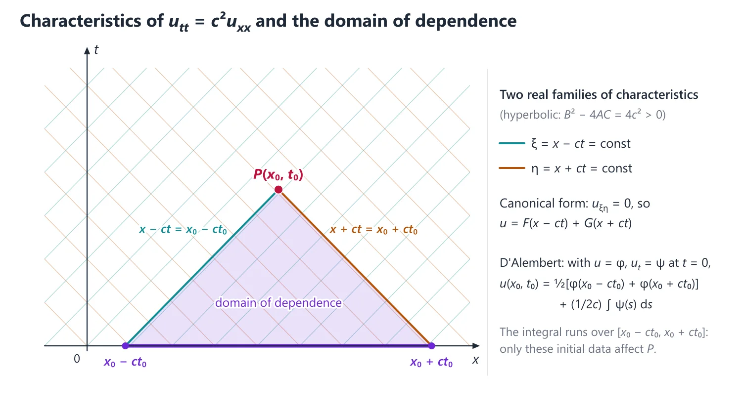
1. Understanding the Type of a Second-Order Equation
Why we need it: second-order equations behave in three very different ways: waves travel (hyperbolic), heat spreads and smooths (parabolic), and steady states settle (elliptic). Each type has its own canonical form and its own kind of boundary data, so the first question about any such equation is 'which type?'.
In words: only the second-order part A uxx + B uxy + C uyy decides the type; first-order terms, u itself and the right side never matter. A, B, C are the full coefficients as written (B is not halved).
The discriminant B2 − 4AC is computed at each point: positive means hyperbolic, zero parabolic, negative elliptic (hyperbolic, parabolic, elliptic). When A, B, C depend on x and y the sign, and hence the type, can change from one region to another.
First example, slowly: classify uxx + 2yuxy + xuyy = 0 in the whole plane.
Step 1: read the coefficients: A = 1 (of uxx), B = 2y (of uxy), C = x (of uyy).
Step 2: B2 − 4AC = 4y2 − 4x = 4(y2 − x).
Step 3: find where it vanishes: on the parabola x = y2, which divides the plane into two regions.
Step 4: test one point on each side: at (0, 1) the value is 4 > 0, and at (1, 0) it is −4 < 0.
Step 5: conclusion: hyperbolic where x < y2, parabolic on x = y2, elliptic where x > y2 (inside the parabola).
Step 6: notice that adding terms such as 5ux − u would not change any of this.
Non-example: in uuxx + uyy = 0 the coefficient A = u depends on the unknown solution, so B2 − 4AC = −4u cannot be evaluated from the equation alone: the type is known only once u is (elliptic where u > 0, hyperbolic where u < 0). The test as stated needs A, B, C to be functions of x and y only.
Building up: the type does not depend on the coordinates: under ξ = ξ(x, y), η = η(x, y) with Jacobian J ≠ 0 the new discriminant is J2(B2 − 4AC), and J2 > 0 (see 'Why it works' under Classification below).
This is why the names come from conics: AX2 + BXY + CY2 = 1 is a hyperbola, parabola or ellipse by the same sign, and a change of axes cannot turn one kind of conic into another.
Where it is used: 'classify the equation in different regions' questions, the type of a PDE just formed by elimination (Example 10 of the first topic), and the choice of canonical form in the next two lessons.
2. Understanding Characteristic Curves of a Second-Order Equation
Why we need it: to simplify A uxx + B uxy + C uyy we change to new variables ξ, η. The best choice makes the coefficient of uξξ (and if possible of uηη) vanish, and the curves ξ = constant that do this are the characteristics.
In words: the new coefficient of uξξ is A′ = Aξx2 + Bξxξy + Cξy2. On a level curve ξ = c the slope is dy/dx = −ξx/ξy, so A′ = 0 becomes A(dy/dx)2 − B(dy/dx) + C = 0.
So: solve this quadratic for the slope λ = dy/dx, integrate each ODE dy/dx = λ, and write the result as ξ(x, y) = constant. Two real slopes give two families, one double slope gives one family, and complex slopes give complex characteristics.
First example, slowly: find the characteristics of 3uxx + 10uxy + 3uyy = 0.
Step 1: A = 3, B = 10, C = 3 and B2 − 4AC = 100 − 36 = 64 > 0: hyperbolic, so expect two real families.
Step 2: the characteristic equation is 3λ2 − 10λ + 3 = 0, that is (3λ − 1)(λ − 3) = 0, so λ = 3 or λ = 1/3.
Step 3: dy/dx = 3 integrates to y − 3x = c, so ξ = y − 3x.
Step 4: dy/dx = 1/3 integrates to 3y − x = c, so η = 3y − x.
Step 5: check A′ for ξ: ξx = −3, ξy = 1 give 3(9) + 10(−3)(1) + 3(1) = 27 − 30 + 3 = 0.
Step 6: check for η: ηx = −1, ηy = 3 give 3(1) + 10(−1)(3) + 3(9) = 0. Both families are characteristic.
Step 7: the Jacobian ξxηy − ξyηx = (−3)(3) − (1)(−1) = −8 ≠ 0, so (ξ, η) is a genuine change of variables.
Non-example: with the wrong sign, 3λ2 + 10λ + 3 = 0 gives λ = −3, −1/3 and ξ = y + 3x. Then A′ = 3(9) + 10(3)(1) + 3(1) = 60 ≠ 0, so uξξ survives. The condition that fails is the minus sign in A(dy/dx)2 − B(dy/dx) + C = 0.
Building up: the same calculation with η in place of ξ gives C′, so for a hyperbolic equation both A′ and C′ vanish when ξ and η come from the two roots; for a parabolic one only one family exists; for an elliptic one the roots are complex conjugates (next lesson).
For the wave equation utt = c2uxx the characteristics are x ± ct = constant, the paths along which signals travel (see 'Why the minus sign' under Classification below for the derivation of the sign).
Where it is used: every reduction to canonical form, D'Alembert's solution of the wave equation, and the domain of dependence of hyperbolic problems.
3. Understanding the Reduction to Canonical Form
Why we need it: in the right variables a hyperbolic equation becomes uξη = (lower-order terms), a parabolic one uηη = (...), and an elliptic one uαα + uββ = (...). These canonical forms are easier to recognise and are often integrable, which is why UPSC asks 'reduce to canonical form and hence solve'.
In words: write u(x, y) = U(ξ, η). By the chain rule ux = ξxUξ + ηxUη and uy = ξyUξ + ηyUη; differentiating again gives uxx, uxy, uyy. Substitute, collect the coefficients of Uξξ, Uξη, Uηη, and divide by the surviving one.
With constant coefficients the second derivatives of ξ, η are zero, so no first-order terms appear; with variable coefficients terms such as ξxxUξ remain and form the right side.
First example, slowly: reduce 3uxx + 10uxy + 3uyy = 0 with ξ = y − 3x, η = 3y − x (previous lesson) and solve it.
Step 1: first derivatives: ux = −3Uξ − Uη and uy = Uξ + 3Uη.
Step 2: uxx = 9Uξξ + 6Uξη + Uηη (apply ∂/∂x = −3∂/∂ξ − ∂/∂η to ux).
Step 3: uxy = −3Uξξ − 10Uξη − 3Uηη (apply ∂/∂y = ∂/∂ξ + 3∂/∂η to ux), and uyy = Uξξ + 6Uξη + 9Uηη.
Step 4: collect: Uξξ has 27 − 30 + 3 = 0, Uηη has 3 − 30 + 27 = 0, and Uξη has 18 − 100 + 18 = −64.
Step 5: so −64Uξη = 0, and the canonical form is Uξη = 0. (Check: B′2 = 642 equals J2(B2 − 4AC) = 64 × 64.)
Step 6: integrate in η: Uξ = F′(ξ); then in ξ: U = F(ξ) + G(η).
Step 7: return to x, y: u = F(y − 3x) + G(3y − x), with F, G arbitrary.
Non-example: keeping ξ = y − 3x but taking η = 2y − 6x is not allowed: η = 2ξ, the Jacobian is 0, and u would be expressed through one variable only, so uξ and uη cannot be told apart. The condition that fails is J ≠ 0.
Building up: in matrix form the coefficients transform as M′ = JmMJmT ('Derivation: How the Coefficients Transform' below). For a parabolic equation take ξ from the single family and any η with J ≠ 0 (often η = x); then A′ = B′ = 0 and only Uηη survives.
For an elliptic equation with complex characteristic ξ = α + iβ, use the real variables α and β; then the coefficients of Uαα and Uββ become equal and Uαβ disappears, giving the Laplacian.
Where it is used: the 15–20 mark 'reduce to canonical form and hence solve' questions (Examples 7 to 12 below), and D'Alembert's solution, which is exactly Uξη = 0 for the wave equation.
4. Classification
General form: A uxx + B uxy + C uyy + F(x, y, u, ux, uy) = 0, where A, B, C are functions of x, y, not all zero.
At a point: B2 − 4AC > 0 hyperbolic, B2 − 4AC = 0 parabolic, B2 − 4AC < 0 elliptic.
Idea: the names come from conics: replacing uxx, uxy, uyy by X2, XY, Y2 gives AX2 + BXY + CY2, a hyperbola, parabola or ellipse by the same discriminant. The type also predicts behaviour: hyperbolic equations carry waves at finite speed along characteristics, parabolic ones diffuse and smooth, and elliptic ones describe equilibria in which every boundary point influences every interior point.
Under ξ = ξ(x, y), η = η(x, y) with Jacobian J = ξxηy − ξyηx ≠ 0, the new coefficients satisfy B′2 − 4A′C′ = J2(B2 − 4AC), so the type is invariant.
Why it works: write the principal part as the matrix M = [[A, B/2], [B/2, C]], so B2 − 4AC = −4 det M. The chain rule (Section 6) shows M′ = JmMJmT with Jm = [[ξx, ξy], [ηx, ηy]], hence det M′ = J2 det M; since J2 > 0 the sign, and so the type, cannot change.
New coefficients: A′ = Aξx2 + Bξxξy + Cξy2, B′ = 2Aξxηx + B(ξxηy + ξyηx) + 2Cξyηy, C′ = Aηx2 + Bηxηy + Cηy2.
Characteristic equation: A(dy)2 − B dx dy + C(dx)2 = 0, that is, A(dy/dx)2 − B(dy/dx) + C = 0.
Choosing ξ = constant along a characteristic makes A′ = 0, which is the basis of the reduction.
Why the minus sign: A′ = Aξx2 + Bξxξy + Cξy2 = 0; divide by ξy2 and use the slope of a level curve ξ = c, dy/dx = −ξx/ξy. Then ξx/ξy = −dy/dx and A(dy/dx)2 − B(dy/dx) + C = 0, which is the characteristic equation.
5. Reduction to Canonical Form
Hyperbolic: two real families of characteristics ξ(x, y) = c1, η(x, y) = c2; canonical form uξη = φ(ξ, η, u, uξ, uη), or uαα − uββ = ψ with α = ξ + η, β = ξ − η.
Parabolic: one family ξ(x, y) = c; take η any function with ∂(ξ, η)/∂(x, y) ≠ 0 (often η = x or y); canonical form uηη = φ(ξ, η, u, uξ, uη).
Why it works: by invariance B′2 − 4A′C′ = 0, and A′ = 0 then forces B′ = 0 as well; only C′uηη survives among the second derivatives, and C′ ≠ 0 because the Jacobian is non-zero.
Elliptic: complex conjugate characteristics ξ = α + iβ; take α = Re ξ, β = Im ξ; canonical form uαα + uββ = φ(α, β, u, uα, uβ).
Why it works: with Q(X, Y) = AX2 + BXY + CY2, the condition Q(∇ξ) = 0 for ξ = α + iβ splits into real and imaginary parts: Q(∇α) = Q(∇β) and the mixed term vanishes. These are exactly 'coefficient of uαα = coefficient of uββ' and 'no uαβ term'.
Constant coefficients: if λ1, λ2 are roots of Aλ2 − Bλ + C = 0, the characteristics are the straight lines y − λ1x = c1, y − λ2x = c2.
Idea: for the wave equation utt = c2uxx the characteristics are x ± ct = constant; the two through a point (x0, t0) cut the initial line at x0 ± ct0 and bound its domain of dependence (see the figure above). Data outside that interval cannot affect u(x0, t0).
6. Derivation: How the Coefficients Transform
With ux = ξxuξ + ηxuη and uy = ξyuξ + ηyuη, the second-order parts are uxx ~ ξx2uξξ + 2ξxηxuξη + ηx2uηη, uxy ~ ξxξyuξξ + (ξxηy + ξyηx)uξη + ηxηyuηη, uyy ~ ξy2uξξ + 2ξyηyuξη + ηy2uηη (~ means 'apart from first-order terms').
Multiplying by A, B, C and collecting uξξ, uξη, uηη gives exactly the A′, B′, C′ of Section 4; in matrix form M′ = JmMJmT.
Hyperbolic reduction: take ξ and η from the two real roots of the characteristic equation; then A′ = C′ = 0, and B′ ≠ 0 because B′2 = J2(B2 − 4AC) > 0. Dividing the transformed equation by B′ leaves uξη = φ.
The second form follows from α = ξ + η, β = ξ − η, since then uξη = uαα − uββ.
7. Choosing the Method
If A, B, C are constants → solve Aλ2 − Bλ + C = 0; the characteristics are y − λx = constant, and for complex λ = p ± iq take α = y − px, β = qx.
If the coefficients vary but the characteristic equation separates (such as y2dy2 = x2dx2) → take square roots and integrate each factor separately.
If A = 0 → x = constant is one family; if C = 0 → y = constant is one family.
If the equation is parabolic → ξ from the double root, η = x or y (whichever keeps J ≠ 0).
If the question asks for the type 'in different regions' → factor B2 − 4AC, find the curve where it vanishes (that curve is the parabolic set) and test one point on each side.
8. Common Mistakes
Plus sign in the characteristic equation: it is A(dy/dx)2 − B(dy/dx) + C = 0, as derived above; the plus sign replaces every slope λ by −λ, so both families come out wrong whenever B ≠ 0.
Mixing conventions: some books write 2B uxy and test B2 − AC; using B2 − 4AC with their B misclassifies uxx + 2uxy + uyy = 0 (B = 1 would give −3, 'elliptic', but the equation is parabolic).
Type at one point only: with variable coefficients give the type in every region, including the dividing curve, which is parabolic.
A singular change of variables: ξ = x + y with η = 2x + 2y has J = 0 and is not allowed; always show J ≠ 0.
Dropping first-order terms: with variable ξ, η the terms ξxxuξ, ηyyuη survive and give the right side of the canonical form (Example 2).
Link: the test is the classification of the conic AX2 + BXY + CY2 (Analytic Geometry); in n variables the type is read from the signs of the eigenvalues of the coefficient matrix, exactly as in the reduction of conicoids (Linear Algebra).
Link: the characteristics x ± ct = constant of the wave equation are the paths of D'Alembert's travelling waves f(x − ct), g(x + ct) (Vibrating String topic); a kink in the initial data travels along them and is never smoothed out, unlike in the heat equation.
9. Worked Examples
Example 1 (parabolic): uxx + 2uxy + uyy = 0. B2 − 4AC = 4 − 4 = 0; dy/dx = 1, so ξ = y − x; take η = x.
Then ux = −uξ + uη, uy = uξ, and uxx + 2uxy + uyy = uηη = 0.
Hence u = f(ξ) + ηg(ξ) = f(y − x) + xg(y − x).
Example 2 (hyperbolic): uxx − x2uyy = 0, x ≠ 0. B2 − 4AC = 4x2 > 0.
(dy/dx)2 = x2 gives ξ = y + x2/2, η = y − x2/2.
Then ux = x(uξ − uη), uxx = (uξ − uη) + x2(uξξ − 2uξη + uηη), uyy = uξξ + 2uξη + uηη.
So (uξ − uη) − 4x2uξη = 0; with x2 = ξ − η the canonical form is uξη = (uξ − uη)/(4(ξ − η)).
Example 3 (elliptic): uxx + x2uyy = 0, x ≠ 0. (dy/dx)2 = −x2 gives y ± ix2/2 = c, so α = y, β = x2/2.
Then ux = xuβ, uxx = uβ + x2uββ, uyy = uαα, so x2(uαα + uββ) + uβ = 0 and uαα + uββ = −uβ/(2β).
Example 4 (hyperbolic, variable coefficients): Reduce y2uxx − x2uyy = 0 (x, y > 0) to canonical form.
B2 − 4AC = 4x2y2 > 0; y2(dy/dx)2 = x2 gives y dy = ±x dx, so ξ = y2 − x2, η = y2 + x2.
ux = 2x(uη − uξ), uy = 2y(uξ + uη); substituting, y2uxx − x2uyy = −16x2y2uξη + 2ξuη − 2ηuξ.
Since 4x2y2 = η2 − ξ2, the canonical form is uξη = (ξuη − ηuξ)/(2(η2 − ξ2)).
Example 5 (elliptic, constant coefficients): Reduce uxx + 4uxy + 5uyy = 0 to canonical form.
B2 − 4AC = 16 − 20 = −4 < 0; λ2 − 4λ + 5 = 0 gives λ = 2 ± i, so the characteristics are y − (2 ± i)x = c; take α = y − 2x, β = x.
ux = −2uα + uβ, uy = uα; uxx = 4uαα − 4uαβ + uββ, uxy = −2uαα + uαβ, uyy = uαα.
Sum: (4 − 8 + 5)uαα + (−4 + 4)uαβ + uββ = 0, so the canonical form is uαα + uββ = 0.
Mixed type: the Tricomi equation yuxx + uyy = 0 is elliptic for y > 0, parabolic on y = 0 and hyperbolic for y < 0.
Standard types: the wave equation utt = c2uxx is hyperbolic, the heat equation ut = kuxx is parabolic, and the Laplace equation uxx + uyy = 0 is elliptic.
Example 6 (find all regions): Classify (1 − x2)uxx − 2xyuxy + (1 − y2)uyy = 0 at every point of the plane.
B2 − 4AC = 4x2y2 − 4(1 − x2)(1 − y2) = 4(x2 + y2 − 1).
So the equation is elliptic inside the unit circle x2 + y2 < 1, parabolic on x2 + y2 = 1 and hyperbolic outside it.
10. Choosing η and Integrating the Canonical Form
Parabolic: after ξ from the single characteristic, take η = x or η = y, whichever makes J = ξxηy − ξyηx ≠ 0; express the leftover coefficients in ξ, η.
Coefficient A = 0: the characteristic equation A dy2 − B dx dy + C dx2 = 0 then has the factor dx, so x = constant is one family of characteristics.
Chain rule in full: uxx = ξx2uξξ + 2ξxηxuξη + ηx2uηη + ξxxuξ + ηxxuη (similarly uxy, uyy); the terms ξxxuξ, ηxxuη produce the first-order part of the canonical form.
Solving the canonical form: uηη = g(η) integrates twice in η with 'constants' f(ξ), g(ξ); ηuηη + uη = 0 is ∂(ηuη)/∂η = 0; uξη + uη/ξ = 0 is ∂(ξuη)/∂ξ = 0; an equation of the form (∂y + α)(∂x + β)u = 0 is solved by putting w = ux + βu.
11. Past UPSC Questions Solved
Example 7 (UPSC 2015, 15 marks): Reduce the second-order partial differential equation x2 ∂2u/∂x2 − 2xy ∂2u/∂x∂y + y2 ∂2u/∂y2 + x ∂u/∂x + y ∂u/∂y = 0 into canonical form. Hence, find its general solution.
A = x2, B = −2xy, C = y2: B2 − 4AC = 0, parabolic; the characteristic equation is (x dy/dx + y)2 = 0, so ξ = xy; take η = x (J = −x ≠ 0).
ux = yuξ + uη, uy = xuξ, uxx = y2uξξ + 2yuξη + uηη, uxy = uξ + xyuξξ + xuξη, uyy = x2uξξ.
Second-order part = x2uηη − 2xyuξ; first-order part xux + yuy = 2xyuξ + xuη; the sum is x2uηη + xuη = 0.
Canonical form ηuηη + uη = 0, i.e. ∂(ηuη)/∂η = 0, so ηuη = f(ξ) and u = f(ξ)log η + g(ξ).
Answer: canonical form uηη = −(1/η)uη with ξ = xy, η = x; general solution u = f(xy)log x + g(xy).
Example 8 (UPSC 2017, 15 marks): Reduce the equation
y2 ∂2z/∂x2 − 2xy ∂2z/∂x∂y + x2 ∂2z/∂y2 = (y2/x) ∂z/∂x + (x2/y) ∂z/∂y
to canonical form and hence solve it.
A = y2, B = −2xy, C = x2: B2 − 4AC = 0, parabolic; (y dy/dx + x)2 = 0 gives ξ = x2 + y2; take η = x.
zx = 2xzξ + zη, zy = 2yzξ, zxx = 2zξ + 4x2zξξ + 4xzξη + zηη, zxy = 4xyzξξ + 2yzξη, zyy = 2zξ + 4y2zξξ.
LHS = 2(x2 + y2)zξ + y2zηη (the zξξ, zξη terms cancel); RHS = (y2/x)(2xzξ + zη) + (x2/y)(2yzξ) = 2(x2 + y2)zξ + (y2/x)zη.
So zηη = zη/η (with η = x2 instead, this becomes zηη = 0); then ∂(zη/η)/∂η = 0, zη = ηf(ξ) and z = (η2/2)f(ξ) + g(ξ).
Answer: canonical form zηη = (1/η)zη (ξ = x2 + y2, η = x); solution z = x2f(x2 + y2) + g(x2 + y2).
Example 9 (UPSC 2019, 20 marks): Reduce the following second order partial differential equation to canonical form and find the general solution :
∂2u/∂x2 − 2x ∂2u/∂x∂y + x2 ∂2u/∂y2 = ∂u/∂y + 12x.
A = 1, B = −2x, C = x2: B2 − 4AC = 0, parabolic; (dy/dx + x)2 = 0 gives ξ = y + x2/2; take η = x.
ux = xuξ + uη, uy = uξ, uxx = uξ + x2uξξ + 2xuξη + uηη, uxy = xuξξ + uξη, uyy = uξξ.
LHS = uξ + uηη, so uξ + uηη = uξ + 12x: canonical form uηη = 12η.
Integrating twice in η: u = 2η3 + ηf(ξ) + g(ξ).
Answer: u = 2x3 + xf(y + x2/2) + g(y + x2/2).
Example 10 (UPSC 2022, 15 marks): Reduce the following partial differential equation to a canonical form and hence solve it: yuxx + (x + y)uxy + xuyy = 0
A = y, B = x + y, C = x: B2 − 4AC = (x − y)2 > 0 for x ≠ y, hyperbolic; y(dy/dx)2 − (x + y)dy/dx + x = (y dy/dx − x)(dy/dx − 1) = 0 gives ξ = y − x, η = y2 − x2.
ux = −uξ − 2xuη, uy = uξ + 2yuη; uxx = uξξ + 4xuξη + 4x2uηη − 2uη, uxy = −uξξ − 2(x + y)uξη − 4xyuηη, uyy = uξξ + 4yuξη + 4y2uηη + 2uη.
Substituting, the uξξ and uηη coefficients vanish, uξη gets 8xy − 2(x + y)2 = −2(x − y)2 and uη gets 2(x − y).
With x − y = −ξ: canonical form uξη + (1/ξ)uη = 0, i.e. ∂(ξuη)/∂ξ = 0, so ξuη = F′(η) and u = F(η)/ξ + G(ξ).
Answer: uξη = −uη/ξ (ξ = y − x, η = y2 − x2); u = F(y2 − x2)/(y − x) + G(y − x). UPSC 2026 (Q6a) set the same equation.
Example 11 (UPSC 2023, 15 marks): Reduce the partial differential equation ∂2z/∂y2 − ∂2z/∂x∂y + ∂z/∂x − (∂z/∂y)(1 + 1/x) + z/x = 0 to canonical form.
Coefficients: A = 0 (zxx), B = −1 (zxy), C = 1 (zyy), so B2 − 4AC = 1 > 0, hyperbolic everywhere.
Characteristics: A dy2 − B dx dy + C dx2 = dx(dy + dx) = 0, so ξ = x, η = x + y.
zx = zξ + zη, zy = zη, zxy = zξη + zηη, zyy = zηη; substituting, zηη − zξη − zηη + zξ + zη − zη(1 + 1/ξ) + z/ξ = 0.
So zξη = zξ − (1/ξ)(zη − z); it factorises as (∂/∂ξ + 1/ξ)(zη − z) = 0, which gives z = ex + yG(x) + H(x + y)/x.
Answer: canonical form ∂2z/∂ξ∂η = ∂z/∂ξ − (1/ξ)(∂z/∂η − z) with ξ = x, η = x + y; general solution z = ex + yG(x) + H(x + y)/x.
Example 12 (UPSC 2024, 15 marks): Solve the partial differential equation
∂/∂y (∂φ/∂x + φ) + 2x2y (∂φ/∂x + φ) = 0
by transforming it to the canonical form.
Expanded: φxy + φy + 2x2yφx + 2x2yφ = 0; A = C = 0, B = 1, so B2 − 4AC = 1 > 0 (hyperbolic) and the characteristics are x = const, y = const.
With ξ = x, η = y the equation is already canonical: φξη = −φη − 2ξ2η(φξ + φ).
Put w = φx + φ: wy + 2x2yw = 0, so w = f(x)e−x2y2.
Then ∂(exφ)/∂x = exf(x)e−x2y2; integrate in x from a fixed x0.
Answer: φ(x, y) = e−x[g(y) + ∫x0x f(s)es − s2y2 ds], f and g arbitrary.
12. Practice Exercises
Exercise 1 (basic): Classify uxx + 4uxy + 4uyy = 0.
Answer: B2 − 4AC = 16 − 16 = 0: parabolic everywhere.
Exercise 2 (basic): Classify uxx + uxy + uyy = 0.
Answer: B2 − 4AC = 1 − 4 = −3 < 0: elliptic everywhere.
Exercise 3 (basic): Classify uxx − yuyy = 0.
Answer: B2 − 4AC = 4y: hyperbolic for y > 0, parabolic on y = 0, elliptic for y < 0.
Exercise 4 (standard): Reduce x2uxx − y2uyy = 0 (x, y > 0) to canonical form.
Answer: x2λ2 = y2 gives ξ = xy, η = y/x; the canonical form is uξη = uη/(2ξ).
Exercise 5 (standard): Reduce uxx + 2uxy + 5uyy = 0 to canonical form.
Answer: λ2 − 2λ + 5 = 0 gives λ = 1 ± 2i; with α = y − x, β = 2x the equation becomes 4(uαα + uββ) = 0, i.e. uαα + uββ = 0.
Exercise 6 (standard): Reduce uxx − 2uxy + uyy = 0 to canonical form and solve it.
Answer: parabolic, λ = −1 (double): ξ = x + y, η = x give uηη = 0, so u = f(x + y) + xg(x + y).
Exercise 7 (standard): Reduce uxx + 5uxy + 6uyy = 0 to canonical form and solve it.
Answer: λ = 2, 3: ξ = y − 2x, η = y − 3x give uξη = 0, so u = f(y − 2x) + g(y − 3x).
Exercise 8 (UPSC level): Reduce y2uxx + x2uyy = 0 (x, y > 0) to canonical form.
Answer: elliptic; y dy = ±ix dx gives α = y2, β = x2, and the canonical form is uαα + uββ = −uα/(2α) − uβ/(2β).
Exercise 9 (UPSC level): Reduce uxx − 2 sin x uxy − cos2x uyy − cos x uy = 0 to canonical form and find its general solution.
Answer: B2 − 4AC = 4 > 0; λ = −sin x ± 1 gives ξ = y + x − cos x, η = y − x − cos x; the first-order terms cancel and uξη = 0, so u = f(y + x − cos x) + g(y − x − cos x).
Exercise 10 (UPSC level): Reduce 4uxx + 12uxy + 9uyy = 9 to canonical form and find its general solution.
Answer: parabolic, λ = 3/2 (double): ξ = 2y − 3x, η = x give 4uηη = 9, so u = 9x2/8 + xf(2y − 3x) + g(2y − 3x).
| Type | B2 − 4AC | Characteristics | Canonical form | Prototype |
|---|---|---|---|---|
| Hyperbolic | > 0 | Two real families | uξη = φ | Wave equation |
| Parabolic | = 0 | One real family | uηη = φ | Heat equation |
| Elliptic | < 0 | Complex conjugate pair | uαα + uββ = φ | Laplace equation |
Mains points
- 'Classify and reduce to canonical form' is a staple 15-mark question, often with variable coefficients such as x2uxx − y2uyy = 0; state the region where each type holds.
- Show the characteristic equation, the new variables, the Jacobian ≠ 0 check, and all the chain-rule derivatives before substituting.
- Express leftover x, y in the final form in terms of ξ, η; examiners deduct marks for a mixed-variable answer.
- If asked to 'hence solve', integrate the canonical form (for example uξη = 0 gives u = f(ξ) + g(η)) and return to x, y.
- Common mistake: writing the characteristic equation as A(dy/dx)2 + B(dy/dx) + C = 0; the middle sign must be minus.
Did you know?
- The names come from conics: A x2 + B xy + C y2 = 1 is a hyperbola, parabola or ellipse exactly when B2 − 4AC is positive, zero or negative.
Vibrating String, Heat Equation and Laplace Equation
The three classical equations are solved on bounded domains by separation of variables: assume a product solution, obtain an eigenvalue problem from the boundary conditions, and fit the initial or boundary data by a Fourier series. The vibrating string utt = c2uxx gives oscillating modes (and D'Alembert's solution on an infinite string), the heat equation ut = kuxx gives exponentially decaying modes, and the Laplace equation gives sinh or rn modes.
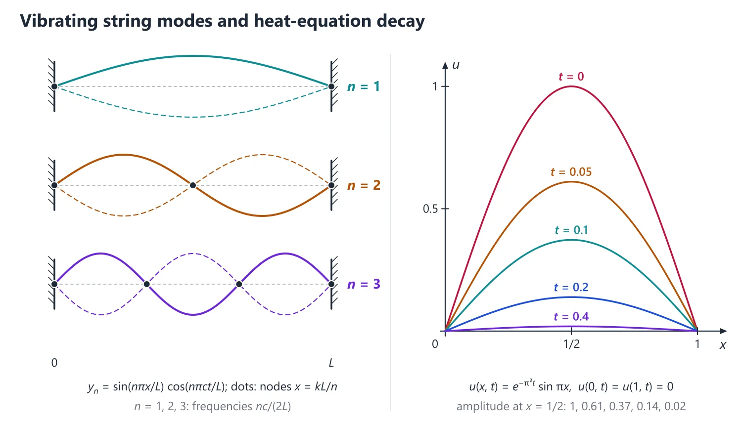
1. Understanding Separation of Variables and the Eigenvalue Problem
Why we need it: the heat, wave and Laplace equations on a bounded interval come with boundary conditions such as 'the ends are kept at 0'. General solutions with arbitrary functions are of little help there; we need a method that builds the boundary conditions in from the start.
In words: try a product u = X(x)T(t), one factor for each variable. For ut = kuxx this gives XT′ = kX″T, and dividing by kXT gives T′/(kT) = X″/X.
The left side depends only on t and the right side only on x; they can be equal for all x and t only if both equal one constant, written −λ (the separation constant).
The boundary conditions u(0, t) = u(L, t) = 0 become X(0) = X(L) = 0. The problem X″ + λX = 0 with these end values has non-zero solutions only for special λ, the eigenvalues, and these solutions are the eigenfunctions.
First example, slowly: solve ut = 2uxx, 0 < x < 1, u(0, t) = u(1, t) = 0, u(x, 0) = 5 sin 3πx.
Step 1: with u = X(x)T(t): T′/(2T) = X″/X = −λ, so X″ + λX = 0 and T′ = −2λT.
Step 2: the ends give X(0) = X(1) = 0 (otherwise T ≡ 0 and u ≡ 0).
Step 3: λ ≤ 0 gives only X = 0 (the case analysis is in 'Why it works' under Separation of Variables below). For λ = k2 > 0, X = A cos kx + B sin kx; X(0) = 0 gives A = 0, and X(1) = 0 gives sin k = 0, so k = nπ.
Step 4: so the eigenvalues are λn = n2π2 and the eigenfunctions are sin nπx, n = 1, 2, 3, ...
Step 5: the time factor is T = e−2n2π2t, so each mode is e−2n2π2tsin nπx.
Step 6: the initial data is already one mode, n = 3 with coefficient 5, so u = 5e−18π2tsin 3πx.
Step 7: check: ut = −18π2u and 2uxx = 2(−9π2)u = −18π2u; both ends give 0, and t = 0 gives 5 sin 3πx.
Non-example: if one end is held at u(0, t) = 1, a product would need X(0)T(t) = 1 for all t, which forces T to be constant and destroys the time dependence. Separation needs homogeneous boundary conditions; with non-zero end values, first subtract the steady state (see 'Ends at fixed non-zero temperatures' below).
Building up: the same separation for utt = c2uxx gives T″ + c2λT = 0, so the modes oscillate as cos(nπct/L) and sin(nπct/L); for Laplace's equation the second factor becomes sinh or cosh. General initial data are handled by adding modes, the subject of the next lesson.
Where it is used: every vibrating-string, heat-conduction and steady-plate question, and, through the eigenvalue idea, the Fourier series of Real Analysis and the eigenvectors of Linear Algebra.
2. Understanding Fitting the Initial Data by a Fourier Series
Why we need it: real initial data, such as a constant temperature or a plucked shape, is not a single sine. We must write it as a sum of the eigenfunctions so that each piece can be evolved separately.
In words: because the PDE and the boundary conditions are linear and homogeneous, any sum of modes u = ∑bne−kn2π2t/L2sin(nπx/L) is again a solution (superposition).
At t = 0 this must equal f(x): f(x) = ∑bnsin(nπx/L), a Fourier sine series. The coefficients are picked out by orthogonality: ∫0L sin(mπx/L)sin(nπx/L) dx is 0 for m ≠ n and L/2 for m = n.
So multiplying both sides by sin(mπx/L) and integrating kills every term except one, and bm = (2/L)∫0L f(x)sin(mπx/L) dx.
First example, slowly: solve ut = uxx, 0 < x < π, u(0, t) = u(π, t) = 0, u(x, 0) = π − x.
Step 1: here L = π and k = 1, so the modes are e−n2tsin nx and u = ∑bne−n2tsin nx.
Step 2: at t = 0 we need π − x = ∑bnsin nx on 0 < x < π, so bn = (2/π)∫0π(π − x)sin nx dx.
Step 3: integrate by parts, differentiating π − x and integrating sin nx: the integral is [−(π − x)cos nx/n]0π − ∫0π cos nx/n dx.
Step 4: the bracket is 0 − (−π/n) = π/n, and the last integral is sin nx/n2 from 0 to π, which is 0. So the integral is π/n.
Step 5: hence bn = (2/π)(π/n) = 2/n for every n.
Step 6: u(x, t) = 2∑n=1∞ (1/n)e−n2tsin nx.
Step 7: notice what the formula says: the higher modes die fastest, so for large t, u ≈ 2e−tsin x, a single arch shrinking to 0. (At x = 0 the series gives 0, not π: the data jump there, and the series takes the mean of the end values of the odd extension.)
Non-example: expanding π − x in a cosine series instead would give terms cos nx, which are not zero at x = 0 and x = π, so the boundary conditions u(0, t) = u(π, t) = 0 would fail. The eigenfunctions must be those of the boundary conditions: sines for fixed ends, cosines (with the constant term) for insulated ends.
Building up: for the wave equation there are two data, u(x, 0) = f and ut(x, 0) = g; f fixes the cosine-in-time coefficients An, and g fixes Bn with the extra factor L/(nπc) (see 'Why Bn has the factor 1/(nπc)' below).
The series converges to f wherever f is smooth, and to the average of the one-sided limits at a jump; the 'Useful integrals' below save time in the exam.
Where it is used: the 15–20 mark rod and string questions with data such as x, x(L − x), a constant or a triangle (Examples 5, 8, 9, 12 and 13 below).
3. Understanding D'Alembert's Solution of the Wave Equation
Why we need it: on a very long string (the whole line) there are no ends and no eigenvalues. D'Alembert's formula gives the solution in closed form and shows what the wave equation really does: it moves shapes.
In words: the characteristics of utt = c2uxx are x + ct = constant and x − ct = constant, and the general solution is F(x + ct) + G(x − ct): one shape moving left and one moving right, both with speed c and without change of form.
Fitting the initial displacement f and velocity g gives u = [f(x + ct) + f(x − ct)]/2 + (1/(2c))∫x − ctx + ct g(s) ds. The value at (x, t) depends only on the data in [x − ct, x + ct], the domain of dependence.
First example, slowly: solve utt = uxx on −∞ < x < ∞ with u(x, 0) = 1/(1 + x2) and ut(x, 0) = 0.
Step 1: identify c = 1, f(x) = 1/(1 + x2) (a single bump of height 1 at x = 0) and g = 0 (released from rest).
Step 2: since g = 0 the integral term vanishes, so u = [f(x + t) + f(x − t)]/2.
Step 3: substitute: u = (1/2)[1/(1 + (x + t)2) + 1/(1 + (x − t)2)].
Step 4: check t = 0: u = (1/2)(2f(x)) = f(x). Check ut at t = 0: it is [f′(x) − f′(x)]/2 = 0.
Step 5: interpret: the bump splits into two bumps of height 1/2; at t = 3 they are centred at x = 3 and x = −3.
Step 6: a sample value: u(0, 1) = (1/2)(1/2 + 1/2) = 1/2.
Step 7: with a non-zero velocity, for example g(x) = cos x and c = 1, the extra term is (1/2)∫x − tx + t cos s ds = (1/2)[sin(x + t) − sin(x − t)] = cos x sin t.
Non-example: on a finite string 0 < x < L with fixed ends the formula cannot be used as it stands, because x ± ct soon leaves (0, L) where f and g are given. The condition that fails is that the domain is the whole line; the remedy is to extend f and g as odd, 2L-periodic functions, which reproduces the Fourier series solution.
Building up: in characteristic variables ξ = x + ct, η = x − ct the equation becomes uξη = 0, so u = F(ξ) + G(η); the two data then fix F and G up to a constant that cancels ('Derivation: The Three Equations and D'Alembert's Formula' below).
Where it is used: infinite-string questions, checking separated solutions (sin x sin ct = [cos(x − ct) − cos(x + ct)]/2 is a pair of travelling waves), and the finite speed of propagation that distinguishes waves from heat.
4. Understanding Laplace's Equation on a Rectangle and a Disc
Why we need it: after a long time a heated plate reaches a steady state, ut = 0, and its temperature satisfies uxx + uyy = 0 with given values on the whole boundary. There is no time variable, so the role of time is taken by the second space variable.
In words: separate u = X(x)Y(y) to get X″/X = −Y″/Y = constant. Choose the sign so that the factor oscillates (sin) in the direction in which both boundary values are zero; the other factor is then sinh or cosh, chosen to vanish on the remaining zero side.
For a disc use polar coordinates: the angular factor must be 2π-periodic (cos nθ, sin nθ), and the radial factor rn is kept while r−n and log r are dropped because u must stay finite at the centre.
First example, slowly: solve uxx + uyy = 0 in the square 0 < x < π, 0 < y < π with u = 0 on x = 0, x = π and y = π, and u(x, 0) = sin 2x.
Step 1: the two zero sides x = 0 and x = π face each other, so X must oscillate: X″ + n2X = 0 with X(0) = X(π) = 0 gives X = sin nx.
Step 2: then Y″ = n2Y, and Y must vanish on the third zero side y = π; the combination that does this is Y = sinh(n(π − y)).
Step 3: so u = ∑cnsin nx sinh(n(π − y)); at y = 0 this is ∑cnsinh(nπ)sin nx, which must equal sin 2x.
Step 4: only n = 2 survives, with c2sinh 2π = 1.
Step 5: u = sin 2x sinh(2(π − y))/sinh 2π.
Step 6: check: uxx = −4u and uyy = 4u add to 0; x = 0 and x = π give 0, y = π gives sinh 0 = 0, and y = 0 gives sin 2x.
Step 7: notice that the temperature decays away from the heated side y = 0, roughly like e−2y.
Non-example: with the other sign, X″ = k2X gives X = A cosh kx + B sinh kx, and X(0) = 0, X(π) = 0 force A = 0 and B sinh kπ = 0, so X ≡ 0. The condition that fails is that the oscillating factor must be the one with two zero boundary values.
Building up: if several sides carry non-zero data, solve one problem per side and add (linearity). In a disc the same separation gives (r/a)n(ancos nθ + bnsin nθ) with an, bn the Fourier coefficients of the boundary data.
The centre value is then a0/2, the mean of the boundary values, and the maximum principle shows that the solution is unique ('Maximum principle' below).
Where it is used: steady temperatures in plates and discs, the annulus question of UPSC 2018 (Example 11 below), and potential problems in Fluid Dynamics and Complex Analysis, where harmonic functions are real parts of analytic functions.
5. Separation of Variables
Assume u = X(x)T(t), substitute, divide by XT and set both sides equal to a separation constant −λ.
Idea: after dividing, one side depends only on x and the other only on t; a function of x can equal a function of t for all x and t only if both are the same constant. The method needs linear homogeneous boundary conditions on the x-boundaries, so that each product term satisfies them separately.
With X(0) = X(L) = 0, the problem X″ + λX = 0 has eigenvalues λn = n2π2/L2 and eigenfunctions sin(nπx/L), n = 1, 2, 3, ...; λ ≤ 0 gives only X = 0.
Why it works: for λ = 0, X = A + Bx and X(0) = X(L) = 0 give A = B = 0; for λ = −k2 < 0, X = A cosh kx + B sinh kx, X(0) = 0 gives A = 0 and B sinh kL = 0 gives B = 0. For λ = k2 > 0, X = A cos kx + B sin kx, so A = 0 and sin kL = 0, i.e. k = nπ/L.
Superpose the product solutions and find the coefficients from the initial data using Fourier sine (or cosine) series.
Idea: superposition is allowed because the PDE and the boundary conditions are linear and homogeneous. The coefficients are picked out by orthogonality: ∫0L sin(mπx/L) sin(nπx/L) dx = 0 for m ≠ n and L/2 for m = n, so multiplying the series by sin(mπx/L) and integrating isolates one coefficient.
6. Vibrating String (Wave Equation)
utt = c2uxx, 0 < x < L, with c2 = T/ρ (tension over mass per unit length); u(0, t) = u(L, t) = 0, u(x, 0) = f(x), ut(x, 0) = g(x).
Solution: u = ∑n=1∞ [Ancos(nπct/L) + Bnsin(nπct/L)] sin(nπx/L).
An = (2/L)∫0L f(x) sin(nπx/L) dx, Bn = (2/(nπc))∫0L g(x) sin(nπx/L) dx.
The n-th normal mode has frequency nc/(2L); the fundamental frequency is c/(2L).
Idea: the n-th mode sin(nπx/L) has n − 1 interior nodes and vibrates at n times the fundamental frequency (see the figure above); this is why a string sounds a note with harmonics. Plucking at a node of mode n leaves that mode out (Section 9).
D'Alembert's solution (infinite string): u = [f(x + ct) + f(x − ct)]/2 + (1/(2c))∫x − ctx + ct g(s) ds.
Example 1: utt = uxx, 0 < x < π, fixed ends, u(x, 0) = 0, ut(x, 0) = sin 2x. Only B2 ≠ 0 and 2B2 = 1, so u = (1/2)sin 2t sin 2x.
Example 2: string released from rest with f(x) = kx(L − x): An = 8kL2/(n3π3) for odd n and 0 for even n, Bn = 0.
Example 3: Solve utt = c2uxx, −∞ < x < ∞, with u(x, 0) = x2, ut(x, 0) = sin x.
By D'Alembert: u = [(x + ct)2 + (x − ct)2]/2 + (1/(2c))∫x − ctx + ct sin s ds = x2 + c2t2 + (1/(2c))[cos(x − ct) − cos(x + ct)].
So u = x2 + c2t2 + (1/c)sin x sin ct (check: utt = 2c2 − c sin x sin ct = c2uxx).
7. Heat Equation
ut = kuxx (k the diffusivity), 0 < x < L, u(0, t) = u(L, t) = 0, u(x, 0) = f(x).
Idea: mode n decays like e−kn2π2t/L2, so the higher modes, which carry the sharp corners of f, die out first; the temperature profile smooths quickly and soon looks like the single arch sin(πx/L) shrinking to zero (see the figure above). Unlike the wave equation, time cannot be run backwards.
Solution: u = ∑ bn e−kn2π2t/L2 sin(nπx/L), with bn = (2/L)∫0L f(x) sin(nπx/L) dx.
Insulated ends (ux = 0 at x = 0, L): u = a0/2 + ∑ an e−kn2π2t/L2 cos(nπx/L), an = (2/L)∫0L f(x) cos(nπx/L) dx; u tends to the mean initial temperature a0/2.
Ends at fixed non-zero temperatures u(0, t) = T1, u(L, t) = T2: write u = T1 + (T2 − T1)x/L + v, where v solves the problem with zero end values.
Why it works: w(x) = T1 + (T2 − T1)x/L satisfies w″ = 0 and the end conditions, so it is the steady state; v = u − w then has zero end values and initial data f(x) − w(x), which must be expanded in the sine series.
Example 4: ut = uxx, 0 < x < π, u(0, t) = u(π, t) = 0, u(x, 0) = 3 sin x + 2 sin 3x. Then u = 3e−tsin x + 2e−9tsin 3x.
Example 5: A rod 0 ≤ x ≤ L has initial temperature 100 throughout, and both ends are kept at 0 for t > 0; find u(x, t) for ut = kuxx.
bn = (2/L)∫0L 100 sin(nπx/L) dx = (200/(nπ))(1 − cos nπ), which is 400/(nπ) for odd n and 0 for even n.
u = (400/π)∑n odd (1/n)e−kn2π2t/L2 sin(nπx/L), which tends to 0 as t → ∞.
8. Laplace Equation
uxx + uyy = 0 describes steady temperature and potential; its solutions are harmonic functions.
Idea: a harmonic function equals the average of its values on any circle centred at a point (mean value property), so it can have no interior peak or pit; it is the shape of a soap film or a stretched membrane fixed along a wire frame.
Rectangle 0 < x < a, 0 < y < b, with u = 0 on x = 0, x = a, y = 0 and u(x, b) = f(x): u = ∑ cn sin(nπx/a) sinh(nπy/a), where cn sinh(nπb/a) = (2/a)∫0a f(x) sin(nπx/a) dx.
Idea: choose the sign of the separation constant so that the factor oscillates (sin) in the direction with two zero boundary conditions; the other factor is then sinh or cosh, and sinh(nπy/a) is the one vanishing at y = 0. If the non-zero data are on y = 0 instead, use sinh(nπ(b − y)/a).
Example 6: f(x) = sin(πx/a) gives u = sin(πx/a) sinh(πy/a)/sinh(πb/a).
Disc r < R in polar form urr + ur/r + uθθ/r2 = 0 with u(R, θ) = f(θ): u = a0/2 + ∑ (r/R)n(ancos nθ + bnsin nθ), where an, bn are the Fourier coefficients of f.
Terms r−n and log r are discarded inside the disc because u must stay bounded at r = 0.
Example 7: Solve urr + ur/r + uθθ/r2 = 0 in r < 1 with u(1, θ) = cos2θ.
cos2θ = 1/2 + (1/2)cos 2θ, so a0/2 = 1/2, a2 = 1/2 and all other coefficients vanish.
u = 1/2 + (r2/2)cos 2θ = (1 + x2 − y2)/2; the value 1/2 at the centre is the mean of the boundary values.
Maximum principle: a function harmonic in a bounded domain and continuous on its closure attains its maximum and minimum on the boundary, and if it is non-constant, only there; hence the Dirichlet problem has at most one solution.
Why it works: if u1, u2 solve the same Dirichlet problem, w = u1 − u2 is harmonic and zero on the boundary; its maximum and minimum are both 0, so w ≡ 0.
9. Plucked Strings, Decay Terms and Useful Integrals
String plucked at x = a to height h and released from rest: An = 2hL2sin(nπa/L)/(n2π2a(L − a)), Bn = 0; modes with sin(nπa/L) = 0 are absent.
Decay term: ut = kuxx − γu becomes the heat equation for v under u = e−γtv, with the same boundary and initial data.
Useful integrals on 0 to L: ∫x sin(nπx/L) dx = (−1)n+1L2/(nπ); ∫sin(nπx/L) dx = L(1 − (−1)n)/(nπ); ∫x(L − x)sin(nπx/L) dx = 2L3(1 − (−1)n)/(n3π3); and ∫01 x2sin nπx dx = (−1)n+1/(nπ) + 2((−1)n − 1)/(nπ)3.
Data not vanishing at the ends (such as u(x, 0) = x): the formulas are unchanged; the sine series converges to the data in 0 < x < L but not at x = L, and a remark on this earns credit.
10. Laplace Equation in Polar Coordinates: Disc and Annulus
Separation: V = R(r)Θ(θ) gives Θ″ + n2Θ = 0 and r2R″ + rR′ − n2R = 0 (an Euler equation); 2π-periodicity in θ makes n = 0, 1, 2, ...
R = Anrn + Bnr−n for n ≥ 1 and A0 + B0log r for n = 0; Θ = cos nθ, sin nθ (or e±inθ).
Disc r ≤ a: drop r−n and log r (boundedness at r = 0); exterior r ≥ a: drop rn and log r (boundedness at ∞).
Annulus a ≤ r ≤ b: keep both powers and log r, expand both boundary functions in Fourier series, and solve a 2 × 2 system for each n; with u(a, θ) = 0 the radial factor is (r/a)n − (a/r)n.
11. Infinite Domains and Uniqueness
Fourier transform: F(k) = ∫−∞∞ f(x)e−ikx dx, f(x) = (1/(2π))∫−∞∞ F(k)eikx dk; f″ transforms to −k2F when f, f′ → 0 at ±∞, and the transform of a convolution ∫f(ξ)g(x − ξ) dξ is F(k)G(k).
Green's first identity: ∬S (w∇2w + |∇w|2) dx dy = ∮Γ w ∂w/∂n ds; it proves uniqueness for the Dirichlet problem (w = 0 on Γ) and, up to a constant, for the Neumann problem (∂w/∂n = 0 on Γ).
12. Derivation: The Three Equations and D'Alembert's Formula
Wave equation: take the piece of string between x and x + δx under tension T, with small slope ux. The net vertical force is T[ux(x + δx, t) − ux(x, t)] ≈ Tuxxδx, and Newton's law gives ρδx utt = Tuxxδx, so utt = c2uxx with c2 = T/ρ.
Heat equation: Fourier's law makes the heat flux −κux; the heat gained by a slab of width δx per unit time is κ[ux(x + δx) − ux(x)] ≈ κuxxδx, and this equals cρδx ut (c the specific heat, ρ the density), so ut = kuxx with k = κ/(cρ).
In the steady state ut = 0, and in two dimensions the same balance gives uxx + uyy = 0: Laplace's equation is the time-independent heat equation.
D'Alembert's formula: with ξ = x + ct, η = x − ct the wave equation becomes uξη = 0 (previous topic), so u = F(x + ct) + G(x − ct).
The data give F(x) + G(x) = f(x) and c[F′(x) − G′(x)] = g(x), so F(x) − G(x) = (1/c)∫0x g(s) ds + K.
Hence F = f/2 + (1/(2c))∫0x g + K/2 and G = f/2 − (1/(2c))∫0x g − K/2; adding F(x + ct) and G(x − ct), K cancels and the two integrals combine to (1/(2c))∫x − ctx + ct g(s) ds, which is the formula of Section 6.
Why Bn has the factor 1/(nπc): ut(x, 0) = ∑Bn(nπc/L) sin(nπx/L) = g(x), so Bn(nπc/L) = (2/L)∫g sin(nπx/L) dx, which gives Bn = (2/(nπc))∫0L g(x) sin(nπx/L) dx.
13. Choosing the Method
If the domain is the whole line → D'Alembert for the wave equation, the Fourier transform for the heat equation; if it is a finite interval → separation of variables.
If the ends are held at zero → sine series; if the ends are insulated → cosine series with the constant term; if the ends are at non-zero constants → subtract the steady state first.
If a rectangle has non-zero data on more than one side → split into one problem per side and add the solutions.
If the region is a disc, an annulus or the outside of a circle → polar coordinates with rn, r−n and log r, keeping only the bounded terms.
If the equation has an extra term −γu → put u = e−γtv first; if the data are already a finite sum of sines → read off the coefficients without integrating.
14. Common Mistakes
Non-zero end temperatures: expanding f itself in a sine series; it is f − w (initial data minus steady state) that has to be expanded.
Insulated ends: forgetting a0/2, which is the final temperature of the rod.
Wrong sinh factor: with data on y = 0 and u = 0 on y = b, the factor must vanish at y = b, so it is sinh(nπ(b − y)/a), not sinh(nπy/a).
Parity slips: 1 − cos nπ = 1 − (−1)n is 2 for odd n and 0 for even n; writing it as 2 for all n doubles the series.
Wrong limits in D'Alembert: the integral of g runs from x − ct to x + ct, not from 0 to x + ct.
Keeping unbounded terms: r−n and log r inside a disc, or rn outside it.
Link: the coefficients are Fourier series coefficients (Real Analysis), and the problem X″ + λX = 0, X(0) = X(L) = 0 is an eigenvalue problem like Ax = λx in Linear Algebra, with orthogonal eigenfunctions in place of orthogonal eigenvectors.
Link: harmonic functions are the real parts of analytic functions (Complex Analysis): the answer of Example 7, (1 + x2 − y2)/2, is Re((1 + z2)/2); the velocity potential of an irrotational incompressible flow also satisfies ∇2φ = 0 (Fluid Dynamics).
15. Past UPSC Questions Solved
Example 8 (UPSC 2014, 15 marks): Solve ∂2u/∂t2 = ∂2u/∂x2, 0 < x < 1, t > 0, given that
(i) u(x, 0) = 0, 0 ≤ x ≤ 1
(ii) ∂u/∂t (x, 0) = x2, 0 ≤ x ≤ 1
(iii) u(0, t) = u(1, t) = 0, for all t
Here c = 1, L = 1, u(x, 0) = 0, so An = 0 and u = ∑Bnsin nπt sin nπx with nπBn = 2∫01 x2sin nπx dx.
∫01 x2sin nπx dx = (−1)n+1/(nπ) + 2((−1)n − 1)/(nπ)3 (integrate by parts twice).
So Bn = (2/(n2π2))[(−1)n+1 + 2((−1)n − 1)/(n2π2)]: 2/(n2π2) − 8/(n4π4) for odd n and −2/(n2π2) for even n.
Answer: u(x, t) = ∑n=1∞ (2/(n2π2))[(−1)n+1 + 2((−1)n − 1)/(n2π2)] sin nπx sin nπt.
Example 9 (UPSC 2015, 15 marks): Find the solution of the initial-boundary value problem
ut − uxx + u = 0, 0 < x < l, t > 0
u(0, t) = u(l, t) = 0, t ≥ 0
u(x, 0) = x(l − x), 0 < x < l
Put u = e−tv: ut − uxx + u = e−t(vt − vxx), so vt = vxx with v(0, t) = v(l, t) = 0, v(x, 0) = x(l − x).
v = ∑bne−n2π2t/l2sin(nπx/l) with bn = (2/l)∫0l x(l − x)sin(nπx/l) dx = 4l2(1 − (−1)n)/(n3π3).
So bn = 8l2/(n3π3) for odd n and 0 for even n.
Answer: u(x, t) = (8l2/π3)∑n odd (1/n3)e−(1 + n2π2/l2)tsin(nπx/l).
Example 10 (UPSC 2017, 10 marks): Let Γ be a closed curve in xy-plane and let S denote the region bounded by the curve Γ. Let
∂2w/∂x2 + ∂2w/∂y2 = f(x, y) ∀ (x, y) ∈ S.
If f is prescribed at each point (x, y) of S and w is prescribed on the boundary Γ of S, then prove that any solution w = w(x, y), satisfying these conditions, is unique.
Let w1, w2 be two solutions and w = w1 − w2; then ∇2w = f − f = 0 in S and w = 0 on Γ.
Green's first identity (the divergence theorem for w∇w): ∬S (w∇2w + wx2 + wy2) dx dy = ∮Γ w ∂w/∂n ds.
Both ∇2w = 0 in S and w = 0 on Γ, so ∬S (wx2 + wy2) dx dy = 0.
The integrand is continuous and non-negative, so wx = wy = 0 in S; w is constant, and continuity up to Γ, where w = 0, gives w ≡ 0 (alternatively, apply the maximum principle to the harmonic w).
Answer: w1 = w2 throughout S, so the solution is unique. Hence proved.
Example 11 (UPSC 2018, 20 marks): A thin annulus occupies the region 0 < a ≤ r ≤ b, 0 ≤ θ ≤ 2π. The faces are insulated. Along the inner edge the temperature is maintained at 0°, while along the outer edge the temperature is held at T = K cos(θ/2), where K is a constant. Determine the temperature distribution in the annulus.
Steady state: urr + ur/r + uθθ/r2 = 0 in a ≤ r ≤ b, with u(a, θ) = 0 and u(b, θ) = K cos(θ/2), 0 ≤ θ ≤ 2π.
Fourier coefficients of cos(θ/2) on (0, 2π): (1/π)∫02π cos(θ/2)cos nθ dθ = 0 for all n ≥ 0, and (1/π)∫02π cos(θ/2)sin nθ dθ = 8n/(π(4n2 − 1)).
So K cos(θ/2) = (8K/π)∑n=1∞ n sin nθ/(4n2 − 1) for 0 < θ < 2π, and only the sine terms are needed (no constant or log r term).
Separated solutions (Anrn + Bnr−n)sin nθ with Anan + Bna−n = 0 give the radial factor (r/a)n − (a/r)n; dividing by its value at r = b matches the outer edge.
Answer: u(r, θ) = (8K/π)∑n=1∞ [n/(4n2 − 1)] · [(r/a)n − (a/r)n]/[(b/a)n − (a/b)n] · sin nθ (across θ = 0 the boundary value jumps between −K and K, and the series gives the mean 0 there).
Example 12 (UPSC 2020, 20 marks): One end of a tightly stretched flexible thin string of length l is fixed at the origin and the other at x = l. It is plucked at x = l/3 so that it assumes initially the shape of a triangle of height h in the x-y plane. Find the displacement y at any distance x and at any time t after the string is released from rest. Take, (horizontal tension)/(mass per unit length) = c2.
Initial shape y(x, 0) = 3hx/l for 0 ≤ x ≤ l/3 and 3h(l − x)/(2l) for l/3 ≤ x ≤ l; the string starts from rest, so Bn = 0 and y = ∑Ansin(nπx/l)cos(nπct/l).
Integrating by parts on each piece, the terms at x = l/3 cancel and only the jump in slope (3h/l + 3h/(2l) = 9h/(2l)) survives: An = (2/l)(l/(nπ))2(9h/(2l))sin(nπ/3).
So An = (9h/(n2π2))sin(nπ/3), the plucked-string formula with a = l/3.
Answer: y(x, t) = (9h/π2)∑n=1∞ (1/n2)sin(nπ/3)sin(nπx/l)cos(nπct/l); the modes n = 3, 6, 9, ... are absent.
Example 13 (UPSC 2023, 20 marks): Solve the partial differential equation a2 ∂2u/∂x2 = ∂2u/∂t2, 0 < x < L, t > 0 subject to the conditions
u(0, t) = 0, u(L, t) = 0, t > 0
u(x, 0) = x, (∂u/∂t)t=0 = 1, 0 < x < L
u = ∑[Ancos(nπat/L) + Bnsin(nπat/L)]sin(nπx/L), with An = (2/L)∫0L x sin(nπx/L) dx = 2L(−1)n+1/(nπ).
(nπa/L)Bn = (2/L)∫0L sin(nπx/L) dx = 2(1 − (−1)n)/(nπ), so Bn = 4L/(n2π2a) for odd n and 0 for even n.
[The data u(x, 0) = x and ut(x, 0) = 1 do not vanish at x = L, so the series represents them only in 0 < x < L.]
Answer: u(x, t) = (2L/π)∑n=1∞ ((−1)n+1/n)cos(nπat/L)sin(nπx/L) + (4L/(π2a))∑n odd (1/n2)sin(nπat/L)sin(nπx/L).
Example 14 (UPSC 2024, 20 marks): Show that the solution of the two-dimensional Laplace's equation
∂2φ(x, y)/∂x2 + ∂2φ(x, y)/∂y2 = 0, x ∈ (−∞, ∞), y ≥ 0
subject to the boundary condition
φ(x, 0) = f(x), x ∈ (−∞, ∞),
along with φ(x, y) → 0 for |x| → ∞ and y → ∞ can be written in the form
φ(x, y) = (y/π) ∫−∞∞ f(ξ) dξ/[y2 + (x − ξ)2].
Take the Fourier transform in x: Φ(k, y) = ∫−∞∞ φ(x, y)e−ikx dx; since φ, φx → 0 as |x| → ∞, φxx transforms to −k2Φ and the PDE becomes Φyy − k2Φ = 0.
Φ = A(k)e−|k|y + B(k)e|k|y; φ → 0 as y → ∞ forces B = 0, and y = 0 gives A = F(k), the transform of f.
The inverse of e−|k|y is g(x, y) = (1/(2π))∫e−|k|yeikx dk = (1/(2π))[1/(y − ix) + 1/(y + ix)] = y/(π(x2 + y2)).
Since Φ = F(k) · e−|k|y, the convolution theorem gives φ(x, y) = ∫f(ξ)g(x − ξ, y) dξ.
Answer: φ(x, y) = (y/π)∫−∞∞ f(ξ) dξ/[y2 + (x − ξ)2], Poisson's integral for the half-plane. Hence proved.
Example 15 (UPSC 2026, 15 marks): Two-dimensional harmonic equation in plane polar coordinates (r, θ) takes the form:
∂2V/∂r2 + (1/r) ∂V/∂r + (1/r2) ∂2V/∂θ2 = 0
Deduce that it has solutions of the form (Arn + Br−n) e±inθ, where A, B, n are constants. Determine V if it satisfies the two-dimensional harmonic equation in the region 0 ≤ r ≤ a, 0 ≤ θ ≤ 2π and satisfies the conditions:
(i) V remains finite as r → 0,
(ii) V = ∑n cn cos(nθ) on r = a.
Put V = R(r)Θ(θ) and multiply by r2/(RΘ): (r2R″ + rR′)/R = −Θ″/Θ = n2 (a separation constant).
Θ″ + n2Θ = 0 gives Θ = e±inθ; r2R″ + rR′ − n2R = 0 is an Euler equation, and R = rm gives m2 = n2, so R = Arn + Br−n.
Hence V = (Arn + Br−n)e±inθ; single-valuedness makes n an integer (n = 0 gives A + B log r).
In 0 ≤ r ≤ a, finiteness at r = 0 forces B = 0 and removes log r, so V = ∑ rn(Ancos nθ + Bn′sin nθ); at r = a, Anan = cn and Bn′ = 0.
Answer: V(r, θ) = ∑n cn(r/a)ncos nθ.
16. Practice Exercises
Exercise 1 (basic): Find the eigenvalues and eigenfunctions of X″ + λX = 0, X(0) = 0, X′(L) = 0.
Answer: λn = ((2n − 1)π/(2L))2 and Xn = sin((2n − 1)πx/(2L)), n = 1, 2, 3, ... (λ ≤ 0 gives only X = 0).
Exercise 2 (basic): Solve ut = uxx, 0 < x < π, u(0, t) = u(π, t) = 0, u(x, 0) = 4 sin 2x − sin 5x.
Answer: u = 4e−4tsin 2x − e−25tsin 5x.
Exercise 3 (basic): Use D'Alembert's formula to solve utt = 4uxx on the whole line with u(x, 0) = 0, ut(x, 0) = 2x.
Answer: c = 2: u = (1/4)∫x − 2tx + 2t 2s ds = (1/4)[(x + 2t)2 − (x − 2t)2] = 2xt.
Exercise 4 (standard): A rod 0 ≤ x ≤ 2 with ut = 3uxx has its ends kept at 0 and initial temperature 5. Find u(x, t).
Answer: bn = ∫02 5 sin(nπx/2) dx = 10(1 − (−1)n)/(nπ), so u = (20/π)∑n odd (1/n)e−3n2π2t/4sin(nπx/2).
Exercise 5 (standard): Solve ut = uxx, 0 < x < π, with insulated ends ux(0, t) = ux(π, t) = 0 and u(x, 0) = cos2x.
Answer: cos2x = 1/2 + (1/2)cos 2x, so u = 1/2 + (1/2)e−4tcos 2x, which tends to the mean 1/2.
Exercise 6 (standard): A string 0 < x < π with c = 2 and fixed ends starts from u(x, 0) = 0 with velocity ut(x, 0) = sin x + 3 sin 2x. Find u.
Answer: u = ∑Bnsin 2nt sin nx with 2nBn equal to the coefficients of the data: u = (1/2)sin 2t sin x + (3/4)sin 4t sin 2x.
Exercise 7 (standard): Solve ut = uxx, 0 < x < 1, u(0, t) = 0, u(1, t) = 10, u(x, 0) = 10x + 3 sin 2πx.
Answer: the steady state is 10x and v = u − 10x starts from 3 sin 2πx, so u = 10x + 3e−4π2tsin 2πx.
Exercise 8 (UPSC level): Solve uxx + uyy = 0 in the rectangle 0 < x < a, 0 < y < b with u = 0 on x = 0, y = 0 and y = b, and u(a, y) = y(b − y).
Answer: u = ∑cnsinh(nπx/b)sin(nπy/b) with cnsinh(nπa/b) = 4b2(1 − (−1)n)/(n3π3); so u = (8b2/π3)∑n odd sinh(nπx/b)sin(nπy/b)/(n3sinh(nπa/b)).
Exercise 9 (UPSC level): Find the steady temperature in the annulus 1 ≤ r ≤ 2 when u(1, θ) = 0 and u(2, θ) = sin θ.
Answer: try u = (Ar + B/r)sin θ: A + B = 0 and 2A + B/2 = 1 give A = 2/3, B = −2/3, so u = (2/3)(r − 1/r)sin θ.
Exercise 10 (UPSC level): A string of length L with fixed ends is released from rest in the shape u(x, 0) = μ sin3(πx/L). Find the displacement.
Answer: sin3θ = (3 sin θ − sin 3θ)/4, so u = (μ/4)[3 sin(πx/L)cos(πct/L) − sin(3πx/L)cos(3πct/L)].
| Equation | Time or y factor | Coefficients |
|---|---|---|
| Wave utt = c2uxx | Ancos(nπct/L) + Bnsin(nπct/L) | An from f, Bn from g with factor L/(nπc) |
| Heat ut = kuxx | e−kn2π2t/L2 | bn = Fourier sine coefficients of f |
| Laplace uxx + uyy = 0 | sinh(nπy/L) (u = 0 on y = 0) | Fit u(x, b) and divide by sinh(nπb/L) |
| Form of the problem | Method | Watch out for |
|---|---|---|
| Wave, fixed ends | Sine series in x; cos and sin in t | Bn carries L/(nπc) |
| Wave, infinite string | D'Alembert's formula | Integral from x − ct to x + ct |
| Heat, ends at 0 | Sine series; e−kn2π2t/L2 | Odd/even n simplification |
| Heat, insulated ends | Cosine series | Keep a0/2 |
| Heat, ends at T1, T2 | Subtract the steady state | Expand f − w, not f |
| Laplace, rectangle | sin in the direction with two zero sides; sinh in the other | One problem per non-zero side |
| Laplace, disc or annulus | Polar Fourier series | Keep only bounded terms |
Mains points
- A full boundary-value problem (string with given initial displacement, rod with given initial temperature, or a rectangular plate) is asked almost every year for 15–20 marks.
- Show why the separation constant must be negative for non-trivial solutions (cases λ < 0, λ = 0, λ > 0), then the eigenvalues and eigenfunctions.
- Compute Fourier coefficients fully, including the odd/even simplification, and write the final series explicitly.
- For D'Alembert's solution, state the formula, substitute the data and simplify; questions sometimes ask for the displacement at a particular time.
- Common mistake: forgetting the factor 1/(nπc) in Bn for the wave equation, or using a cosine series where the boundary conditions require a sine series.
Did you know?
- Fourier developed his series in 1807 to solve the heat equation; the claim that 'any' function can be expanded in sines and cosines was so controversial that his memoir waited until 1822 to appear as a book.
Solved Problems: Partial Differential Equations
Fourteen UPSC-style problems with full solutions covering the whole chapter: formation of PDEs, Lagrange's method and integral surfaces, Charpit's method and the Cauchy problem, linear equations with constant coefficients, canonical forms, and boundary value problems for the wave, heat and Laplace equations. Each solution shows the steps an examiner looks for and ends with a boxed answer.
1. Formation of PDEs and Lagrange's Method
Problem 1 (10 marks): Form the partial differential equation by eliminating the arbitrary function φ from φ(x2 + y2 + z2, z2 − 2xy) = 0.
Let u = x2 + y2 + z2, v = z2 − 2xy; the eliminant is Pp + Qq = R with P = ∂(u, v)/∂(y, z), Q = ∂(u, v)/∂(z, x), R = ∂(u, v)/∂(x, y).
P = uyvz − uzvy = (2y)(2z) − (2z)(−2x) = 4z(x + y).
Q = uzvx − uxvz = (2z)(−2y) − (2x)(2z) = −4z(x + y).
R = uxvy − uyvx = (2x)(−2x) − (2y)(−2y) = 4(y2 − x2).
Dividing 4z(x + y)p − 4z(x + y)q = 4(y − x)(y + x) by 4(x + y) gives the equation.
Answer: z(p − q) = y − x.
Problem 2 (15 marks): Find the integral surface of (2xy − 1)p + (z − 2x2)q = 2(x − yz) which passes through the line x = 1, z = 0.
Multipliers x, y, 1/2: x(2xy − 1) + y(z − 2x2) + (x − yz) = 0, so x dx + y dy + dz/2 = 0 and x2 + y2 + z = c1.
Multipliers z, 1, x: z(2xy − 1) + (z − 2x2) + 2x(x − yz) = 0, so z dx + dy + x dz = 0 and xz + y = c2.
On the line x = 1, z = 0, y = t: c1 = 1 + t2 and c2 = t, so c1 = 1 + c22.
Replacing c1, c2: x2 + y2 + z = 1 + (xz + y)2, which simplifies to x2 + z − 1 = x2z2 + 2xyz.
Check: at x = 1, z = 0 both sides are 0 for every y, so the whole line lies on the surface.
Answer: x2 + y2 + z = 1 + (xz + y)2, that is x2(1 − z2) − 2xyz + z − 1 = 0.
2. Nonlinear First-Order Equations and the Cauchy Problem
Problem 3 (15 marks): Use Charpit's method to find a complete integral of px + qy = pq.
F = px + qy − pq: Fx = p, Fy = q, Fz = 0, Fp = x − q, Fq = y − p.
Charpit's equations include −dp/(Fx + pFz) = −dq/(Fy + qFz), that is dp/p = dq/q, so p = aq.
Substituting: aqx + qy = aq2, so q = (ax + y)/a and p = ax + y.
dz = (ax + y)dx + ((ax + y)/a)dy = (1/a)(ax + y)d(ax + y), so z = (ax + y)2/(2a) + b.
Check: px + qy = (ax + y)(x + y/a) = (ax + y)2/a = pq.
Answer: z = (ax + y)2/(2a) + b.
Problem 4 (10 marks): Find the complete and singular integrals of z = px + qy + √(1 + p2 + q2).
This is Clairaut's form, so the complete integral is z = ax + by + √(1 + a2 + b2).
Let S = √(1 + a2 + b2); differentiating with respect to a and b: x + a/S = 0 and y + b/S = 0.
So a = −xS, b = −yS, and x2 + y2 = (a2 + b2)/S2 = 1 − 1/S2.
Then z = −S(x2 + y2) + S = S(1 − x2 − y2) = 1/S = √(1 − x2 − y2), which satisfies the PDE (p = −x/z, q = −y/z).
Answer: complete integral z = ax + by + √(1 + a2 + b2); singular integral x2 + y2 + z2 = 1 (with z > 0).
Problem 5 (15 marks): Solve the Cauchy problem uux + uy = 1 with u = s/2 on the line x = y = s, and state where the solution fails.
Characteristic equations: dx/dt = u, dy/dt = 1, du/dt = 1, with x = y = s and u = s/2 at t = 0.
J = x0′b − y0′a = 1 · 1 − 1 · (s/2) = 1 − s/2, which is non-zero for s ≠ 2.
Solving: u = s/2 + t, y = s + t, x = s + st/2 + t2/2.
With t = y − s: x = s − sy/2 + y2/2, so s = (2x − y2)/(2 − y).
u = s/2 + t = y − s/2 = (4y − y2 − 2x)/(2(2 − y)); on x = y = s this gives (2s − s2)/(2(2 − s)) = s/2, as required.
Answer: u = (4y − y2 − 2x)/(2(2 − y)), valid for y ≠ 2; at the point s = 2 of the data line J = 0 (the line touches a characteristic projection), and the formula breaks down on y = 2.
3. Linear Equations with Constant Coefficients
Problem 6 (10 marks): Solve (D2 + DD′ − 6D′2)z = cos(2x + y).
Auxiliary m2 + m − 6 = 0 gives m = 2, −3: CF = φ1(y + 2x) + φ2(y − 3x).
The usual rule fails: D2 → −4, DD′ → −2, D′2 → −1 gives −4 − 2 + 6 = 0, because y + 2x is an argument of the CF.
PI = (D − 2D′)−1(D + 3D′)−1cos(2x + y); since (D + 3D′)sin(2x + y) = 5cos(2x + y), (D + 3D′)−1cos(2x + y) = (1/5)sin(2x + y).
By the failing-case rule, (D − 2D′)−1(1/5)sin(y + 2x) = (x/5)sin(y + 2x).
Check with w = 2x + y: zxx + zxy − 6zyy = [(4cos w − 4x sin w) + (cos w − 2x sin w) + 6x sin w]/5 = cos w.
Answer: z = φ1(y + 2x) + φ2(y − 3x) + (x/5)sin(2x + y).
Problem 7 (15 marks): Solve (D − D′ − 1)(D − D′ − 2)z = e2x − y + x.
Each factor has the form D − mD′ − c with m = 1 (c = 1 and c = 2), so CF = exφ1(y + x) + e2xφ2(y + x).
For e2x − y: D → 2, D′ → −1 gives (2 + 1 − 1)(2 + 1 − 2) = 2, so PI1 = (1/2)e2x − y.
For x, write E = D − D′: 1/((E − 1)(E − 2)) = (1/2)(1 − E)−1(1 − E/2)−1 = (1/2)(1 + (3/2)E + ...).
Since Ex = 1 and E2x = 0, PI2 = (1/2)(x + 3/2) = x/2 + 3/4.
Check: (E2 − 3E + 2)(x/2 + 3/4) = 0 − 3/2 + x + 3/2 = x.
Answer: z = exφ1(y + x) + e2xφ2(y + x) + (1/2)e2x − y + x/2 + 3/4.
4. Classification and Canonical Forms
Problem 8 (15 marks): Reduce uxx − 2uxy − 3uyy = 0 to canonical form, and solve it with u(x, 0) = 3x2, uy(x, 0) = 0.
B2 − 4AC = 4 + 12 = 16 > 0, so the equation is hyperbolic; λ2 + 2λ − 3 = 0 gives λ = 1, −3, so ξ = y − x, η = y + 3x.
ux = −uξ + 3uη, uy = uξ + uη; then uxx − 2uxy − 3uyy = −16uξη, so uξη = 0 and u = f(y − x) + g(y + 3x).
Data: f(−x) + g(3x) = 3x2 and f′(−x) + g′(3x) = 0; differentiating the first, −f′(−x) + 3g′(3x) = 6x.
Adding: 4g′(3x) = 6x, so g′(s) = s/2 and g(s) = s2/4 + C; then f′(r) = 3r/2 and f(r) = 3r2/4 − C.
u = (3/4)(y − x)2 + (1/4)(y + 3x)2 = 3x2 + y2; check: 6 − 0 − 3(2) = 0, u(x, 0) = 3x2, uy(x, 0) = 0.
Answer: canonical form uξη = 0 with ξ = y − x, η = y + 3x; u = 3x2 + y2.
Problem 9 (10 marks): Show that x2uxx + 2xyuxy + y2uyy = 0 is parabolic, reduce it to canonical form for x ≠ 0, and find its general solution.
B2 − 4AC = 4x2y2 − 4x2y2 = 0 at every point, so the equation is parabolic everywhere.
The characteristic equation x2(dy/dx)2 − 2xy(dy/dx) + y2 = 0, that is (x dy/dx − y)2 = 0, gives ξ = y/x; take η = x.
ux = −(y/x2)uξ + uη, uy = uξ/x, so the Euler operator E = x∂/∂x + y∂/∂y becomes η∂/∂η.
The given operator equals E2 − E = η2∂2/∂η2 + η∂/∂η − η∂/∂η = η2∂2/∂η2, so the equation becomes η2uηη = 0.
Integrating twice in η: u = f(ξ) + ηg(ξ).
Answer: canonical form uηη = 0 with ξ = y/x, η = x; general solution u = f(y/x) + xg(y/x).
5. Wave, Heat and Laplace Equations
Problem 10 (15 marks): A string of length L with fixed ends is pulled aside at its midpoint to a height h and released from rest. Find the displacement u(x, t).
Initial shape f(x) = 2hx/L for 0 ≤ x ≤ L/2 and f(x) = 2h(L − x)/L for L/2 ≤ x ≤ L; g(x) = 0, so Bn = 0.
An = (2/L)[∫0L/2 (2hx/L)sin(nπx/L) dx + ∫L/2L (2h(L − x)/L)sin(nπx/L) dx].
Integrating by parts, the terms in cos(nπ/2) cancel and the bracket equals (4hL/(n2π2))sin(nπ/2), so An = (8h/(n2π2))sin(nπ/2).
u = (8h/π2)∑n=1∞ (sin(nπ/2)/n2)sin(nπx/L)cos(nπct/L); only odd n appear, with alternating signs.
Answer: u(x, t) = (8h/π2)[sin(πx/L)cos(πct/L) − (1/9)sin(3πx/L)cos(3πct/L) + (1/25)sin(5πx/L)cos(5πct/L) − ...].
Problem 11 (15 marks): Solve ut = uxx, 0 < x < π, t > 0, with insulated ends ux(0, t) = ux(π, t) = 0 and u(x, 0) = x.
Separation with X′(0) = X′(π) = 0 gives X = cos nx, n = 0, 1, 2, ..., and T = e−n2t.
a0 = (2/π)∫0π x dx = π.
an = (2/π)∫0π x cos nx dx = (2/π)(cos nπ − 1)/n2, which is −4/(πn2) for odd n and 0 for even n ≥ 2.
So u = π/2 − (4/π)∑n odd e−n2tcos nx/n2.
Answer: u(x, t) = π/2 − (4/π)[e−tcos x + e−9tcos 3x/9 + e−25tcos 5x/25 + ...], which tends to the mean temperature π/2 as t → ∞.
Problem 12 (15 marks): Solve uxx + uyy = 0 in the square 0 < x < π, 0 < y < π, with u = 0 on x = 0, x = π and y = 0, and u(x, π) = x(π − x).
Separation with X(0) = X(π) = 0 gives X = sin nx and Y″ = n2Y; Y(0) = 0 gives Y = sinh ny, so u = ∑ cn sin nx sinh ny.
At y = π: cn sinh nπ = (2/π)∫0π x(π − x)sin nx dx = 4(1 − cos nπ)/(πn3).
So cn = 8/(πn3 sinh nπ) for odd n and cn = 0 for even n.
Answer: u(x, y) = (8/π)∑n odd sin nx sinh ny/(n3 sinh nπ).
Problem 13 (10 marks): Find the steady temperature u(r, θ) in the disc r < a when u(a, θ) = sin3θ, and the temperature at the centre.
sin3θ = (3 sin θ − sin 3θ)/4, so b1 = 3/4, b3 = −1/4 and all other Fourier coefficients are 0.
Each boundary term sin nθ extends to the bounded harmonic function (r/a)nsin nθ inside the disc.
At r = 0 the solution is 0, which equals the mean of sin3θ over a period (mean value property).
Answer: u(r, θ) = (3r/(4a))sin θ − (r3/(4a3))sin 3θ; u = 0 at the centre.
Problem 14 (10 marks): For utt = c2uxx, 0 < x < L, with u(0, t) = u(L, t) = 0, show that E(t) = (1/2)∫0L (ut2 + c2ux2) dx is constant, and deduce that the initial-boundary value problem has at most one smooth solution.
dE/dt = ∫0L (ututt + c2uxuxt) dx = c2∫0L (utuxx + uxuxt) dx = c2∫0L ∂(utux)/∂x dx.
This equals c2[utux]0L = 0, because u = 0 at both ends for all t gives ut(0, t) = ut(L, t) = 0.
If u1, u2 are two solutions with the same data, w = u1 − u2 solves the problem with zero data, so Ew(t) = Ew(0) = 0.
The integrand is continuous and non-negative, so wt = wx = 0; w is constant and w(0, t) = 0 gives w ≡ 0.
Answer: dE/dt = 0, so energy is conserved, and the solution is unique.
Mains points
- Integral surface through a curve, Charpit's method and the canonical form of a second-order equation are the most frequent 15-mark PDE questions; separation-of-variables problems (string, rod, rectangle) are the standard 15- or 20-mark items.
- In Lagrange problems, show the multipliers and verify lP + mQ + nR = 0 in one line; this is where the method marks are.
- In Cauchy problems, compute the Jacobian J on the data curve and say where it vanishes; examiners reward the existence-uniqueness remark.
- For particular integrals, test F(a, b) first and switch to the failing-case rule or the general method when it is 0, rather than forcing the shortcut.
- For Fourier-series solutions, write the separated ODEs, the eigenvalues, the coefficient integral and its evaluated value, then the final series with the first few terms written out.
Did you know?
- Problem 8 shows a useful check: when the data are polynomials, the solution of a constant-coefficient hyperbolic problem is often a polynomial too, here simply u = 3x2 + y2, which can be verified in one line.
UPSC Previous Year Questions: Partial Differential Equations
All 55 question parts (795 marks) on Partial Differential Equations asked in UPSC CSE Mathematics Optional papers from 2014–2026, transcribed from the official papers on upsc.gov.in and grouped by the topic in these notes that teaches them. The most heavily examined areas are Vibrating String, Heat Equation and Laplace Equation and Linear Second-Order PDEs with Constant Coefficients.
1. Families of Surfaces and Formation of PDEs
2024 Paper II, Q5(a), 10 marks: Show that if f and g are arbitrary functions of their respective arguments, then u = f(x − kt + iαy) + g(x − kt − iαy), is a solution of
∂2u/∂x2 + ∂2u/∂y2 = (1/C2) ∂2u/∂t2, where α2 = 1 − k2/C2.
2023 Paper II, Q5(a), 10 marks: By eliminating the arbitrary functions f and g from z = f(x2 − y) + g(x2 + y), form partial differential equation.
2022 Paper II, Q5(a), 10 marks: It is given that the equation of any cone with vertex at (a, b, c) is f((x − a)/(z − c), (y − b)/(z − c)) = 0. Find the differential equation of the cone.
2021 Paper II, Q5(a), 10 marks: Obtain the partial differential equation by eliminating arbitrary function f from the equation f(x + y + z, x2 + y2 + z2) = 0.
2020 Paper II, Q5(a), 10 marks: Form a partial differential equation by eliminating the arbitrary functions f(x) and g(y) from z = y f(x) + x g(y) and specify its nature (elliptic, hyperbolic or parabolic) in the region x > 0, y > 0.
2019 Paper II, Q5(a), 10 marks: Form a partial differential equation of the family of surfaces given by the following expression :
ψ(x2 + y2 + 2z2, y2 − 2zx) = 0.
2018 Paper II, Q5(a), 10 marks: Find the partial differential equation of the family of all tangent planes to the ellipsoid : x2 + 4y2 + 4z2 = 4, which are not perpendicular to the xy plane.
2. Lagrange's Method for Quasilinear First-Order PDEs
2026 Paper II, Q5(a), 10 marks: Find the integral surface of the equations dx/(xz − y) = dy/(yz − x) = dz/(1 − z2).
2024 Paper II, Q7(a), 15 marks: Find the integral surface of the following quasi-linear equation
(y − φ) ∂φ/∂x + (φ − x) ∂φ/∂y = x − y,
which passes through the curve φ = 0, xy = 1 and through the circle x + y + φ = 0, x2 + y2 + φ2 = a2.
2020 Paper II, Q6(a), 15 marks: Find the integral surface of the partial differential equation : (x − y)y2 ∂z/∂x + (y − x)x2 ∂z/∂y = (x2 + y2)z that contains the curve : xz = a3, y = 0 on it.
2018 Paper II, Q6(a), 15 marks: Find the general solution of the partial differential equation :
(y3x − 2x4)p + (2y4 − x3y)q = 9z(x3 − y3),
where p = ∂z/∂x, q = ∂z/∂y, and find its integral surface that passes through the curve : x = t, y = t2, z = 1.
2016 Paper II, Q5(a), 10 marks: Find the general equation of surfaces orthogonal to the family of spheres given by x2 + y2 + z2 = cz.
2016 Paper II, Q5(e), 10 marks: Find the general integral of the partial differential equation
(y + zx)p − (x + yz)q = x2 − y2.
2015 Paper II, Q5(a), 10 marks: Solve the partial differential equation (y2 + z2 − x2)p − 2xyq + 2xz = 0 where p = ∂z/∂x and q = ∂z/∂y.
2015 Paper II, Q6(a), 15 marks: Solve for the general solution p cos(x + y) + q sin(x + y) = z, where p = ∂z/∂x and q = ∂z/∂y.
3. Cauchy's Method of Characteristics and Nonlinear First-Order PDEs
2025 Paper II, Q7(a), 15 marks: Find the complete integral of z(p2 − q2) = x − y; p ≡ ∂z/∂x, q ≡ ∂z/∂y.
2025 Paper II, Q8(a), 15 marks: Find the characteristics of the partial differential equation
p2 + q2 = 2; p ≡ ∂z/∂x, q ≡ ∂z/∂y
and determine the integral surface which passes through x = 0, z = y.
2021 Paper II, Q8(a), 15 marks: Find a complete integral of the partial differential equation p = (z + qy)2 by using Charpit’s method.
2020 Paper II, Q7(a), 15 marks: Find the solution of the partial differential equation : z = (1/2)(p2 + q2) + (p − x)(q − y); p ≡ ∂z/∂x, q ≡ ∂z/∂y which passes through the x-axis.
2019 Paper II, Q6(a), 15 marks: Solve the first order quasilinear partial differential equation by the method of characteristics :
x ∂u/∂x + (u − x − y) ∂u/∂y = x + 2y in x > 0, −∞ < y < ∞ with u = 1 + y on x = 1.
2017 Paper II, Q6(a), 15 marks: Find a complete integral of the partial differential equation
2(pq + yp + qx) + x2 + y2 = 0.
2016 Paper II, Q6(a), 15 marks: Determine the characteristics of the equation z = p2 − q2, and find the integral surface which passes through the parabola 4z + x2 = 0, y = 0.
4. Linear Second-Order PDEs with Constant Coefficients
2026 Paper II, Q7(a), 15 marks: Solve the partial differential equation (2D2 − 5DD′ + 2D′2) z = 24(y − x) + sin(y − x), where D ≡ ∂/∂x, D′ ≡ ∂/∂y, z = z(x, y).
2025 Paper II, Q5(a), 10 marks: Find the solution of the equation (D2 + DD′ − 2D2) z = y sin x, where D ≡ ∂/∂x and D′ ≡ ∂/∂y.
2023 Paper II, Q6(a), 15 marks: Find the surface passing through the two lines z = x = 0 and z − 1 = x − y = 0, and satisfying the partial differential equation ∂2z/∂x2 − 4 ∂2z/∂x∂y + 4 ∂2z/∂y2 = 0.
2022 Paper II, Q7(a), 15 marks: Find the general solution of the partial differential equation (D2 + DD′ − 6D′2) z = x2 sin(x + y) where D ≡ ∂/∂x and D′ ≡ ∂/∂y.
2021 Paper II, Q7(a), 15 marks: Find the general solution of the partial differential equation (D2 − D′2 − 3D + 3D′)z = xy + ex+2y where D ≡ ∂/∂x and D′ ≡ ∂/∂y.
2020 Paper II, Q5(d), 10 marks: Solve the partial differential equation : (D3 − 2D2D′ − DD′2 + 2D′3)z = e2x+y + sin(x − 2y); D ≡ ∂/∂x, D′ ≡ ∂/∂y
2018 Paper II, Q7(a), 15 marks: Solve the partial differential equation :
(2D2 − 5DD′ + 2D′2)z = 5 sin(2x + y) + 24(y − x) + e3x + 4y
where D ≡ ∂/∂x, D′ ≡ ∂/∂y.
2017 Paper II, Q5(a), 10 marks: Solve (D2 − 2DD′ + D′2)z = ex+2y + x3 + sin 2x,
where D ≡ ∂/∂x, D′ ≡ ∂/∂y, D2 ≡ ∂2/∂x2, D′2 ≡ ∂2/∂y2.
2016 Paper II, Q7(a), 15 marks: Solve the partial differential equation
∂3z/∂x3 − 2 ∂3z/∂x2∂y − ∂3z/∂x∂y2 + 2 ∂3z/∂y3 = ex+y
2015 Paper II, Q5(b), 10 marks: Solve (D2 + DD′ − 2D′2)u = ex+y, where D = ∂/∂x and D′ = ∂/∂y.
2014 Paper II, Q5(a), 10 marks: Solve the partial differential equation (2D2 − 5DD′ + 2D′2)z = 24(y − x).
5. Classification and Canonical Forms of Second-Order PDEs
2026 Paper II, Q6(a), 20 marks: Reduce the partial differential equation y ∂2z/∂x2 + (x + y) ∂2z/∂x∂y + x ∂2z/∂y2 = 0 to canonical form and hence solve it.
2024 Paper II, Q8(a), 15 marks: Solve the partial differential equation
∂/∂y (∂φ/∂x + φ) + 2x2y (∂φ/∂x + φ) = 0
by transforming it to the canonical form.
2023 Paper II, Q8(a), 15 marks: Reduce the partial differential equation ∂2z/∂y2 − ∂2z/∂x∂y + ∂z/∂x − (∂z/∂y)(1 + 1/x) + z/x = 0 to canonical form.
2022 Paper II, Q8(a), 15 marks: Reduce the following partial differential equation to a canonical form and hence solve it: yuxx + (x + y)uxy + xuyy = 0
2019 Paper II, Q7(c), 20 marks: Reduce the following second order partial differential equation to canonical form and find the general solution :
∂2u/∂x2 − 2x ∂2u/∂x∂y + x2 ∂2u/∂y2 = ∂u/∂y + 12x.
2017 Paper II, Q7(a), 15 marks: Reduce the equation
y2 ∂2z/∂x2 − 2xy ∂2z/∂x∂y + x2 ∂2z/∂y2 = (y2/x) ∂z/∂x + (x2/y) ∂z/∂y
to canonical form and hence solve it.
2015 Paper II, Q8(a), 15 marks: Reduce the second-order partial differential equation x2 ∂2u/∂x2 − 2xy ∂2u/∂x∂y + y2 ∂2u/∂y2 + x ∂u/∂x + y ∂u/∂y = 0 into canonical form. Hence, find its general solution.
2014 Paper II, Q6(a), 15 marks: Reduce the equation ∂2z/∂x2 = x2 ∂2z/∂y2 to canonical form.
6. Vibrating String, Heat Equation and Laplace Equation
2026 Paper II, Q8(a), 15 marks: Two-dimensional harmonic equation in plane polar coordinates (r, θ) takes the form:
∂2V/∂r2 + (1/r) ∂V/∂r + (1/r2) ∂2V/∂θ2 = 0
Deduce that it has solutions of the form (Arn + Br−n) e±inθ, where A, B, n are constants. Determine V if it satisfies the two-dimensional harmonic equation in the region 0 ≤ r ≤ a, 0 ≤ θ ≤ 2π and satisfies the conditions:
(i) V remains finite as r → 0,
(ii) V = ∑n cn cos(nθ) on r = a.
2025 Paper II, Q6(a), 20 marks: Solve ∂2u/∂x2 + ∂2u/∂y2 = 0 for a rectangular plate subject to the boundary conditions
u(0, y) = 0, u(a, y) = 0
u(x, 0) = 0, u(x, b) = f(x)
2024 Paper II, Q6(a), 20 marks: Show that the solution of the two-dimensional Laplace's equation
∂2φ(x, y)/∂x2 + ∂2φ(x, y)/∂y2 = 0, x ∈ (−∞, ∞), y ≥ 0
subject to the boundary condition
φ(x, 0) = f(x), x ∈ (−∞, ∞),
along with φ(x, y) → 0 for |x| → ∞ and y → ∞ can be written in the form
φ(x, y) = (y/π) ∫−∞∞ f(ξ) dξ/[y2 + (x − ξ)2].
2023 Paper II, Q7(c), 20 marks: Solve the partial differential equation a2 ∂2u/∂x2 = ∂2u/∂t2, 0 < x < L, t > 0 subject to the conditions
u(0, t) = 0, u(L, t) = 0, t > 0
u(x, 0) = x, (∂u/∂t)t=0 = 1, 0 < x < L
2022 Paper II, Q6(a), 20 marks: Solve the heat equation ∂u/∂t = ∂2u/∂x2, 0 < x < l, t > 0 subject to the conditions
u(0, t) = u(l, t) = 0
u(x, 0) = x(l − x), 0 ≤ x ≤ l
2021 Paper II, Q6(a), 20 marks: Solve the wave equation a2 ∂2u/∂x2 = ∂2u/∂t2, 0 < x < L, t > 0 subject to the conditions u(0, t) = 0, u(L, t) = 0, u(x, 0) = (1/4)x(L − x), ∂u/∂t|t=0 = 0
2020 Paper II, Q8(a), 20 marks: One end of a tightly stretched flexible thin string of length l is fixed at the origin and the other at x = l. It is plucked at x = l/3 so that it assumes initially the shape of a triangle of height h in the x-y plane. Find the displacement y at any distance x and at any time t after the string is released from rest. Take, (horizontal tension)/(mass per unit length) = c2.
2018 Paper II, Q8(c), 20 marks: A thin annulus occupies the region 0 < a ≤ r ≤ b, 0 ≤ θ ≤ 2π. The faces are insulated. Along the inner edge the temperature is maintained at 0°, while along the outer edge the temperature is held at T = K cos(θ/2), where K is a constant. Determine the temperature distribution in the annulus.
2017 Paper II, Q5(d), 10 marks: Let Γ be a closed curve in xy-plane and let S denote the region bounded by the curve Γ. Let
∂2w/∂x2 + ∂2w/∂y2 = f(x, y) ∀ (x, y) ∈ S.
If f is prescribed at each point (x, y) of S and w is prescribed on the boundary Γ of S, then prove that any solution w = w(x, y), satisfying these conditions, is unique.
2017 Paper II, Q8(a), 20 marks: Given the one-dimensional wave equation
∂2y/∂t2 = c2 ∂2y/∂x2; t > 0,
where c2 = T/m, T is the constant tension in the string and m is the mass per unit length of the string.
(i) Find the appropriate solution of the above wave equation.
(ii) Find also the solution under the conditions
y(0, t) = 0, y(l, t) = 0 for all t
and [∂y/∂t]t=0 = 0, y(x, 0) = a sin(πx/l), 0 < x < l, a > 0.
2016 Paper II, Q8(a), 20 marks: Find the temperature u(x, t) in a bar of silver of length 10 cm and constant cross-section of area 1 cm2. Let density ρ = 10·6 g/cm3, thermal conductivity K = 1·04 cal/(cm sec °C) and specific heat σ = 0·056 cal/g °C. The bar is perfectly isolated laterally, with ends kept at 0°C and initial temperature f(x) = sin(0·1πx) °C. Note that u(x, t) follows the heat equation ut = c2uxx, where c2 = K/(ρσ).
2015 Paper II, Q7(a), 15 marks: Find the solution of the initial-boundary value problem
ut − uxx + u = 0, 0 < x < l, t > 0
u(0, t) = u(l, t) = 0, t ≥ 0
u(x, 0) = x(l − x), 0 < x < l
2014 Paper II, Q7(a), 15 marks: Find the deflection of a vibrating string (length = π, ends fixed, ∂2u/∂t2 = ∂2u/∂x2) corresponding to zero initial velocity and initial deflection f(x) = k(sin x − sin 2x).
2014 Paper II, Q8(a), 15 marks: Solve ∂2u/∂t2 = ∂2u/∂x2, 0 < x < 1, t > 0, given that
(i) u(x, 0) = 0, 0 ≤ x ≤ 1
(ii) ∂u/∂t (x, 0) = x2, 0 ≤ x ≤ 1
(iii) u(0, t) = u(1, t) = 0, for all t
| Topic | Parts asked | Total marks | Years |
|---|---|---|---|
| Families of Surfaces and Formation of PDEs | 7 | 70 | 2018, 2019, 2020, 2021, 2022, 2023, 2024 |
| Lagrange's Method for Quasilinear First-Order PDEs | 8 | 100 | 2015, 2016, 2018, 2020, 2024, 2026 |
| Cauchy's Method of Characteristics and Nonlinear First-Order PDEs | 7 | 105 | 2016, 2017, 2019, 2020, 2021, 2025 |
| Linear Second-Order PDEs with Constant Coefficients | 11 | 140 | 2014, 2015, 2016, 2017, 2018, 2020, 2021, 2022, 2023, 2025, 2026 |
| Classification and Canonical Forms of Second-Order PDEs | 8 | 130 | 2014, 2015, 2017, 2019, 2022, 2023, 2024, 2026 |
| Vibrating String, Heat Equation and Laplace Equation | 14 | 250 | 2014, 2015, 2016, 2017, 2018, 2020, 2021, 2022, 2023, 2024, 2025, 2026 |
Mains points
- Attempt each question here only after finishing the matching topic; time yourself at about 7 minutes per 10 marks.
- Questions repeat in idea, not wording: if a method appears in three or more years, practise it until it is routine.
- After solving, compare your method with the topic's worked examples and note any step you missed in your error log.
- Use the frequency table to prioritise revision in the last two months before the exam.
Mathematics Optional: All chapters
- Exam Pattern, Syllabus and Strategy
- Linear Algebra
- Calculus
- Analytic Geometry
- Ordinary Differential Equations
- Dynamics and Statics
- Vector Analysis
- Abstract Algebra
- Real Analysis
- Complex Analysis
- Linear Programming
- Partial Differential Equations
- Numerical Analysis and Computer Programming
- Mechanics and Fluid Dynamics