
Mathematics Optional · UPSC Notes
Ordinary Differential Equations — UPSC Maths Optional Notes
Free, exam-focused notes for UPSC Prelims and Mains, with Prelims tips and Mains points for every topic. 8 topics.
Open in the interactive reader: bookmarks, progress tracking and read-aloud.
Formulation and First Order, First Degree Equations
A family of curves with n arbitrary constants gives an ODE of order n. First order, first degree equations are solved by recognising the type: separable, homogeneous, linear, Bernoulli or exact. A non-exact equation M dx + N dy = 0 is made exact by an integrating factor found from a small set of standard rules.
1. Understanding Order, Degree and the Formation of an ODE
Why we need it: many laws of nature are statements about rates: a hot body cools at a rate proportional to its excess temperature, and a population grows at a rate proportional to its size. Such a law is a relation between an unknown function and its derivatives, that is, a differential equation. In the other direction, a geometric family of curves (all circles of radius 1, all lines through the origin) is described by an equation containing constants, and removing the constants gives the single rule that every member of the family obeys.
In words: an ordinary differential equation (ODE) connects one independent variable x, a dependent variable y and the derivatives dy/dx, d2y/dx2, ...; "ordinary" means there is only one independent variable, so no partial derivatives occur. The order is the order of the highest derivative that occurs. The degree is the power of that highest derivative once the equation has been written as a polynomial in all the derivatives.
A solution on an interval I is a function y(x) which, substituted together with its derivatives, makes the equation an identity for every x in I. A general solution of an n-th order equation contains n essential arbitrary constants (they cannot be merged into fewer); giving the constants numerical values gives a particular solution.
First example, slowly: find the ODE of all straight lines through the origin, y = mx with m arbitrary.
(1) There is one constant m, so we expect a first order equation. (2) Differentiate once: dy/dx = m. This still contains m, so on its own it describes only the lines of one particular slope.
(3) Eliminate m with the help of the original equation: m = y/x. (4) Substitute: dy/dx = y/x, that is x dy/dx − y = 0. (5) Check: every y = mx gives x·m − mx = 0. The equation has order 1, degree 1 and no constant: it is the rule shared by every line through the origin.
Non-example: y = A + B + x2 seems to have two constants, but A + B is a single constant C, so one differentiation already gives y′ = 2x, a first order equation; the constants were not essential. Similarly y″ + ey′ = 0 has order 2 but no degree, because ey′ is not a polynomial in y′; and √(y′) = x − y must be squared to (y′) = (x − y)2 before its degree (1) is read.
Building up: why exactly n differentiations? The family equation F(x, y, c1, ..., cn) = 0 and its first n derivatives are n + 1 equations; in general n of them can be solved for the n constants and the result substituted in the last one, leaving a relation between x, y, y′, ..., y(n) only. Fewer differentiations leave a constant behind; more give a higher order equation with extra, unwanted solutions.
The count also works backwards: an n-th order equation needs n initial conditions y(x0), y′(x0), ..., y(n−1)(x0) to single out one solution, one condition for each arbitrary constant (Picard's theorem, later in this topic, makes this precise for n = 1).
Where it is used: formation questions ("form the ODE of all circles", "of all ellipses with axes along the coordinate axes") are standard 10-mark items; the same elimination of the parameter is Step 1 of every orthogonal trajectory problem, and the order and degree decide which solution method applies.
2. Formulation of Differential Equations
Order is the order of the highest derivative present; degree is the power of the highest-order derivative after the equation is made free of radicals and fractions in the derivatives.
Idea: the degree is defined only when the equation is a polynomial in the derivatives. y′ + sin(y′) = x has order 1 but no degree; (y″)3/2 = 1 + y′ has degree 3, because squaring gives (y″)3 = (1 + y′)2.
A family of curves with n independent arbitrary constants gives an ODE of order n: differentiate n times and eliminate the n constants.
Why n derivatives: the curve equation and its first n derivatives give n + 1 equations, enough to eliminate n constants and leave one relation between x, y, y′, ..., y(n). The constants must be essential: y = Aex + B = (AeB)ex has only one, and gives the first order equation y′ = y.
Example 1: Form the ODE whose general solution is y = Ae2x + Be−3x.
y′ = 2Ae2x − 3Be−3x, y″ = 4Ae2x + 9Be−3x, so y″ + y′ − 6y = (4 + 2 − 6)Ae2x + (9 − 3 − 6)Be−3x = 0; the ODE is y″ + y′ − 6y = 0 (order 2, degree 1).
3. Understanding Separable and Homogeneous Equations
Why we need it: a first order, first degree equation dy/dx = f(x, y) prescribes a slope at every point, and solving it means finding the curves that follow these slopes. The easiest case is when the x-part and the y-part of f can be pulled apart, because then each side can be integrated by ordinary one-variable calculus.
In words: dy/dx = f(x, y) is separable if f(x, y) = g(x)h(y); then dy/h(y) = g(x) dx wherever h(y) ≠ 0. A function f(x, y) is homogeneous of degree n if f(tx, ty) = tnf(x, y) for all t > 0. If M and N are homogeneous of the same degree, dy/dx = M/N depends only on the ratio v = y/x, and the substitution y = vx turns it into a separable equation in v and x.
First example, slowly: solve dy/dx = (x + y)/x. (1) Test homogeneity: numerator and denominator both have degree 1, and dividing by x gives dy/dx = 1 + y/x, a function of y/x alone. (2) Put y = vx; by the product rule dy/dx = v + x dv/dx.
(3) Substitute: v + x dv/dx = 1 + v, so x dv/dx = 1. Notice that the term v cancels on both sides; this always happens, and it is what makes the equation separable. (4) Separate and integrate: dv = dx/x gives v = log|x| + c.
(5) Return to y: y/x = log|x| + c, that is y = x log|x| + cx. (6) Check: y′ = log|x| + 1 + c, and (x + y)/x = 1 + log|x| + c; the two agree, so the answer is right.
Non-example: dy/dx = (x + y + 1)/x is not homogeneous: replacing (x, y) by (tx, ty) gives (tx + ty + 1)/(tx), which is not a function of y/x alone because of the constant 1 (this one is linear instead). And dy/dx = sin(xy) is not separable, because sin(xy) cannot be written as g(x)h(y).
Building up: if M, N are homogeneous of degree n, then M(x, y) = xnM(1, y/x) and N(x, y) = xnN(1, y/x), so M/N = M(1, v)/N(1, v) = F(v). With y = vx this gives x dv/dx = F(v) − v, that is dv/(F(v) − v) = dx/x. If F(v0) = v0 for a constant v0, the line y = v0x is itself a solution which the division loses; check such lines separately.
Where it is used: the substitution y = vx returns in orthogonal trajectories (families of circles), in the reducible form (ax + by + c)/(a′x + b′y + c′) after shifting the origin, and behind Rule 3 for integrating factors.
4. Understanding Linear and Bernoulli Equations
Why we need it: many models are linear in the unknown: a tank with inflow q(t) and outflow proportional to the content, dy/dt + ky = q(t), or an electric circuit L di/dt + Ri = E(t). Separation fails as soon as a forcing term Q(x) is present, so we need a method that works for every continuous P and Q.
In words: dy/dx + P(x)y = Q(x) is linear: y and y′ occur only to the first power and are never multiplied together, and P, Q depend on x only. An integrating factor μ(x) is a multiplier chosen so that μ(y′ + Py) is the exact derivative (μy)′. Bernoulli's equation y′ + Py = Qyn is not linear because of yn, but it becomes linear in the new unknown z = y1−n.
First example, slowly: solve dy/dx + 2y = e−x. (1) Read P = 2 and Q = e−x; the coefficient of dy/dx is already 1. (2) IF = e∫2 dx = e2x; no constant is needed in the IF.
(3) Multiply: e2xy′ + 2e2xy = ex, and notice that the left side is (e2xy)′ by the product rule. (4) Integrate: e2xy = ex + c; the constant enters at this step. (5) Divide by e2x: y = e−x + ce−2x.
(6) Notice the structure of the answer: ce−2x is the general solution of y′ + 2y = 0, and e−x is one particular solution of the full equation. This "homogeneous part + one particular solution" pattern is the CF + PI of higher order linear equations.
Non-example: y′ + y2 = x is neither linear (because of y2) nor Bernoulli (the nonlinear term is not of the form Q(x)yn on the right of a linear left side); it is a Riccati equation and needs other methods. Also, x y′ + y = x2 is linear, but P must be read after dividing by x: P = 1/x, not 1.
Building up: the IF must satisfy μ′ = Pμ (derived in the section on the linear IF below), which gives μ = e∫P dx. For Bernoulli, dividing by yn gives y−ny′ + Py1−n = Q; with z = y1−n, z′ = (1 − n)y−ny′, so z′ + (1 − n)Pz = (1 − n)Q, a linear equation in z. For n > 0, y = 0 is also a solution and must be listed separately.
Where it is used: growth, decay and cooling problems, equations that are linear in x (dx/dy + P(y)x = Q(y)), the variation of parameters idea of the second order topic, and every IVP of the form y′ + Py = Q, y(x0) = y0.
5. Standard First Order, First Degree Types
Variables separable: f(x) dx = g(y) dy; integrate both sides.
Idea: separable means the slope factorises as (function of x) × (function of y). Dividing by g(y) can lose constant solutions: for dy/dx = y, dividing by y gives y = cex, and y = 0 is recovered only as c = 0; for dy/dx = √y the solution y = 0 is not of the form (x + c)2/4 at all.
Homogeneous: dy/dx = f(x, y)/g(x, y) with f, g homogeneous of the same degree; put y = vx, so dy/dx = v + x dv/dx and the variables separate.
Why it works: f/g homogeneous of degree 0 means it depends only on v = y/x, so the slope is the same at all points of a ray through the origin. Then x dv/dx = F(v) − v separates: dv/(F(v) − v) = dx/x.
Reducible to homogeneous: dy/dx = (ax + by + c)/(a′x + b′y + c′); if a/a′ ≠ b/b′ shift the origin by x = X + h, y = Y + k to remove the constants; if a/a′ = b/b′ put z = ax + by.
Why it works: if a/a′ ≠ b/b′ the lines ax + by + c = 0 and a′x + b′y + c′ = 0 meet at (h, k); moving the origin there removes the constants and leaves a homogeneous equation. If a/a′ = b/b′, the x, y part of the denominator is a multiple of ax + by, so z = ax + by makes the equation separable.
Linear: dy/dx + Py = Q (P, Q functions of x only); IF = e∫P dx and y·(IF) = ∫Q·(IF) dx + c.
Tip: an equation may be linear in x instead of y: dx/dy + P(y)x = Q(y) has IF e∫P dy and solution x·(IF) = ∫Q·(IF) dy + c. Try this when the equation is not linear in y.
Bernoulli: dy/dx + Py = Qyn (n ≠ 0, 1); divide by yn and put z = y1−n to get the linear equation dz/dx + (1 − n)Pz = (1 − n)Q.
Why it works: dividing by yn gives y−ny′ + Py1−n = Q, and z = y1−n has z′ = (1 − n)y−ny′, so (1/(1 − n))z′ + Pz = Q. More generally f′(y)y′ + Pf(y) = Q becomes linear with z = f(y).
Example 2: Solve dy/dx + y/x = x2.
IF = e∫dx/x = x, so d(xy)/dx = x3 and xy = x4/4 + c.
6. Understanding Exact Equations
Why we need it: if we move along a level curve u(x, y) = c of a function u, then du = ux dx + uy dy = 0. So an equation M dx + N dy = 0 that happens to come from such a u is solved at once: its solution curves are the level curves u = c. We need a test that tells, without knowing u, whether such a u exists.
In words: M dx + N dy is the total differential of u when M = ∂u/∂x and N = ∂u/∂y. Then the mixed partial derivatives agree, uxy = uyx, which reads ∂M/∂y = ∂N/∂x. The exactness theorem says that this necessary condition is also sufficient on a simply connected region, that is, a region without holes, such as a rectangle or a disc.
First example, slowly: solve (3x2 + 2xy) dx + (x2 + 2y) dy = 0. (1) M = 3x2 + 2xy and N = x2 + 2y. (2) ∂M/∂y = 2x and ∂N/∂x = 2x are equal, so the equation is exact.
(3) Find u from ux = M: integrating in x with y held fixed, u = x3 + x2y + φ(y), where the "constant" φ(y) may depend on y. (4) Use uy = N: x2 + φ′(y) = x2 + 2y, so φ′(y) = 2y and φ = y2; notice that φ′ is exactly the term of N free of x.
(5) The solution is x3 + x2y + y2 = c. (6) Check: d(x3 + x2y + y2) = (3x2 + 2xy) dx + (x2 + 2y) dy, which is the given expression.
Non-example: y dx − x dy = 0 has ∂M/∂y = 1 and ∂N/∂x = −1, so it is not exact. Yet its solutions y = cx are easy, and multiplying by 1/x2 turns the left side into −d(y/x). A non-exact equation can become exact after multiplication by a suitable factor; that is the idea of the next lesson.
Building up: sufficiency on a rectangle R: fix (x0, y0) in R and define u(x, y) = ∫x0x M(t, y0) dt + ∫y0y N(x, t) dt, integrating first along a horizontal and then a vertical segment. Then uy = N at once, and ux = M(x, y0) + ∫y0y Nx(x, t) dt = M(x, y0) + ∫y0y My(x, t) dt = M(x, y), using Nx = My.
The construction needs the horizontal and vertical segments to stay inside the region, which is why the theorem is stated for a rectangle or, more generally, a simply connected region; the "solution rule" below is the same construction written as a recipe.
Where it is used: every integrating factor problem ends with an exact equation; exactness is also the condition for a conservative field and for path independence of ∫(M dx + N dy) in Green's theorem (Vector Analysis).
7. Exact Equations
M dx + N dy = 0 is exact if its left side equals du for some function u(x, y); the solution is then u = c.
Idea: u is a potential function: the solution curves are its level curves u(x, y) = c, and (M, N) is the gradient of u.
Theorem: If M, N, ∂M/∂y, ∂N/∂x are continuous on a simply connected region R, the equation is exact in R if and only if ∂M/∂y = ∂N/∂x throughout R.
Why the hypotheses: necessity is just uxy = uyx. The region must be simply connected: (−y dx + x dy)/(x2 + y2) satisfies ∂M/∂y = ∂N/∂x on the plane without the origin, but its integral round the unit circle is 2π ≠ 0, so it is not exact there (it equals d(θ) only on a slit plane).
Solution rule: ∫M dx (treating y as constant) + ∫(terms of N not containing x) dy = c.
Why the rule works: ux = M gives u = ∫M dx + φ(y); then uy = N fixes φ′(y), and φ′ consists exactly of the terms of N that the first integral did not already produce, which are the terms free of x.
Example 3: Solve (2xy + 3) dx + (x2 + 4y) dy = 0.
∂M/∂y = 2x = ∂N/∂x, so the equation is exact; the solution is x2y + 3x + 2y2 = c.
8. Understanding Integrating Factors
Why we need it: most equations M dx + N dy = 0 met in practice are not exact. Multiplying the equation by a non-zero function does not change its solution curves, and a well-chosen multiplier makes it exact, after which the previous lesson finishes the job.
In words: μ(x, y) is an integrating factor (IF) when (μM)y = (μN)x. This is a partial differential equation for μ, in general harder than the original problem, so we look only for μ of a special shape: a function of x alone, of y alone, of x + y, of xy, or a power product xhyk. For each shape the condition collapses to an ordinary equation, and the IF rules are the tests for when that equation can be solved.
First example, slowly: solve y dx + (2x − yey) dy = 0. (1) M = y, N = 2x − yey, so My = 1 and Nx = 2: not exact. (2) Try Rule 1: (My − Nx)/N = −1/(2x − yey) involves y, so there is no IF in x alone.
(3) Try Rule 2: (Nx − My)/M = 1/y, a function of y alone, so IF = e∫dy/y = y. (4) Multiply: y2 dx + (2xy − y2ey) dy = 0, and check ∂(y2)/∂y = 2y = ∂(2xy − y2ey)/∂x.
(5) Solution rule: ∫y2 dx = xy2; the x-free term of the new N is −y2ey, and ∫−y2ey dy = −ey(y2 − 2y + 2). (6) Answer: xy2 − ey(y2 − 2y + 2) = c; the line y = 0 also satisfies the original equation (it is lost only if we divide by y).
Non-example: in step (2) the quotient for Rule 1 depended on y; forcing an IF e∫f dx out of it would give a multiplier that does not make the equation exact. A quotient that is not a function of the required single variable is a signal to try the next rule, not something to push through.
Building up: one formula covers the common rules. Let μ = μ(z) with z = z(x, y). Then (μM)y = (μN)x becomes μ′(z)(zyM − zxN) = μ(Nx − My), so μ′/μ = (Nx − My)/(zyM − zxN) must be a function of z alone.
Reading off: z = x gives (My − Nx)/N (Rule 1); z = y gives (Nx − My)/M (Rule 2); z = x + y gives (Nx − My)/(M − N); z = xy gives (Nx − My)/(xM − yN). Rules 3 and 4 (homogeneous M, N, and y f1(xy) dx + x f2(xy) dy) are special closed-form answers proved separately.
Where it is used: "find h, k so that xhyk is an IF", "show that 1/(x2 + y2) is an IF", "find the IF as a function of x + y" are among the most frequent 10–15 mark ODE questions; the same multiplier idea gives the IF e∫P dx of the linear equation.
9. Integrating Factor (IF) Rules
An IF is a non-zero function μ(x, y) such that μM dx + μN dy = 0 is exact.
Rule 1: if (∂M/∂y − ∂N/∂x)/N = f(x) alone, IF = e∫f(x) dx.
Rule 2: if (∂N/∂x − ∂M/∂y)/M = g(y) alone, IF = e∫g(y) dy.
Rule 3: if M, N are homogeneous of the same degree and Mx + Ny ≠ 0, IF = 1/(Mx + Ny).
Rule 4: if the equation has the form y f1(xy) dx + x f2(xy) dy = 0 and Mx − Ny ≠ 0, IF = 1/(Mx − Ny).
Why Rule 3 works: with D = Mx + Ny, a direct computation gives D2[(M/D)y − (N/D)x] = N(xMx + yMy) − M(xNx + yNy). By Euler's theorem both brackets equal n times the function (n the common degree), so the right side is nMN − nMN = 0.
Rule 5: for xayb(my dx + nx dy) + xcyd(py dx + qx dy) = 0, take IF = xhyk and choose h, k so that the equation becomes exact.
Inspection: use known exact differentials such as x dy + y dx = d(xy), (x dy − y dx)/x2 = d(y/x), (x dy − y dx)/(x2 + y2) = d(tan−1(y/x)).
Example 4: Solve (x2 + y2 + x) dx + xy dy = 0.
(∂M/∂y − ∂N/∂x)/N = (2y − y)/(xy) = 1/x, so IF = e∫dx/x = x.
The exact equation (x3 + xy2 + x2) dx + x2y dy = 0 gives x4/4 + x2y2/2 + x3/3 = c.
10. Derivation: Integrating Factor of the Linear Equation
Multiply dy/dx + Py = Q by μ(x). We want the left side to be the derivative of a product: μy′ + μPy = (μy)′ = μy′ + μ′y.
This holds when μ′ = Pμ, that is μ = e∫P dx; any constant multiple works equally well, so no constant is needed in the IF.
Then (μy)′ = μQ, and integrating once gives μy = ∫μQ dx + c. The constant c appears here, before dividing by μ.
11. Derivation: Integrating Factor Rules 1 and 2
μ is an IF exactly when (μM)y = (μN)x. If μ = μ(x), this reads μMy = μ′N + μNx, that is μ′/μ = (My − Nx)/N.
The left side depends on x only, so such a μ exists exactly when the right side is a function f(x) of x alone, and then μ = e∫f(x) dx: Rule 1.
With μ = μ(y) the same computation gives μ′/μ = (Nx − My)/M, which must be a function g(y) of y alone: Rule 2. The test for μ(x + y) or μ(xy) in the section "Integrating Factors and Linear Equations: Past Questions" comes from the same equation.
12. Choosing the Method
If the variables separate → separate and integrate (keep any constant solutions lost on dividing).
If dy/dx is a function of y/x only → y = vx; if it is a ratio of linear expressions with constants → shift the origin, or z = ax + by when the lines are parallel.
If y and y′ occur only to the first power → linear, IF = e∫P dx; if x and dx/dy occur only to the first power → linear in x.
If the equation is y′ + Py = Qyn, or f′(y)y′ + Pf(y) = Q → Bernoulli substitution z = y1−n (or z = f(y)).
If M dx + N dy = 0 with My = Nx → exact; if not → try, in order, (My − Nx)/N = f(x), (Nx − My)/M = g(y), homogeneity (Rule 3), the form y f1(xy) dx + x f2(xy) dy (Rule 4), xhyk (Rule 5), and grouping into known exact differentials.
13. Common Mistakes
Reading P and Q before making the coefficient of dy/dx equal to 1 (for x dy/dx + 2y = x2, P = 2/x, not 2).
Adding the constant after dividing by the IF: y = (1/μ)∫μQ dx + c is wrong; the correct form is y = (1/μ)(∫μQ dx + c).
Testing exactness with ∂M/∂x and ∂N/∂y instead of ∂M/∂y and ∂N/∂x.
In the solution rule for exact equations, integrating the terms of N that contain x as well, which counts them twice.
In Bernoulli's equation, forgetting the factor (1 − n) on both P and Q in the linear equation for z.
14. Connections
Link: M dx + N dy is exact on a simply connected region exactly when the field (M, N) is conservative; this is the same condition as ∮(M dx + N dy) = 0 in Green's theorem (Vector Analysis).
Link: the linear first order equation is the n = 1 case of variation of parameters (Second Order Equations topic), and constant-coefficient linear IVPs can also be solved by Laplace transforms; Picard's iterates are an application of uniform convergence (Real Analysis).
15. Worked Examples
Example 5: Solve dy/dx = (x + 2y − 3)/(2x + y − 3).
Here a/a′ = 1/2 ≠ b/b′ = 2; the lines x + 2y = 3 and 2x + y = 3 meet at (1, 1), so put x = X + 1, y = Y + 1 to get dY/dX = (X + 2Y)/(2X + Y).
With Y = vX: X dv/dX = (1 − v2)/(2 + v), and (2 + v)/(1 − v2) = (3/2)/(1 − v) + (1/2)/(1 + v).
Integrating, −(3/2) log|1 − v| + (1/2) log|1 + v| = log X + c, so (1 + v)/(1 − v)3 = CX2, that is X + Y = C(X − Y)3.
Returning to x, y: x + y − 2 = C(x − y)3.
Example 6: Solve x dy/dx + y = x3y6.
This is Bernoulli's equation with n = 6: dividing by xy6, y−6 dy/dx + y−5/x = x2.
Put z = y−5, dz/dx = −5y−6 dy/dx: dz/dx − 5z/x = −5x2, a linear equation with IF = x−5.
d(zx−5)/dx = −5x−3 gives zx−5 = (5/2)x−2 + c, so y−5 = (5/2)x3 + cx5.
Example 7: Solve y(xy + 2x2y2) dx + x(xy − x2y2) dy = 0.
The form is y f1(xy) dx + x f2(xy) dy = 0 and Mx − Ny = xy(3x2y2) = 3x3y3 ≠ 0, so by Rule 4 the IF is 1/(3x3y3).
The exact equation is [1/(3x2y) + 2/(3x)] dx + [1/(3xy2) − 1/(3y)] dy = 0; both cross-derivatives equal −1/(3x2y2).
By the solution rule, −1/(3xy) + (2/3) log x − (1/3) log y = c, that is 2 log x − log y − 1/(xy) = C.
16. Existence and Uniqueness: Picard's Theorem
Lipschitz condition: f satisfies a Lipschitz condition in y on R if |f(x, y1) − f(x, y2)| ≤ K|y1 − y2| for all (x, y1), (x, y2) in R; it holds whenever ∂f/∂y is continuous (hence bounded) on the closed rectangle R.
Idea: Lipschitz in y is stronger than continuity in y but weaker than having a bounded ∂f/∂y; for example f = |y| is Lipschitz but not differentiable at y = 0.
Picard's existence and uniqueness theorem: let f be continuous on R: |x − x0| ≤ a, |y − y0| ≤ b, with |f| ≤ M on R, and let f satisfy a Lipschitz condition in y on R. Then dy/dx = f(x, y), y(x0) = y0 has exactly one solution on |x − x0| ≤ h, where h = min(a, b/M).
Why the hypotheses: without the Lipschitz condition uniqueness can fail: y′ = 3y2/3, y(0) = 0 has the two solutions y = 0 and y = x3, and f = 3y2/3 is continuous but not Lipschitz near y = 0. The interval h = min(a, b/M) keeps the solution inside the rectangle: with slope at most M, in a distance b/M it can rise at most b.
The solution is the limit of the Picard iterates yn+1(x) = y0 + ∫x0x f(t, yn(t)) dt. Continuity of f alone gives existence (Peano's theorem) but not uniqueness.
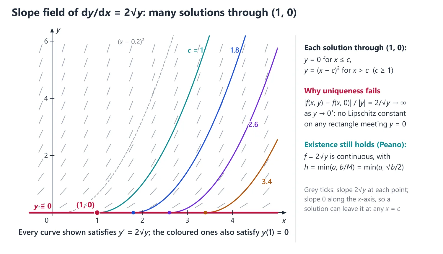
Example 8 (UPSC 2024, 15 marks): State uniqueness theorem for the existence of unique solution of the initial value problem dy/dx = f(x, y), y(x0) = y0 in the rectangular region R : |x − x0| ≤ a, |y − y0| ≤ b. Test the existence and uniqueness of the solution of the initial value problem dy/dx = 2√y, y(1) = 0, in a suitable rectangle R. If more than one solution exist, then find all the solutions.
Statement: as above (Picard's theorem). Here f(x, y) = 2√y, defined for y ≥ 0; take R: |x − 1| ≤ a, 0 ≤ y ≤ b. f is continuous on R with M = 2√b, so a solution exists on |x − 1| ≤ min(a, b/(2√b)) = min(a, √b/2).
Uniqueness is not guaranteed: |f(x, y) − f(x, 0)|/|y − 0| = 2/√y → ∞ as y → 0+, so no Lipschitz constant exists on any rectangle containing points with y = 0.
Solving: y ≡ 0 is a solution. For y > 0, dy/(2√y) = dx gives √y = x − c, that is y = (x − c)2 with x ≥ c.
Joining the two smoothly: for every c ≥ 1, y = 0 for x ≤ c and y = (x − c)2 for x > c is differentiable, satisfies y′ = 2√y and y(1) = 0. (A branch (x − c)2 with x < c is not allowed, since there y′ < 0 while 2√y > 0.)
Answer: solutions exist but are not unique: y ≡ 0 and, for each c ≥ 1, y = 0 (x ≤ c), y = (x − c)2 (x > c); in particular y = (x − 1)2 for x ≥ 1.
17. Geometric, Growth and Formation Problems
Tangent and normal lengths: the tangent at (x, y) is Y − y = p(X − x); it meets the axes at (x − y/p, 0) and (0, y − px). Subtangent = y/p, subnormal = yp, normal length = y√(1 + p2).
Idea: every such problem is "translate the geometric statement into a relation between x, y and p, then solve the ODE". Write the tangent or normal line with running coordinates (X, Y) first, then read off the intercepts.
Growth and decay: dN/dt = kN gives N = N0ekt; doubling time T = (log 2)/k. Newton's law of cooling: dθ/dt = −k(θ − θs) gives θ − θs = (θ0 − θs)e−kt.
Families with n constants: all circles (x − a)2 + (y − b)2 = r2 need 3 differentiations; all conics with axes along the coordinate axes, Ax2 + By2 = 1, need 2.
Example 9 (UPSC 2014, 10 marks): Find the curve for which the part of the tangent cut-off by the axes is bisected at the point of tangency.
The tangent at P(x, y) meets the axes at A(x − y/p, 0) and B(0, y − px). P is the midpoint of AB, so (x − y/p)/2 = x and (y − px)/2 = y.
Either condition gives p = −y/x, that is dy/y + dx/x = 0, so log xy = log c.
Answer: xy = c, a family of rectangular hyperbolas with the axes as asymptotes.
Example 10 (UPSC 2017, 10 marks): Find the differential equation representing all the circles in the x-y plane.
A circle is (x − a)2 + (y − b)2 = r2, with three arbitrary constants. Its radius of curvature is the constant r: (1 + y′2)3/2/y″ = ±r.
Differentiating with respect to x: [3y′y″2(1 + y′2)1/2 − (1 + y′2)3/2y‴]/y″2 = 0.
(Directly: differentiating three times, 1 + y′2 + (y − b)y″ = 0 and 3y′y″ + (y − b)y‴ = 0; eliminating y − b gives the same equation.)
Answer: (1 + y′2)y‴ − 3y′y″2 = 0, a third order equation of degree 1.
Example 11 (UPSC 2025, 10 marks): Form the differential equation of all ellipses whose axes coincide with coordinate axes.
The ellipses are x2/a2 + y2/b2 = 1 (two constants). Differentiating: x/a2 + yy′/b2 = 0, so yy′/x = −b2/a2, a constant.
Differentiating again: [x(y′2 + yy″) − yy′]/x2 = 0.
Answer: xyy″ + xy′2 − yy′ = 0.
Example 12 (UPSC 2017, 8 marks): (ii) If the growth rate of the population of bacteria at any time t is proportional to the amount present at that time and population doubles in one week, then how much bacterias can be expected after 4 weeks?
Let N(t) be the population at time t (weeks): dN/dt = kN, so N = N0ekt.
Doubling in one week: 2N0 = N0ek, so k = log 2 and N = N02t.
Answer: after 4 weeks N = 24N0 = 16N0, sixteen times the initial number.
18. Integrating Factors and Linear Equations: Past Questions
IF as a function of z = x + y: μ(x + y) is an IF of M dx + N dy = 0 if and only if (Nx − My)/(M − N) = φ(x + y); then μ = e∫φ(z) dz. Similarly μ(xy) works if (Nx − My)/(xM − yN) = φ(xy).
Testing a proposed IF μ: μ is an IF exactly when (μM)y = (μN)x, that is μyM − μxN = μ(Nx − My). For μ = xhyk or (x + y)a, compare coefficients to find the exponents.
Variation of parameters for dy/dx + Py = Q: yh = e−∫P dx solves the homogeneous equation; put y = u yh to get u′ = Q/yh.
Example 13 (UPSC 2014, 10 marks): Justify that a differential equation of the form [y + x f(x2 + y2)] dx + [y f(x2 + y2) − x] dy = 0, where f(x2 + y2) is an arbitrary function of (x2 + y2), is not an exact differential equation and 1/(x2 + y2) is an integrating factor for it. Hence solve this differential equation for f(x2 + y2) = (x2 + y2)2.
Write r2 = x2 + y2, f = f(r2). M = y + xf, N = yf − x: My = 1 + 2xyf′, Nx = 2xyf′ − 1, so My − Nx = 2 ≠ 0 and the equation is not exact.
Regroup: (y dx − x dy) + f(r2)(x dx + y dy) = 0. Dividing by r2: −d(tan−1(y/x)) + [f(r2)/r2]·(1/2)d(r2) = 0, each term an exact differential, so 1/(x2 + y2) is an IF.
For f = (x2 + y2)2: −d(tan−1(y/x)) + (1/2)r2 d(r2) = 0, so −tan−1(y/x) + r4/4 = c.
Answer: (x2 + y2)2 = 4 tan−1(y/x) + C.
Example 14 (UPSC 2014, 15 marks): Find the sufficient condition for the differential equation M(x, y) dx + N(x, y) dy = 0 to have an integrating factor as a function of (x + y). What will be the integrating factor in that case? Hence find the integrating factor for the differential equation (x2 + xy) dx + (y2 + xy) dy = 0, and solve it.
Let μ = μ(z), z = x + y, so μx = μy = μ′. Exactness of μM dx + μN dy: μ′M + μMy = μ′N + μNx, that is μ′/μ = (Nx − My)/(M − N).
Sufficient condition: (Nx − My)/(M − N) = φ(x + y), a function of x + y alone; then IF = e∫φ(z) dz.
Here M = x2 + xy, N = y2 + xy: Nx − My = y − x and M − N = (x − y)(x + y), so φ = −1/(x + y) and IF = e−log z = 1/(x + y).
Multiplying: x dx + y dy = 0, which is exact.
Answer: IF = 1/(x + y); the solution is x2 + y2 = c.
Example 15 (UPSC 2015, 12 marks): Find the constant a so that (x + y)a is the Integrating factor of (4x2 + 2xy + 6y)dx + (2x2 + 9y + 3x)dy = 0 and hence solve the differential equation.
M = 4x2 + 2xy + 6y, N = 2x2 + 9y + 3x. For μ = (x + y)a: (μM)y = (μN)x becomes a(M − N) = (x + y)(Nx − My).
M − N = 2x2 + 2xy − 3x − 3y = (x + y)(2x − 3) and Nx − My = (4x + 3) − (2x + 6) = 2x − 3, so a = 1.
The exact equation: (4x3 + 6x2y + 2xy2 + 6xy + 6y2) dx + (2x3 + 2x2y + 3x2 + 12xy + 9y2) dy = 0.
∫M dx = x4 + 2x3y + x2y2 + 3x2y + 6xy2; the term of N free of x is 9y2, giving 3y3.
Answer: a = 1; x4 + 2x3y + x2y2 + 3x2y + 6xy2 + 3y3 = c, that is (x + y)2(x2 + 3y) = c.
Example 16 (UPSC 2018, 12 marks): Find α and β such that xαyβ is an integrating factor of (4y2 + 3xy) dx − (3xy + 2x2) dy = 0 and solve the equation.
With μ = xαyβ: μM = 4xαyβ+2 + 3xα+1yβ+1 and μN = −3xα+1yβ+1 − 2xα+2yβ.
(μM)y = (μN)x: comparing xαyβ+1 terms, 4(β + 2) = −3(α + 1); comparing xα+1yβ terms, 3(β + 1) = −2(α + 2).
That is 3α + 4β = −11 and 2α + 3β = −7, so α = −5, β = 1.
The exact equation (4y3/x5 + 3y2/x4) dx − (3y2/x4 + 2y/x3) dy = 0 has ∫M dx = −y3/x4 − y2/x3, and N has no x-free term.
Answer: α = −5, β = 1; the solution is y3/x4 + y2/x3 = c, that is y2(x + y) = cx4.
Example 17 (UPSC 2020, 10 marks): Solve the following differential equation : x cos(y/x)(y dx + x dy) = y sin(y/x)(x dy − y dx)
Here M = xy cos(y/x) + y2 sin(y/x) and N = x2 cos(y/x) − xy sin(y/x) are homogeneous of degree 2, and Mx + Ny = 2x2y cos(y/x) ≠ 0, so 1/(2x2y cos(y/x)) is an IF (Rule 3).
Quicker by inspection: d(xy cos(y/x)) = (y dx + x dy) cos(y/x) − (y/x) sin(y/x)(x dy − y dx).
So the equation is x·d(xy cos(y/x)) = 0.
Answer: xy cos(y/x) = c.
Example 18 (UPSC 2026, 10 marks): (i) Show that (x + y + 1)−4 is an integrating factor of (2x − y − 1)y dx + (2y − x − 1)x dy = 0. Hence solve it.
M = (2x − y − 1)y, N = (2y − x − 1)x, s = x + y + 1. μ = s−4 is an IF if (μM)y = (μN)x, that is s(My − Nx) = 4(M − N).
My − Nx = (2x − 2y − 1) − (2y − 2x − 1) = 4(x − y), and M − N = x2 − y2 + x − y = (x − y)s. Both sides equal 4(x − y)s, so s−4 is an IF.
Let F = xy/s3: Fx = (ys − 3xy)/s4 = −(2xy − y2 − y)/s4 = −M/s4, and by symmetry Fy = −N/s4. So the exact equation is −dF = 0.
Answer: xy = c(x + y + 1)3.
Example 19 (UPSC 2014, 10 marks): Solve by the method of variation of parameters: dy/dx − 5y = sin x
The homogeneous equation y′ − 5y = 0 has yh = e5x. Put y = u(x)e5x: u′e5x = sin x, so u = ∫e−5x sin x dx.
∫e−5x sin x dx = e−5x(−5 sin x − cos x)/26 + c.
Answer: y = ce5x − (5 sin x + cos x)/26.
Example 20 (UPSC 2022, 10 marks): Show that the general solution of the differential equation dy/dx + Py = Q can be written in the form y = Q/P − e−∫P dx {C + ∫ e∫P dx d(Q/P)}, where P, Q are non-zero functions of x and C, an arbitrary constant.
With I = e∫P dx, dI = PI dx, and the solution of the linear equation is yI = ∫QI dx + C′.
Write QI dx = (Q/P)·PI dx = (Q/P) dI and integrate by parts: ∫(Q/P) dI = (Q/P)I − ∫I d(Q/P).
So yI = (Q/P)I − ∫I d(Q/P) + C′; dividing by I and writing C = −C′: y = Q/P − e−∫P dx{C + ∫e∫P dx d(Q/P)}.
Answer: hence proved (P ≠ 0 is needed to divide by P).
Example 21 (UPSC 2023, 10 marks): Obtain the solution of the initial-value problem dy/dx − 2xy = 2, y(0) = 1 in the form y = ex2[1 + √π erf(x)].
IF = e∫−2x dx = e−x2, so d(ye−x2)/dx = 2e−x2.
Integrating from 0 to x and using y(0) = 1: ye−x2 − 1 = 2∫0x e−t2 dt = √π erf(x), since erf(x) = (2/√π)∫0x e−t2 dt.
Answer: y = ex2[1 + √π erf(x)].
Example 22 (UPSC 2026, 10 marks): If y1 and y2 are two solutions of dy/dx + P(x)y = Q(x), and y2 = y1u, then show that u = 1 + a e−∫(Q/y1) dx, where a is a non-zero constant.
w = y2 − y1 solves the homogeneous equation: w′ + Pw = 0. Also y1′ + Py1 = Q gives P = (Q − y1′)/y1.
With y2 = y1u, w = y1(u − 1). Then y1′(u − 1) + y1u′ + (Q − y1′)(u − 1) = 0, that is y1u′ + Q(u − 1) = 0.
Separating: du/(u − 1) = −(Q/y1) dx, so u − 1 = a e−∫(Q/y1) dx; a ≠ 0 because y2 ≠ y1.
Answer: u = 1 + a e−∫(Q/y1) dx; hence proved.
19. Practice Exercises
Exercise 1 (basic): Find the order and degree of [1 + (dy/dx)2]3/2 = 4 d2y/dx2.
Answer: squaring gives (1 + y′2)3 = 16(y″)2, so the order is 2 and the degree is 2.
Exercise 2 (basic): Show that (x2 + y) dx + (x + ey) dy = 0 is exact and solve it.
Answer: My = 1 = Nx; the solution is x3/3 + xy + ey = c.
Exercise 3 (basic): Form the differential equation whose general solution is y = A cos 2x + B sin 2x.
Answer: two constants, two differentiations: y″ = −4y, that is y″ + 4y = 0 (order 2, degree 1).
Exercise 4 (standard): Solve (x2 + y2) dx − 2xy dy = 0.
Answer: homogeneous; y = vx gives 2v dv/(1 − v2) = dx/x, so x(1 − v2) = C, that is x2 − y2 = Cx.
Exercise 5 (standard): Solve dy/dx + y tan x = sec x.
Answer: IF = e∫tan x dx = sec x; y sec x = tan x + c, that is y = sin x + c cos x.
Exercise 6 (standard): Solve dy/dx + y = xy3.
Answer: Bernoulli with n = 3; z = y−2 gives z′ − 2z = −2x, so z = x + 1/2 + ce2x: 1/y2 = x + 1/2 + ce2x (and y = 0).
Exercise 7 (standard): Solve (xy2 − e1/x3) dx − x2y dy = 0.
Answer: (My − Nx)/N = 4xy/(−x2y) = −4/x, so IF = x−4; the solution is e1/x3/3 − y2/(2x2) = c.
Exercise 8 (UPSC level): Solve (xy3 + y) dx + 2(x2y2 + x + y4) dy = 0.
Answer: (Nx − My)/M = (xy2 + 1)/(y(xy2 + 1)) = 1/y, so IF = y; the solution is 3x2y4 + 6xy2 + 2y6 = c.
Exercise 9 (UPSC level): Solve dy/dx = (x + y + 1)/(2x + 2y + 3).
Answer: the lines are parallel, so put z = x + y: (2z + 3) dz/(3z + 4) = dx; the solution is 6y − 3x + log|3x + 3y + 4| = c.
Exercise 10 (UPSC level): Solve y(2xy + 1) dx + x(1 + 2xy − x3y3) dy = 0.
Answer: Rule 4: Mx − Ny = x4y4, IF = 1/(x4y4); the solution is log y + 1/(x2y2) + 1/(3x3y3) = c.
Exercise 11 (UPSC level): For y′ = x + y, y(0) = 1, compute the Picard iterates y1, y2 starting from y0 = 1 and compare them with the exact solution.
Answer: y1 = 1 + x + x2/2, y2 = 1 + x + x2 + x3/6; the exact solution y = 2ex − x − 1 = 1 + x + x2 + x3/3 + ... agrees with y2 up to x2.
| Type | Standard form | Method |
|---|---|---|
| Separable | f(x) dx = g(y) dy | Integrate both sides |
| Homogeneous | dy/dx = φ(y/x) | y = vx |
| Linear | dy/dx + Py = Q | IF = e∫P dx |
| Bernoulli | dy/dx + Py = Qyn | z = y1−n, then linear |
| Exact | M dx + N dy = 0, My = Nx | ∫M dx + ∫(N-terms free of x) dy = c |
| Non-exact | My ≠ Nx | Find IF by Rules 1-5 or inspection |
Mains points
- Exact-equation and integrating-factor questions are frequent short (10-mark) items; show the test ∂M/∂y = ∂N/∂x before and after multiplying by the IF.
- State which IF rule applies and why (for example, that (My − Nx)/N is a function of x alone); this line earns method marks.
- For Bernoulli equations, write the substitution z = y1−n and the resulting linear equation explicitly before solving.
- In formulation questions the order of the ODE equals the number of independent arbitrary constants; constants such as A + B or AB count as one.
- Common mistake: dividing by a factor such as y or x and losing a solution like y = 0; mention such solutions separately.
Did you know?
- Jacob Bernoulli posed the equation dy/dx + Py = Qyn in 1695, and Leibniz reduced it to a linear equation in 1696.
Orthogonal Trajectories
An orthogonal trajectory of a one-parameter family cuts every member at a right angle. Form the family's ODE by eliminating the parameter, replace dy/dx by −dx/dy (or, in polar form, r dθ/dr by −(1/r) dr/dθ), and solve the new ODE.
1. Understanding Orthogonal Trajectories
Why we need it: in a plane electric field the equipotential lines and the lines of force always cross at right angles, and in a steady flow the streamlines cross the lines of equal potential at right angles. Given one of the two families, the physics asks for the other. More generally, given a family of curves, we want the curves that meet every member at a prescribed angle.
In words: a one-parameter family is a collection of curves f(x, y, c) = 0, one curve for each value of the parameter c. Two curves cut at angle θ at a common point if their tangent lines there make the angle θ. An orthogonal trajectory is a curve that is perpendicular to every member it meets, at every meeting point.
Usually exactly one member and one trajectory pass through each point of the region, so the trajectories themselves form a new one-parameter family with a new constant k.
First example, slowly: find the orthogonal trajectories of the lines through the origin, y = cx. The picture to expect: circles centred at the origin cut every radius at a right angle.
(1) The family's slope: dy/dx = c, and c = y/x, so at the point (x, y) the member through it has slope y/x. (2) A trajectory through the same point must have slope mT with mT·(y/x) = −1, so mT = −x/y.
(3) Solve dy/dx = −x/y: y dy = −x dx, so x2 + y2 = k. (4) Check: at (x, y) the radius has direction (x, y) and the circle's tangent has direction (−y, x); their dot product is −xy + yx = 0, so they are perpendicular, as expected.
Non-example: the lines y = x + c meet the circles x2 + y2 = k, but the product of slopes is 1·(−x/y) = −x/y, which equals −1 only at points of the line y = x. They are perpendicular at some meeting points only, so they are not orthogonal trajectories: the right angle is required at every intersection.
Building up: the family's ODE F(x, y, p) = 0 gives at each point the slope p of the member there. A trajectory's slope pT satisfies p·pT = −1, that is p = −1/pT. Substituting, F(x, y, −1/pT) = 0 is the ODE of the trajectories, and its general solution brings the new constant k that labels them.
Where it is used: electrostatics (field lines and equipotentials), ideal fluid flow (streamlines ψ = c and equipotentials φ = c), heat flow (flow lines and isotherms), and the harmonic conjugate of Complex Analysis.
2. Definition
A curve that cuts every member of a given one-parameter family f(x, y, c) = 0 at a right angle is an orthogonal trajectory of the family.
Physical uses: lines of force and equipotential curves in electrostatics, streamlines and equipotential lines in fluid flow, heat-flow lines and isotherms.
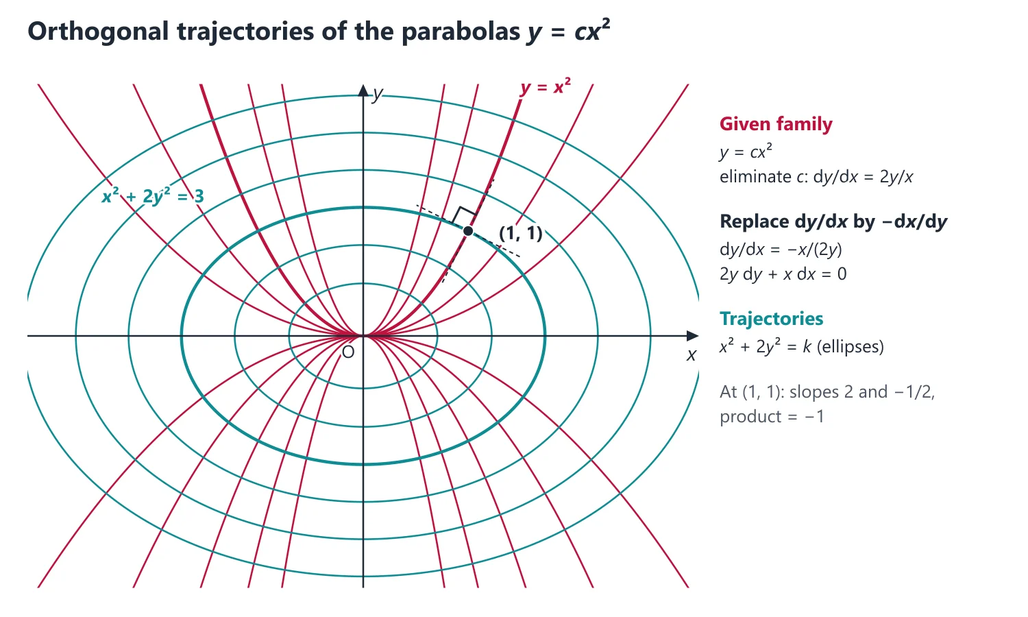
Idea: see the figure above: the parabolas y2 = 4ax and the ellipses 2x2 + y2 = k (Example 1) cross at right angles at every point where they meet. The trajectories form another one-parameter family, so the answer always contains a new arbitrary constant.
In a plane electrostatic field the equipotentials φ = c and the lines of force are orthogonal families; in steady plane flow of an ideal fluid the same holds for equipotentials and streamlines ψ = c. Finding one family from the other is exactly the problem of this topic.
3. Understanding the Differential Equation of a Family
Why we need it: the perpendicularity condition must be applied point by point, but the family is described with a parameter c that changes from member to member. At a given point we must know the slope of the member through that point, expressed through the point alone.
In words: the differential equation of the family is the relation F(x, y, p) = 0 obtained by eliminating c between f(x, y, c) = 0 and its derivative fx + fyp = 0. It assigns to each point (x, y) the slope of the member that passes through it, so it is a "slope field" with no parameter left.
First example, slowly: the parabolas y = cx2. (1) Differentiate: p = 2cx. (2) From the family, c = y/x2. (3) Substitute: p = 2y/x; check on the member y = 3x2 at (1, 3): its slope is 6, and 2·3/1 = 6.
(4) For the trajectories replace p by −1/p: −1/p = 2y/x, so dy/dx = −x/(2y) and 2y dy = −x dx. (5) Integrate: x2 + 2y2 = k, a family of ellipses. Notice that the parameter c disappeared in step (3), before the slope was inverted.
Non-example: inverting before eliminating: from p = 2cx write −1/p = 2cx, so dy/dx = −1/(2cx) and y = −(1/(2c)) log x + k. This still contains c; it gives a different curve for each parabola, and these curves do not cross all the parabolas at right angles. It is not the trajectory family.
Building up: if the family is written as u(x, y) = c, implicit differentiation gives the member's slope −ux/uy directly, with c already gone. The trajectories then solve dy/dx = uy/ux: they run along the gradient ∇u, which is perpendicular to the level curves of u. For y = cx2, u = y/x2 gives dy/dx = (1/x2)/(−2y/x3) = −x/(2y), as above.
Where it is used: it is Step 1 of every Cartesian and polar trajectory problem, of every self-orthogonality proof, and of the formation questions of the first topic.
4. Method in Cartesian Coordinates
Step 1: Differentiate f(x, y, c) = 0 and eliminate c to get the family's ODE F(x, y, dy/dx) = 0.
Why eliminate c: the slope of the family at a point must be expressed through the point alone, since the trajectory meets different members at different points. The ODE F(x, y, y′) = 0 gives, at each point, the slope of the member through that point.
Step 2: Replace dy/dx by −dx/dy (perpendicular slopes satisfy m1m2 = −1).
Why it works: at a common point, if the member has slope p and the trajectory has slope pT, then p pT = −1, so p = −1/pT. Writing −dx/dy rather than −1/(dy/dx) also covers points where the trajectory is vertical.
Step 3: Solve the new ODE; its general solution is the family of orthogonal trajectories.
Example 1: Find the orthogonal trajectories of the parabolas y2 = 4ax.
Differentiating, 2yy′ = 4a = y2/x, so the family's ODE is y = 2x dy/dx.
Replacing dy/dx by −dx/dy: y dy = −2x dx, so y2/2 + x2 = c, that is 2x2 + y2 = k, a family of ellipses.
5. Understanding the Polar Angle ψ
Why we need it: cardioids r = a(1 + cos θ), lemniscates and spirals are awkward in x and y. In polar coordinates the slope dy/dx is messy, but the angle between the radius vector and the tangent has a very simple formula, and right angles between curves can be tested with it.
In words: at a point P of r = r(θ), ψ is the angle from the radius vector OP to the tangent at P, measured in the sense of increasing θ, and tan ψ = r dθ/dr. Two curves through P have tangent directions θ + ψ1 and θ + ψ2, so the angle between them is ψ1 − ψ2; they are orthogonal exactly when tan ψ1 tan ψ2 = −1.
First example, slowly: two quick values of ψ, then a trajectory. (1) For the circle r = a, dr/dθ = 0, so tan ψ is infinite and ψ = 90°: the radius is perpendicular to the tangent, as it should be. (2) For the spiral r = eθ, dr/dθ = r, so tan ψ = 1 and ψ = 45° at every point.
(3) Trajectories of the circles r = a: take logarithms, log r = log a, and differentiate in θ: (1/r) dr/dθ = 0. (4) Replace (1/r) dr/dθ by −r dθ/dr: −r dθ/dr = 0, so dθ/dr = 0 and θ = k. (5) The trajectories are the rays from the pole, the same answer as in the first lesson with the roles of the two families exchanged.
Non-example: replacing dr/dθ by −dθ/dr (dropping the factor r2) is not the orthogonality rule. The correct rule comes from tan ψT = −1/tan ψ, that is r dθ/dr → −(1/r) dr/dθ, which has r on both sides; the wrong replacement changes the angle condition and gives curves that are not perpendicular to the family.
Building up: the position vector is r er, and its θ-derivative, the tangent vector, is (dr/dθ)er + r eθ (derived in the section on the polar formula below). Its components along the radius and across it are dr/dθ and r, so tan ψ = r/(dr/dθ). Taking logarithms of the family before differentiating, log r = log a + log g(θ), gives (1/r) dr/dθ = g′(θ)/g(θ) with the constant a already removed.
Where it is used: trajectories of cardioids, of rn = an cos nθ and of circles through the pole are standard 10–12 mark questions; the same angle ψ appears in polar arc length and curvature in Calculus and in central orbits in Dynamics.
6. Method in Polar Coordinates
The angle ψ between the radius vector and the tangent satisfies tan ψ = r dθ/dr.
For orthogonal curves tan ψ1 tan ψ2 = −1, so replace r dθ/dr by −(1/r) dr/dθ, equivalently replace dr/dθ by −r2 dθ/dr.
Idea: ψ is the angle from the radius vector to the tangent (derived below). The angle between two curves at a common point is ψ1 − ψ2, and this is 90° exactly when 1 + tan ψ1 tan ψ2 = 0.
When to use polar form: when the family contains r and θ naturally (cardioids, rn = an cos nθ, spirals), or when x2 + y2 and y/x appear in a Cartesian equation. Taking logarithms before differentiating usually removes the constant at once.
Example 2: Find the orthogonal trajectories of the cardioids r = a(1 + cos θ).
Taking logarithms and differentiating: (1/r) dr/dθ = −sin θ/(1 + cos θ) = −tan(θ/2).
Replacing (1/r) dr/dθ by −r dθ/dr: r dθ/dr = tan(θ/2), so dr/r = cot(θ/2) dθ.
Integrating, log r = 2 log sin(θ/2) + log c, so r = c sin2(θ/2) = b(1 − cos θ) with b = c/2: another family of cardioids.
7. Understanding Oblique Trajectories and Self-Orthogonal Families
Why we need it: sometimes the required angle is not 90° (a spiral that cuts every radius at 45°), and sometimes a family turns out to be its own orthogonal family (confocal conics), which examiners like to ask as a "show that" question.
In words: an oblique trajectory at angle α cuts every member at the constant angle α. If the trajectory's tangent makes the angle φ with the x-axis, the member's tangent makes φ − α (or φ + α for the other sense), so the member's slope is tan(φ − α) = (p − tan α)/(1 + p tan α), where p = tan φ is the trajectory's slope.
A family is self-orthogonal when its ODE is unchanged by p → −1/p. Then the trajectories satisfy the same ODE as the family, so every trajectory is itself a member: through each point pass two members, and they cross at right angles.
First example, slowly: find the curves cutting the parallel lines y = x + c at 45°. (1) The family's ODE is p = 1. (2) Replace p by (p − 1)/(1 + p): (p − 1)/(1 + p) = 1 gives p − 1 = 1 + p, that is −1 = 1, so no finite slope works; the trajectory must be vertical, x = k.
(3) The other sense of rotation uses (p + 1)/(1 − p) = 1, which gives p = 0: the horizontal lines y = k. (4) Check: a line of slope 1 makes 45° with both axes. Notice that the two senses give two different families, so state both unless the sense is specified.
Self-orthogonality test for a quadratic in p: if the ODE is Ap2 + Bp + C = 0, replacing p by −1/p and multiplying by p2 gives Cp2 − Bp + A = 0. This is the same equation (up to the factor −1) exactly when C = −A, that is when the product of the two roots C/A is −1: the two members through a point have perpendicular slopes.
Non-example: the circles x2 + y2 = 2cx have the ODE 2xyp = y2 − x2, which is linear in p. Replacing p by −1/p gives (y2 − x2)p + 2xy = 0, a different equation, so the family is not self-orthogonal; its trajectories are the different circles x2 + y2 = 2ky (Example 4). Only one member passes through each point, so there is no second member to be perpendicular to.
Building up: for the confocal conics x2/(a2 + λ) + y2/(b2 + λ) = 1, the ODE (x + yp)(x − y/p) = a2 − b2 (Example 8) multiplies out to xyp2 + (x2 − y2 − a2 + b2)p − xy = 0. The coefficients of p2 and p0 are xy and −xy, so the test above shows at once that the family is self-orthogonal.
Where it is used: equiangular spirals (curves at a constant angle to all radii), "show that the family is self-orthogonal" for confocal conics and for the parabolas y2 = 4a(x + a), and the polar oblique rule tan(ψ − α).
8. Self-Orthogonal Families and Oblique Trajectories
A family is self-orthogonal if its ODE is unchanged when dy/dx is replaced by −dx/dy.
Idea: through each point of the plane pass two members of a self-orthogonal family, and they cut at right angles (for confocal conics, one ellipse and one hyperbola). The family's ODE is typically quadratic in p with the product of its roots equal to −1.
Standard examples: the confocal conics x2/(a2 + λ) + y2/(b2 + λ) = 1 and the confocal parabolas y2 = 4a(x + a).
Oblique trajectories cut each curve at a constant angle α: replace dy/dx = p by (p − tan α)/(1 + p tan α).
Why it works: let the trajectory make angle φ with the x-axis, so p = tan φ, and let it be turned through α from the member, whose slope is then tan(φ − α) = (p − tan α)/(1 + p tan α). The other sense of rotation uses (p + tan α)/(1 − p tan α). As α → 90° both tend to −1/p, the orthogonal rule.
Polar oblique trajectories: replace tan ψ = r dθ/dr by tan(ψ − α) = (r dθ/dr − tan α)/(1 + tan α · r dθ/dr).
Example 3: Show that the family y2 = 4a(x + a) is self-orthogonal.
Differentiating, yp = 2a with p = y′, so y2 = 2yp(x + yp/2), that is y = 2xp + yp2.
Replacing p by −1/p gives y = −2x/p + y/p2; multiplying by p2, yp2 = −2xp + y, which is the same equation, so the family is self-orthogonal.
Example 4: For the circles x2 + y2 = 2cx, eliminating c gives dy/dx = (y2 − x2)/(2xy).
The trajectories satisfy dy/dx = 2xy/(x2 − y2), a homogeneous equation whose solution is x2 + y2 = 2ky: circles touching the x-axis at the origin.
9. Derivation: The Polar Formula tan ψ = r dθ/dr
A point of the curve r = r(θ) is r(cos θ, sin θ). Let er = (cos θ, sin θ) and eθ = (−sin θ, cos θ) be the radial and transverse unit vectors.
Differentiating with respect to θ, the tangent vector is (dr/dθ)er + r eθ.
Its components along er and eθ are dr/dθ and r, so the angle ψ from the radius vector to the tangent satisfies tan ψ = r/(dr/dθ) = r dθ/dr.
For orthogonal curves tan ψT = −1/tan ψ, so in the family's equation r dθ/dr is replaced by −1/(r dθ/dr) = −(1/r) dr/dθ, the rule stated above.
10. Derivation: Two Short Cuts
Family solved for the constant: if the family is u(x, y) = c, its slope is −ux/uy, so the trajectories satisfy dy/dx = uy/ux: they run along the gradient ∇u. For y2/x = 4a this gives dy/dx = (2y/x)/(−y2/x2) = −2x/y, hence 2x2 + y2 = k, as in Example 1.
Harmonic families: if f(z) = u + iv is analytic, the Cauchy-Riemann equations ux = vy, uy = −vx give ∇u · ∇v = uxvx + uyvy = 0. So the curves u = c and v = c are orthogonal wherever f′(z) ≠ 0.
For example z2 = (x2 − y2) + 2ixy shows that the hyperbolas x2 − y2 = c and xy = k are orthogonal, and ez shows that ex cos y = c and ex sin y = k are orthogonal.
11. Choosing the Method
If the family is easily written as u(x, y) = c → dy/dx = uy/ux directly.
If the family is given in polar form, or contains x2 + y2 and y/x → polar method: take logarithms, differentiate with respect to θ, replace (1/r) dr/dθ by −r dθ/dr.
If u is the real or imaginary part of a familiar analytic function → the trajectories are the level curves of its harmonic conjugate.
If the curves must cut at a constant angle α ≠ 90° → oblique rule; if self-orthogonality is to be shown → derive the ODE, replace p by −1/p and show it is unchanged.
Then solve the trajectory ODE with the first order methods: it is often separable, homogeneous (Example 4) or linear.
12. Common Mistakes
Replacing p before eliminating the parameter; the resulting equation still contains the old constant and its solution is not the trajectory family.
Replacing dy/dx by dx/dy or by −dy/dx instead of −dx/dy.
In polar form, replacing dr/dθ by −dθ/dr instead of −r2 dθ/dr.
Writing the answer with the same letter as the constant of the given family, which suggests that the trajectories are the given curves; use a new constant, and for a self-orthogonal family say so explicitly.
Dividing by x or y and missing trajectories that lie along an axis (for the circles x2 + y2 = a2 every line through the origin, including the y-axis, is a trajectory).
13. Connections
Link: harmonic conjugates and the Cauchy-Riemann equations (Complex Analysis) give orthogonal families at once; in Fluid Dynamics the velocity potential φ and stream function ψ of a plane irrotational flow are such a pair.
Link: the gradient of u is normal to its level curves (Vector Analysis), which is why the orthogonal trajectories of u = c are the lines of steepest ascent of u.
14. Worked Examples
Example 5: Find the orthogonal trajectories of the family of cubical parabolas y = ax3.
Differentiating, dy/dx = 3ax2 = 3y/x, which is the family's ODE.
Replacing dy/dx by −dx/dy: −dx/dy = 3y/x, so x dx + 3y dy = 0 and x2 + 3y2 = c: a family of similar ellipses.
Example 6: Show that the orthogonal trajectories of rn = an cos nθ are the curves rn = bn sin nθ.
Taking logarithms, n log r = n log a + log cos nθ; differentiating with respect to θ, (1/r) dr/dθ = −tan nθ.
Replacing (1/r) dr/dθ by −r dθ/dr: r dθ/dr = tan nθ, so dr/r = cot nθ dθ.
Integrating, log r = (1/n) log sin nθ + log b, so rn = bn sin nθ (for n = 2 these are two orthogonal families of lemniscates).
Example 7: Find the curves that cut every line through the origin at the constant angle 45°.
The family y = cx has ODE p = y/x; for oblique trajectories replace p by (p − tan 45°)/(1 + p tan 45°) = (p − 1)/(1 + p).
(p − 1)/(1 + p) = y/x gives dy/dx = (x + y)/(x − y), a homogeneous equation; in polar form it reads r dθ/dr = 1.
Hence log r = θ + c, that is r = Ceθ (equivalently log √(x2 + y2) = tan−1(y/x) + c): equiangular spirals.
15. Confocal Conics
For x2/(a2 + λ) + y2/(b2 + λ) = 1, the ellipses (λ > −b2) and hyperbolas (−a2 < λ < −b2) have the same foci (±√(a2 − b2), 0); through each point not on the axes pass one ellipse and one hyperbola of the family, and they cut at right angles.
Idea: as λ varies the curve changes from an ellipse to a hyperbola as λ passes −b2, while the foci stay fixed because (a2 + λ) − (b2 + λ) = a2 − b2 does not depend on λ. The orthogonality is the reflection property: the tangent to the ellipse bisects the external angle between the focal radii, the tangent to the hyperbola bisects the internal angle, and these bisectors are perpendicular.
Example 8 (UPSC 2021, 10 marks): (i) Find the orthogonal trajectories of the family of confocal conics x2/(a2 + λ) + y2/(b2 + λ) = 1; a > b > 0 are constants and λ is a parameter. Show that the given family of curves is self orthogonal.
Let A = a2 + λ, B = b2 + λ, so A − B = a2 − b2. Differentiating: x/A + yp/B = 0, so B = −ypA/x.
Then A(1 + yp/x) = a2 − b2, giving A = (a2 − b2)x/(x + yp) and B = −(a2 − b2)yp/(x + yp).
Substituting in x2/A + y2/B = 1: (x + yp)(x − y/p) = a2 − b2, the ODE of the family.
Replace p by −1/p: (x − y/p)(x + yp) = a2 − b2, the same equation. So the orthogonal trajectories are the family itself.
Answer: the orthogonal trajectories are x2/(a2 + μ) + y2/(b2 + μ) = 1; the family is self-orthogonal.
16. Practice Exercises
Exercise 1 (basic): Find the orthogonal trajectories of the rectangular hyperbolas xy = c.
Answer: family ODE p = −y/x; trajectories dy/dx = x/y, that is x2 − y2 = k.
Exercise 2 (basic): Find the orthogonal trajectories of y = cex.
Answer: family ODE p = y; trajectories −dx/dy = y, so y2 + 2x = k (parabolas).
Exercise 3 (basic): Show that the circles x2 + y2 = k are the orthogonal trajectories of the lines y = cx, by checking that the product of the slopes at every common point is −1.
Answer: the line has slope y/x and the circle has slope −x/y at (x, y); the product is −1 (on the axes one slope is 0 and the other infinite).
Exercise 4 (standard): Find the orthogonal trajectories of the semicubical parabolas y2 = cx3.
Answer: family ODE p = 3y/(2x); trajectories 2x dx + 3y dy = 0, that is 2x2 + 3y2 = k.
Exercise 5 (standard): Find the orthogonal trajectories of the circles r = 2a cos θ through the pole.
Answer: (1/r) dr/dθ = −tan θ; replacing gives dr/r = cot θ dθ, so r = b sin θ: circles touching the initial line at the pole.
Exercise 6 (standard): Find the orthogonal trajectories of the confocal parabolas r = a/(1 + cos θ).
Answer: (1/r) dr/dθ = tan(θ/2); replacing gives dr/r = −cot(θ/2) dθ, so r = b/(1 − cos θ): the coaxial parabolas opening the other way.
Exercise 7 (standard): Using u = ex cos y, find the orthogonal trajectories of ex cos y = c.
Answer: dy/dx = uy/ux = −tan y gives cot y dy = −dx, so ex sin y = k (the harmonic conjugate of u).
Exercise 8 (UPSC level): Find the curves that cut every circle x2 + y2 = a2 (a the parameter) at an angle of 45°.
Answer: replacing p in p = −x/y by (p ∓ 1)/(1 ± p) gives dy/dx = (y − x)/(y + x) or (x + y)/(x − y); in polar form r = Ce−θ and r = Ceθ, equiangular spirals.
Exercise 9 (UPSC level): Show that the family of parabolas x2 = 4a(y + a) is self-orthogonal.
Answer: a = x/(2p) gives the ODE xp2 − 2yp − x = 0; the coefficients of p2 and p0 are x and −x, so p → −1/p leaves it unchanged.
Exercise 10 (UPSC level): Find the orthogonal trajectories of rn sin nθ = an.
Answer: (1/r) dr/dθ = −cot nθ; replacing gives dr/r = tan nθ dθ, so rn cos nθ = bn (the real and imaginary parts of zn).
| Setting | Replace | By |
|---|---|---|
| Cartesian, orthogonal | dy/dx | −dx/dy |
| Polar, orthogonal | r dθ/dr | −(1/r) dr/dθ |
| Polar, orthogonal (equivalent form) | dr/dθ | −r2 dθ/dr |
| Cartesian, oblique at angle α | p = dy/dx | (p − tan α)/(1 + p tan α) |
Mains points
- A standard 10-12 mark question: find the orthogonal trajectories of a given family, often in polar form (cardioids, rn = an cos nθ, circles through the pole).
- Eliminate the parameter completely before replacing the slope; replacing first and eliminating later gives a wrong answer.
- In polar problems take logarithms before differentiating; this removes the constant a in one step.
- Name the resulting family (ellipses, circles, cardioids) in the final line; a sketch of both families earns presentation credit.
- To prove a family is self-orthogonal, show its ODE is invariant under p → −1/p; this is a common short question.
Did you know?
- The family rn = an cos nθ has orthogonal trajectories rn = bn sin nθ; n = 1 gives circles through the pole, n = 2 lemniscates and n = 1/2 cardioids.
First Order Higher Degree Equations, Clairaut's Equation and Singular Solutions
Equations F(x, y, p) = 0 with p = dy/dx of degree higher than one are solved by treating them as solvable for p, y or x. Clairaut's equation y = px + f(p) has general solution y = cx + f(c) and a singular solution, the envelope of these lines, found from x + f′(p) = 0.
1. Understanding Equations of Higher Degree in p
Why we need it: geometric conditions often produce equations in which the slope p = dy/dx appears squared or cubed, for instance "the tangent is at unit distance from the origin". Such an equation cannot be written as dy/dx = f(x, y), so the first order methods of the previous topics do not apply directly.
In words: a first order equation of degree n is F(x, y, p) = 0 with F a polynomial of degree n in p. At a point (x, y) it is an algebraic equation for p, with up to n real roots, so up to n solution curves pass through the point with different slopes. There are three standard routes: solve the equation for p (factorise), solve it for y, or solve it for x.
First example, slowly: solve p2 − (x + y)p + xy = 0. (1) Treat it as a quadratic in p and factorise: (p − x)(p − y) = 0. (2) The factor p = x gives y = x2/2 + c, that is 2y − x2 − c = 0 (renaming the constant).
(3) The factor p = y gives y = cex, that is y − cex = 0. (4) The general solution is the union of both families, written with one constant: (2y − x2 − c)(y − cex) = 0. (5) Notice what it means: through the point (1, 1) pass one parabola (slope 1) and one exponential (slope 1), and through (2, 1) slopes 2 and 1.
At (1, 1) the two slopes coincide; such points, where two roots p become equal, are exactly where the discriminant of the quadratic, (x + y)2 − 4xy = (x − y)2, vanishes. Keep this in mind for the lessons on singular solutions below.
Non-example: xp2 − 2yp + 4x = 0 (Example 6) does not factorise into factors linear in p with simple coefficients, so "solvable for p" leads to square roots √(y2 − 4x2) that are hard to integrate. It is solvable for y instead: y = xp/2 + 2x/p. Recognising which variable to isolate is the main skill.
Building up: when y = f(x, p), differentiating in x gives p = fx + fp dp/dx, a first order equation in x and p only, because y has disappeared. Solve it as φ(x, p, c) = 0 and eliminate p with y = f(x, p), or keep p as a parameter. When x = f(y, p), differentiate in y and use dx/dy = 1/p in the same way.
Where it is used: the three routes cover every higher degree question in the syllabus; "solvable for y" contains Clairaut's and Lagrange's equations as special cases.
2. Equations of First Order and Higher Degree
With p = dy/dx the general form is pn + P1pn−1 + ... + Pn = 0, where the Pi are functions of x and y.
Idea: an equation of degree n in p prescribes up to n slopes at each point, so up to n integral curves pass through a point instead of one. Where two of these slopes coincide, curves can touch, and that is where singular solutions live.
Solvable for p: factor as (p − f1)(p − f2)...(p − fn) = 0, solve each factor to get φi(x, y, c) = 0, and write the solution as φ1φ2...φn = 0 with a single constant c.
Why one constant: each factor gives a one-parameter family, and the general solution is the union of these families; using c1, c2, ... separately adds nothing, because each factor is satisfied on its own curves. The convention is to write the product with a single c.
Solvable for y: y = f(x, p); differentiate with respect to x to get p = F(x, p, dp/dx), solve this for p, and eliminate p.
Why it works: differentiating y = f(x, p) removes y and leaves a first order equation in x and p only. Its solution φ(x, p, c) = 0, together with y = f(x, p), is the general solution; when p cannot be eliminated neatly, the answer may be left in parametric form with p as parameter.
Solvable for x: x = f(y, p); differentiate with respect to y using dx/dy = 1/p, solve, and eliminate p.
Example 1: Solve p2 − 5p + 6 = 0.
(p − 2)(p − 3) = 0 gives y = 2x + c and y = 3x + c, so the solution is (y − 2x − c)(y − 3x − c) = 0.
3. Understanding Clairaut's Equation
Why we need it: many geometric questions are about families of straight lines (tangent lines of a curve, lines whose intercepts satisfy a condition). Their differential equations have a special shape, y = px + f(p), and for this shape the general solution can be written down without any integration, while a second, curved solution appears that is not in the family.
In words: Clairaut's equation is y = px + f(p): y equals x times the slope plus a function of the slope alone. A straight line y = cx + f(c) has constant slope p = c, so it satisfies the equation; these lines form the general solution. The curve that touches all these lines (their envelope) also satisfies the equation, because at each of its points it has the same x, y and p as one of the lines; it is the singular solution.
First example, slowly: solve y = px − p2. (1) It is of Clairaut's form with f(p) = −p2. (2) General solution: write c for p, y = cx − c2, a family of lines.
(3) Singular solution: the other factor after differentiating is x + f′(p) = x − 2p = 0, so p = x/2. (4) Substitute in the equation: y = (x/2)x − x2/4 = x2/4, that is x2 = 4y, a parabola.
(5) Check the picture: the tangent to x2 = 4y at (2t, t2) is y = tx − t2, which is the member c = t. So the general solution is the set of all tangent lines of the parabola, and the parabola itself is the singular solution; it is not a line, so no value of c produces it.
Non-example: y = 2px + p2 (Example 4) looks similar, but the coefficient of x is 2p, not p. Writing p = c gives y = 2cx + c2, whose slope is 2c, not c, so it is not a solution. This is Lagrange's equation and must be differentiated and solved as a linear equation in x(p).
Building up: differentiating y = px + f(p) gives p = p + [x + f′(p)] dp/dx, so [x + f′(p)] dp/dx = 0 (derived in this section). Either dp/dx = 0, which gives the lines, or x + f′(p) = 0, which together with the equation gives the envelope in parametric form x = −f′(p), y = f(p) − pf′(p).
Many equations become Clairaut's only after a change of variables u(x, y), v(x, y): the new slope is P = dv/du = (vx + vyp)/(ux + uyp), and the aim is to make the equation read v = Pu + f(P). The table of standard substitutions later in this topic lists the usual choices.
Where it is used: Clairaut questions (direct or after X = x2, Y = y2) appear almost every year; the envelope idea links to envelopes of planes in Analytic Geometry and to the complete and singular integrals of Clairaut's PDE z = px + qy + f(p, q).
4. Clairaut's Equation
Form: y = px + f(p).
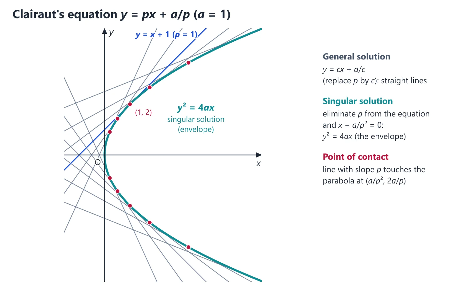
Idea: the general solution y = cx + f(c) is a family of straight lines, and the singular solution is the curve they all touch (see the figure above: the lines y = cx + a/c and their envelope, the parabola y2 = 4ax of Example 2).
Differentiating with respect to x: p = p + x dp/dx + f′(p) dp/dx, so (x + f′(p)) dp/dx = 0.
dp/dx = 0 gives p = c and the general solution y = cx + f(c), obtained simply by writing c for p.
x + f′(p) = 0 together with y = px + f(p), on eliminating p, gives the singular solution, which is the envelope of the lines y = cx + f(c).
Why it is the envelope: for φ(x, y, c) = y − cx − f(c), the c-discriminant equations are φ = 0 and ∂φ/∂c = −x − f′(c) = 0, which are the same as y = px + f(p) and x + f′(p) = 0 with p = c. For Clairaut's equation the p- and c-discriminants coincide.
Example 2: Solve y = px + a/p.
General solution: y = cx + a/c.
From x − a/p2 = 0, p = √(a/x); then y = x√(a/x) + a√(x/a) = 2√(ax), so the singular solution is y2 = 4ax.
Reduction to Clairaut's form: (px − y)(py + x) = a2p becomes Y = PX − a2P/(P + 1) by X = x2, Y = y2, P = dY/dX = yp/x; other equations reduce by substitutions such as X = ex, Y = ey.
Lagrange's equation: y = xφ(p) + ψ(p) with φ(p) ≠ p; differentiating with respect to x gives an equation linear in x when p is taken as the independent variable.
5. Understanding Envelopes and Singular Solutions
Why we need it: a general solution with one constant usually gives all solutions, but not always. A curve that touches every member of the family is itself a solution that no value of c produces, and an exam answer that misses it is incomplete. We need a way to find such curves and to decide whether they really are solutions.
In words: the envelope of a family φ(x, y, c) = 0 is a curve that, at each of its points, touches some member of the family. It is found by eliminating c between φ = 0 and ∂φ/∂c = 0: the second equation says that two members with neighbouring values of c pass through the point. A singular solution is a solution of the ODE not contained in the general solution; geometrically it is the envelope.
First example, slowly: the circles (x − c)2 + y2 = 1 of radius 1 with centres on the x-axis. (1) Their ODE: differentiating, (x − c) + yp = 0, so x − c = −yp; substituting, y2p2 + y2 = 1, that is y2(1 + p2) = 1.
(2) Envelope: ∂φ/∂c = −2(x − c) = 0 gives c = x, and then y2 = 1, so y = 1 and y = −1. (3) Test in the ODE: on y = 1, p = 0 and y2(1 + p2) = 1, true; the same for y = −1.
(4) Is y = 1 a member? No member is a straight line, so no value of c gives it. (5) Conclusion: y = ±1 are singular solutions, the two lines that every circle touches at its top and bottom points. Notice that through (0, 1) pass two solutions with slope 0: the line y = 1 and the circle with c = 0, so uniqueness fails on the envelope.
Non-example: the x-axis y = 0 passes through the centre of every circle and crosses each one at right angles; it touches none of them and on it the ODE reads 0 = 1, so it is not a solution. Similarly, the general solution y = sin(x + c) of p2 + y2 = 1 contains y = 0 for no c either, but y = 0 fails the ODE (p = 0 gives 0 = 1), so "not in the family" alone does not make a curve a singular solution: it must also satisfy the equation.
Building up: why the envelope satisfies the ODE is proved in the derivation section below: along the envelope φc = 0, so its slope satisfies the same relation φx + φyy′ = 0 as the member it touches. So it shares x, y and p with that member at every point, and F(x, y, p) = 0 holds along it.
Where it is used: every Clairaut question, every "find the singular solution" question, and the envelope problems of Analytic Geometry use the same elimination of c.
6. Understanding the p- and c-Discriminants
Why we need it: eliminating c (or p) produces a curve, but that curve can contain pieces that are not solutions at all: places where members touch each other, cross themselves or have cusps. To answer correctly we must sort the factors of the discriminants and keep only the true envelope.
In words: the p-discriminant is obtained by eliminating p from F(x, y, p) = 0 and ∂F/∂p = 0; it is the locus where two of the slopes at a point coincide. The c-discriminant is obtained by eliminating c from φ(x, y, c) = 0 and ∂φ/∂c = 0; it is the locus where two neighbouring members meet. The envelope E occurs once in both; a tac-locus T (two non-neighbouring members touching) occurs squared in the p-discriminant only; a nodal locus N occurs squared in the c-discriminant only; a cusp locus C occurs once in the p- and cubed in the c-discriminant.
First example, slowly: continue with y2(1 + p2) = 1, that is y2p2 + (y2 − 1) = 0. (1) As a quadratic Ap2 + Bp + C with A = y2, B = 0, C = y2 − 1, the p-discriminant is B2 − 4AC = −4y2(y2 − 1) = 0, giving the factors y2 (squared) and y2 − 1 (once).
(2) The c-discriminant (previous lesson) is y2 − 1 = 0 only. (3) Sort: y2 − 1 occurs once in both, so y = ±1 is the envelope; y = 0 occurs squared in the p-discriminant and not in the c-discriminant, so it is a tac-locus.
(4) Check the geometry: the circles with centres c and c + 2 touch each other at (c + 1, 0), on the x-axis, and they are not neighbours. (5) Final answer: singular solutions y = ±1 only; y = 0 is a tac-locus and does not satisfy the ODE.
Non-example: for (x − c)2 = y2(3 − y) (Example 12) the c-discriminant contains y2, but y = 0 is a nodal locus (each member crosses itself there) and does not satisfy the equation. A factor of a discriminant is only a candidate; the multiplicity pattern and substitution in the ODE decide.
Building up: on the p-discriminant ∂F/∂p = 0, so the implicit function theorem cannot solve F = 0 smoothly for p there; this is where several solution curves can share a slope, either because they touch an envelope (E) or because two separate members touch (T). The multiplicities in the table of discriminant factors come from local expansions of F and φ near each kind of locus; for the exam it is enough to quote them and always verify by substitution.
Where it is used: 10–15 mark questions of the form "find the general and singular solutions and interpret them geometrically"; the same ∂/∂c = 0 elimination gives envelopes of planes and spheres in Analytic Geometry.
7. Singular Solution
A singular solution satisfies the ODE but is not obtained from the general solution for any value of c; geometrically it is the envelope of the family of integral curves.
Idea: at each point of the envelope it touches some member of the family, so it has the same x, y and p as that member and therefore satisfies the ODE; but it is not itself a member. Through such a point two solution curves pass with the same slope, so uniqueness fails there.
p-discriminant: eliminate p between F(x, y, p) = 0 and ∂F/∂p = 0.
Idea: F = 0 and ∂F/∂p = 0 together mean that p is a repeated root of F(x, y, p) = 0: the p-discriminant is the locus of points where two of the n slopes coincide. For a quadratic Ap2 + Bp + C = 0 it is simply B2 − 4AC = 0.
c-discriminant: eliminate c between φ(x, y, c) = 0 and ∂φ/∂c = 0.
Idea: similarly the c-discriminant is the locus of points where two members of the family with neighbouring values of c meet.
In general the p-discriminant contains E T2 C and the c-discriminant contains E N2 C3, where E = envelope, T = tac-locus, N = nodal locus, C = cusp locus.
Meaning of the loci: the tac-locus T is where two non-neighbouring members touch (same slope, so it appears in the p-discriminant, but not an envelope); the nodal locus N is where members cross themselves; the cusp locus C is where members have cusps. Only E is a solution in general.
The singular solution is the factor that occurs to the first power in both discriminants and satisfies the ODE; always verify by substitution.
Example 3: Find the singular solutions of p2 + y2 = 1.
Separating, dy/√(1 − y2) = ±dx, and the general solution is y = sin(x + c).
p-discriminant: 2p = 0 gives y2 − 1 = 0; c-discriminant: cos(x + c) = 0 gives y = ±1.
y = ±1 occurs once in both and satisfies the equation (p = 0, 0 + 1 = 1), so y = 1 and y = −1 are singular solutions: the envelopes of the sine curves.
8. Derivation: Why the Envelope Satisfies the ODE
Let the general solution be φ(x, y, c) = 0. On the envelope E, c is a function c(x, y) determined by φ = 0 and φc = 0.
Differentiate φ(x, y, c(x, y)) = 0 along E: φx + φyy′ + φc(dc/dx) = 0. Since φc = 0 on E, this reduces to φx + φyy′ = 0.
This is the slope relation of the member with that value of c at the same point. So E has the same (x, y, p) as a member at each of its points, and therefore satisfies F(x, y, p) = 0.
9. Derivation: Lagrange's (d'Alembert's) Equation y = x g(p) + f(p)
Differentiating with respect to x: p = g(p) + [x g′(p) + f′(p)] dp/dx, so (p − g(p)) dx/dp = x g′(p) + f′(p).
When p ≠ g(p) this is linear in x as a function of p: dx/dp − [g′(p)/(p − g(p))]x = f′(p)/(p − g(p)). Solve it by an integrating factor and combine with y = x g(p) + f(p) to get the solution in parametric form.
Clairaut's equation is the special case g(p) = p, where p − g(p) ≡ 0 and the equation splits into dp/dx = 0 (general solution) and x + f′(p) = 0 (singular solution). Example 4 (y = 2px + p2) is of Lagrange's type with g(p) = 2p.
10. Choosing the Method
If F(x, y, p) factorises into factors linear in p → solvable for p: solve each factor and combine with one constant.
If y is given explicitly as y = f(x, p) → differentiate with respect to x; for y = x g(p) + f(p) the result is linear in x(p).
If x is given explicitly as x = f(y, p) → differentiate with respect to y, using dx/dy = 1/p.
If the equation is y = px + f(p) → Clairaut: write c for p; if it contains px − y, x + yp or y/p combinations → one of the substitutions below to reach Clairaut's form.
If a singular solution is asked → find the general solution and its c-discriminant, compare with the p-discriminant, keep the common factor of multiplicity one and verify it in the ODE.
11. Common Mistakes
Writing p = c in an equation that is not of Clairaut's form; the shortcut is valid only for y = px + f(p) (or after a substitution brings it to that form).
Cancelling the factor dp/dx, or the factor x + f′(p), after differentiating; each factor gives part of the answer.
Reporting a discriminant factor as a singular solution without substituting it in the ODE.
After a substitution such as X = x2, Y = y2, leaving the general or singular solution in X, Y instead of converting back to x, y.
12. Connections
Link: the envelope rule (eliminate the parameter between f = 0 and ∂f/∂c = 0) is the same as in Calculus and in the Conicoids topic; on the p-discriminant ∂F/∂p = 0, so the implicit function theorem cannot solve F = 0 smoothly for p there, which is where Picard's uniqueness breaks down.
Link: Clairaut's partial differential equation z = px + qy + f(p, q) has the complete integral z = ax + by + f(a, b), the exact analogue of y = cx + f(c) (Partial Differential Equations).
13. Worked Examples
Example 4: Solve y = 2px + p2.
Solvable for y: differentiating with respect to x, p = 2p + 2x dp/dx + 2p dp/dx, so −p = 2(x + p) dp/dx.
Taking p as independent variable: dx/dp + 2x/p = −2, linear in x with IF p2; so xp2 = −2p3/3 + c.
The solution in parametric form is x = c/p2 − 2p/3, y = 2px + p2 = 2c/p − p2/3.
Example 5: Solve sin px cos y = cos px sin y + p and find its singular solution.
The equation is sin(px − y) = p, that is y = px − sin−1p: Clairaut's form with f(p) = −sin−1p.
General solution: y = cx − sin−1c.
Singular solution: x − 1/√(1 − p2) = 0 gives p = √(x2 − 1)/x (positive root), and then y = √(x2 − 1) − sin−1(√(x2 − 1)/x) = √(x2 − 1) − sec−1x for x ≥ 1.
Example 6: Find the general and singular solutions of xp2 − 2yp + 4x = 0.
Solvable for y: y = xp/2 + 2x/p; differentiating, p = p/2 + 2/p + (x/2 − 2x/p2) dp/dx, so (p2 − 4)/(2p) = [x(p2 − 4)/(2p2)] dp/dx.
Cancelling p2 − 4: (x/p) dp/dx = 1, so p = cx; substituting, the general solution is c2x2 − 2cy + 4 = 0.
p-discriminant (quadratic in p): 4y2 − 16x2 = 0; c-discriminant (quadratic in c): 4y2 − 16x2 = 0; both give y = ±2x.
For y = 2x, p = 2 and 4x − 8x + 4x = 0, so it satisfies the ODE; similarly y = −2x. Hence y = ±2x are the singular solutions.
Example 7: Reduce (px − y)(py + x) = a2p to Clairaut's form and solve it.
Put X = x2, Y = y2; then P = dY/dX = yp/x, so p = Px/y, px − y = (PX − Y)/y and py + x = x(P + 1).
The equation becomes (PX − Y)(P + 1) = a2P, that is Y = PX − a2P/(P + 1).
Writing c for P: y2 = cx2 − a2c/(c + 1) is the general solution.
14. Standard Substitutions and Past Questions
Substitutions that give Clairaut's form (P is the new derivative): u = x2, v = y2 (P = yp/x); u = y, v = xy (P = x + y/p); v = log y (P = p/y); X = x + y, Y = x − y (P = (1 − p)/(1 + p)); u = ex, v = ey (P = ey − xp).
Why a substitution works: with new variables u(x, y), v(x, y), the new derivative is P = dv/du = (vx + vyp)/(ux + uyp). For u = x2, v = y2: P = 2yp/(2x) = yp/x. The aim is to make the equation read v = Pu + f(P).
Rule of thumb: look at the combinations in the equation (px − y, py + x, x + yp, y/p) and pick the substitution that turns them into PX − Y.
Example 8 (UPSC 2015, 13 marks): Solve the differential equation x = py − p2 where p = dy/dx.
Solvable for x. Differentiating with respect to y (dx/dy = 1/p): 1/p = p + (y − 2p) dp/dy, so dy/dp − py/(1 − p2) = −2p2/(1 − p2), linear in y.
IF = e∫−p/(1 − p2) dp = √(1 − p2), so d(y√(1 − p2))/dp = −2p2/√(1 − p2).
Using ∫p2/√(1 − p2) dp = (sin−1p − p√(1 − p2))/2: y√(1 − p2) = p√(1 − p2) − sin−1p + c.
Answer: in parametric form y = p + (c − sin−1p)/√(1 − p2), x = py − p2.
Example 9 (UPSC 2017, 10 marks): (i) Consider the differential equation xyp2 − (x2 + y2 − 1)p + xy = 0 where p = dy/dx. Substituting u = x2 and v = y2 reduce the equation to Clairaut's form in terms of u, v and p′ = dv/du. Hence, or otherwise solve the equation.
With u = x2, v = y2: p′ = dv/du = yp/x, so p = xp′/y. Substituting and multiplying by y/x: x2p′2 − (x2 + y2 − 1)p′ + y2 = 0, that is up′2 − (u + v − 1)p′ + v = 0.
Rearranging: v(1 − p′) = up′(1 − p′) − p′, that is v = up′ − p′/(1 − p′), Clairaut's form.
General solution: v = cu − c/(1 − c), that is y2 = cx2 − c/(1 − c).
Singular solution: u − 1/(1 − p′)2 = 0 gives 1 − p′ = ±1/√u and then v = (√u ∓ 1)2, that is y2 = (x ∓ 1)2.
Answer: y2 = cx2 − c/(1 − c); singular solutions the four lines x ± y = ±1 (check y = x − 1, p = 1: 2xy − x2 − y2 + 1 = 1 − (x − y)2 = 0).
Example 10 (UPSC 2018, 13 marks): Solve : (dy/dx)2 y + 2(dy/dx) x − y = 0
Put Y = y2: P = dY/dx = 2yp, so p = P/(2y). Then P2/(4y) + xP/y − y = 0, that is P2 + 4xP − 4Y = 0.
So Y = xP + P2/4, Clairaut's form, with general solution Y = cx + c2/4.
The envelope: x + P/2 = 0 gives Y = −x2, that is x2 + y2 = 0, which has no real points other than the origin, so there is no real singular solution.
Answer: y2 = cx + c2/4 (equivalently y2 = 2kx + k2), a family of confocal parabolas with focus at the origin.
Example 11 (UPSC 2019, 15 marks): Obtain the singular solution of the differential equation
(dy/dx)2 (y/x)2 cot2α − 2(dy/dx)(y/x) + (y/x)2 cosec2α = 1
Also find the complete primitive of the given differential equation. Give the geometrical interpretations of the complete primitive and singular solution.
Multiply by x2: p2y2 cot2α − 2pxy + y2 cosec2α = x2. Put X = x2, Y = y2, P = dY/dX = yp/x: X(P2 cot2α − 2P − 1) + Y cosec2α = 0, that is Y = X g(P) with g(P) = sin2α(1 + 2P − P2 cot2α).
Differentiating with respect to X: P − g(P) = Xg′(P) dP/dX, with P − g(P) = cos2α(P − tan2α)(P + 1) and g′(P) = −2cos2α(P − tan2α).
Either P = tan2α, giving Y = X tan2α, or dX/X = −2 dP/(P + 1), giving P + 1 = c/√X = c/x.
In the second case Y = X g(c/x − 1) simplifies to y2 = c2 sin2α − (x − c)2: the complete primitive is (x − c)2 + y2 = c2 sin2α.
c-discriminant: −2(x − c) = 2c sin2α gives c = x sec2α, and then y2 = x2 tan2α, the same as the first branch; it satisfies the equation and is not a member of the family.
Answer: complete primitive (x − c)2 + y2 = c2 sin2α: circles with centres on the x-axis whose radius is sin α times the distance of the centre from O; singular solution y = ±x tan α, the pair of lines through O inclined at α to the x-axis, which every circle touches (their envelope).
Example 12 (UPSC 2020, 10 marks): (ii) Find the general and singular solutions of the differential equation 9p2(2 − y)2 = 4(3 − y), where p = dy/dx.
p = ±2√(3 − y)/(3(2 − y)), so (2 − y) dy/√(3 − y) = ±(2/3) dx. With u = 3 − y: ∫(u − 1)u−1/2 du = (2/3)u3/2 − 2u1/2.
This gives √u(u − 3) = ∓(x − c), that is −y√(3 − y) = ∓(x − c); squaring, the general solution is (x − c)2 = y2(3 − y).
p-discriminant (no p term): (2 − y)2(3 − y) = 0. c-discriminant: x − c = 0, so y2(3 − y) = 0.
3 − y occurs once in both and y = 3 (p = 0) satisfies the equation: it is the singular solution. y = 2 (squared in the p-discriminant only) is a tac-locus and y = 0 (squared in the c-discriminant only) is a nodal locus; neither satisfies the equation.
Answer: general solution (x − c)2 = y2(3 − y); singular solution y = 3.
Example 13 (UPSC 2021, 15 marks): Find all possible solutions of the differential equation : y2 log y = xy dy/dx + (dy/dx)2.
Divide by y2: log y = x(p/y) + (p/y)2. Put v = log y, so P = dv/dx = p/y: v = xP + P2, Clairaut's form.
General solution: log y = cx + c2.
Singular solution: x + 2P = 0 gives P = −x/2 and v = −x2/2 + x2/4 = −x2/4.
Answer: y = ecx + c2 (general) and y = e−x2/4 (singular, the envelope).
Example 14 (UPSC 2022, 10 marks): (i) Find the general and singular solutions of the differential equation: (x2 − a2) p2 − 2xyp + y2 + a2 = 0, where p = dy/dx. Also give the geometric relation between the general and singular solutions.
Rearranging: (y − px)2 = a2p2 − a2, so y = px ± a√(p2 − 1), Clairaut's form.
General solution: (y − cx)2 = a2(c2 − 1), that is (x2 − a2)c2 − 2xyc + y2 + a2 = 0.
c-discriminant: x2y2 − (x2 − a2)(y2 + a2) = 0, that is a2(y2 − x2 + a2) = 0; the p-discriminant is the same expression.
Answer: general solution (y − cx)2 = a2(c2 − 1), a family of straight lines; singular solution x2 − y2 = a2, the rectangular hyperbola that every line of the family touches (the envelope).
Example 15 (UPSC 2023, 10 marks): (ii) Reduce the equation x2p2 + y(2x + y)p + y2 = 0 to Clairaut's form by the substitution y = u and xy = v. Hence solve the equation and show that y + 4x = 0 is a singular solution of the differential equation.
With u = y, v = xy: P = dv/du = (y dx + x dy)/dy = y/p + x, so p = y/(P − x).
Substituting and multiplying by (P − x)2/y2: x2 + (2x + y)(P − x) + (P − x)2 = 0, which simplifies to yP − xy + P2 = 0.
So v = uP + P2 (Clairaut), with general solution xy = cy + c2.
Singular solution: u + 2P = 0, so v = −u2/4: xy = −y2/4, that is y(y + 4x) = 0. The factor y = 0 is the particular solution c = 0 of the family, so the singular solution is y + 4x = 0.
Answer: xy = cy + c2; y + 4x = 0 is a singular solution (check: y = −4x, p = −4 gives 16x2 − 32x2 + 16x2 = 0).
Example 16 (UPSC 2025, 10 marks): Solve (1 − y2 + y4/x2)(dy/dx)2 − 2(y/x)(dy/dx) + y2/x2 = 0.
Multiply by x2 and regroup: (xp − y)2 = p2y2(x2 − y2). Put y = vx, so p = v + xv′ and xp − y = x2v′; the equation becomes v′ = ±v√(1 − v2)·p.
Taking v as the independent variable: dx/dv + x/v = ±1/(v2√(1 − v2)), a linear equation with IF v; so d(xv)/dv = ±1/(v√(1 − v2)).
Since xv = y and ∫dv/(v√(1 − v2)) = −sech−1v: y − c = ∓sech−1(y/x) for 0 < y/x ≤ 1, that is y/x = sech(y − c); since the equation is unchanged by x → −x, the curves with y/x < 0 are the mirror images, and together |y/x| = sech(y − c).
p-discriminant: (y/x)2 − (1 − y2 + y4/x2)(y2/x2) = (y4/x4)(x2 − y2) = 0. The lines y = ±x (p = ±1) satisfy the equation, and each curve x = ±y cosh(y − c) touches one of them at y = c (where dx/dy = ±1), so they are singular solutions; y = 0 also satisfies the equation trivially.
Answer: general solution x2 = y2 cosh2(y − c), that is x = ±y cosh(y − c); singular solutions y = ±x.
Example 17 (UPSC 2025, 10 marks): (i) Find the general solution and singular solution of the differential equation (1 + dy/dx)3 = (27/8a)(x + y)(1 − dy/dx)3.
Put X = x + y, Y = x − y: P = dY/dX = (1 − p)/(1 + p). The equation becomes 1/P3 = (27/(8a))X, so P = (2/3)a1/3X−1/3.
Integrating: Y − c = a1/3X2/3, so (Y − c)3 = aX2.
c-discriminant: 3(Y − c)2 = 0 gives X2 = 0, that is x + y = 0. On x + y = 0, p = −1 and both sides of the equation are 0, so it is a solution; each curve (a semicubical parabola) meets it at its cusp with tangent along it, and it is not a member of the family.
Answer: general solution (x − y − c)3 = a(x + y)2; singular solution x + y = 0.
15. Practice Exercises
Exercise 1 (basic): Solve p2 − 7p + 12 = 0.
Answer: (p − 3)(p − 4) = 0, so (y − 3x − c)(y − 4x − c) = 0.
Exercise 2 (basic): Find the general and singular solutions of y = px + p3.
Answer: general y = cx + c3; x + 3p2 = 0 gives the singular solution 27y2 + 4x3 = 0 (real for x ≤ 0).
Exercise 3 (basic): Show that y = 0 is a singular solution of (dy/dx)2 = y.
Answer: general solution 4y = (x + c)2; both discriminants give y = 0 once, it satisfies the equation (p = 0) and is the envelope of the parabolas, but no c gives it.
Exercise 4 (standard): Solve p2 + 2py cot x = y2.
Answer: p = y tan(x/2) or p = −y cot(x/2); the solution is [y(1 + cos x) − c][y(1 − cos x) − c] = 0.
Exercise 5 (standard): Solve y = xp2 + p.
Answer: Lagrange's form: dx/dp − 2x/(1 − p) = 1/(p(1 − p)) with IF (1 − p)2; so x = (log p − p + c)/(1 − p)2, y = xp2 + p (parametric).
Exercise 6 (standard): Find the general and singular solutions of (y − px)(p − 1) = p.
Answer: Clairaut y = px + p/(p − 1): general y = cx + c/(c − 1); x = 1/(p − 1)2 gives the singular solution y = (√x ± 1)2, that is (y − x − 1)2 = 4x.
Exercise 7 (standard): Using X = x2, Y = y2, solve (px − y)(x − py) = 2p.
Answer: with P = yp/x the equation becomes Y = PX − 2P/(1 − P), so y2 = cx2 − 2c/(1 − c).
Exercise 8 (UPSC level): Solve y = 2px + y2p3 and find its singular solution.
Answer: with Y = y2 (or solving for x) the general solution is y2 = 2cx + c3; the c-discriminant 2x + 3c2 = 0 gives the singular solution 27y4 + 32x3 = 0, which satisfies the equation.
Exercise 9 (UPSC level): Find the general and singular solutions of p3 − 4xyp + 8y2 = 0.
Answer: general solution y = c(x − c)2; the c-discriminant (x − c)(x − 3c) = 0 gives y = 0 (the member c = 0) and 27y = 4x3, which satisfies the equation and is the singular solution.
Exercise 10 (UPSC level): Using u = ex, v = ey, reduce e3x(p − 1) + p3e2y = 0 to Clairaut's form and solve it.
Answer: P = ey − xp gives v = Pu + P3, so ey = cex + c3; the envelope needs u = −3P2 ≤ 0, impossible for u = ex, so there is no real singular solution.
| Locus | In p-discriminant | In c-discriminant | Satisfies the ODE? |
|---|---|---|---|
| Envelope E | Once | Once | Yes (singular solution) |
| Tac-locus T | Squared | Absent | Generally no |
| Nodal locus N | Absent | Squared | No |
| Cusp locus C | Once | Cubed | Generally no |
Mains points
- Clairaut's equation is a favourite: give the general solution by writing p = c, derive the singular solution from x + f′(p) = 0, and identify it as the envelope.
- If the equation is not directly in Clairaut form, try X = x2, Y = y2 or an exponential substitution; show the computation of P = dY/dX in terms of p.
- For singular-solution questions, find both discriminants, factor them, classify each factor and verify that the envelope satisfies the ODE.
- A common mistake is calling every factor of the p-discriminant a singular solution; tac-loci and cusp-loci usually do not satisfy the equation.
- For equations solvable for p, write the final answer with one arbitrary constant as a product of factors.
Did you know?
- Clairaut studied y = px + f(p) in 1734; its singular solution, the envelope of the straight lines y = cx + f(c), is the classic example of a solution not contained in the general solution.
Linear Equations with Constant Coefficients
For f(D)y = X with constant coefficients, the general solution is CF + PI. The complementary function comes from the roots of the auxiliary equation f(m) = 0, and the particular integral from short operator rules for eax, sin ax, cos ax, xm, eaxV and xV.
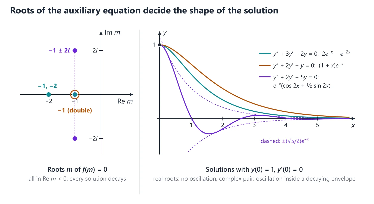
1. Understanding the Operator D and Linearity
Why we need it: springs, pendulums with small swings and electric circuits all lead to equations like ay″ + by′ + cy = X(x) with constant a, b, c. Writing the derivative as an operator D = d/dx turns the left side into a "polynomial in D" acting on y, and polynomials can be factorised, multiplied and divided; this is what makes the whole theory mechanical.
In words: Dy = y′, D2y = y″, and f(D) = a0Dn + ... + an means "take the derivatives and combine them with these constants". The operator is linear: f(D)(c1y1 + c2y2) = c1f(D)y1 + c2f(D)y2. Two consequences follow: sums of solutions of f(D)y = 0 are solutions (superposition), and the difference of two solutions of f(D)y = X solves f(D)y = 0.
First example, slowly: take y″ − y′ − 2y = 0, that is (D2 − D − 2)y = 0. (1) Factorise: D2 − D − 2 = (D − 2)(D + 1); check by expanding (D − 2)(D + 1)y = (D − 2)(y′ + y) = y″ + y′ − 2y′ − 2y = y″ − y′ − 2y.
(2) (D − 2)y = 0 means y′ = 2y, so y = e2x is a solution; since the factors commute, (D + 1)y = 0, that is y = e−x, is also a solution. (3) By linearity y = c1e2x + c2e−x is a solution for all constants, and it has the two constants a second order equation needs.
Non-example: y″ + y2 = 0 is not linear. y = −6/x2 solves it (y″ = −36/x4, y2 = 36/x4), but 2y = −12/x2 gives y″ + y2 = −72/x4 + 144/x4 ≠ 0. Superposition fails, and so do the CF + PI structure and all the operator rules of this topic.
Building up: by the existence and uniqueness theorem for linear equations, each choice of y(x0), y′(x0), ..., y(n−1)(x0) gives exactly one solution of f(D)y = 0. So the solution set is a vector space of dimension n, and n independent solutions (non-zero Wronskian) form a basis; this is why the CF has exactly n constants. Adding one particular solution of f(D)y = X then gives every solution (see "Why y = CF + PI" below).
Where it is used: every equation of this topic and of Laplace transforms; Euler-Cauchy equations reduce to it; in Dynamics it describes free, damped and forced oscillations.
2. Structure of the Solution
Write the equation as f(D)y = X, where D = d/dx and f(D) = a0Dn + a1Dn−1 + ... + an with constants ai, a0 ≠ 0.
Idea: D is an operator, and with constant coefficients f(D) can be factorised and its factors reordered like an ordinary polynomial: (D − a)(D − b) = (D − b)(D − a). With variable coefficients this fails, for example D(xy) = xDy + y, so (D − x)D ≠ D(D − x).
General solution: y = CF + PI, where the complementary function (CF) is the general solution of f(D)y = 0 with n arbitrary constants and the particular integral (PI) is any one solution of f(D)y = X.
Why y = CF + PI: f(D) is linear. If yp is one solution of f(D)y = X and y is any other, then f(D)(y − yp) = X − X = 0, so y − yp belongs to the CF. Conversely CF + yp is always a solution. So every solution is obtained, and the choice of PI does not matter.
The solutions of f(D)y = 0 form an n-dimensional vector space; n solutions form a basis if and only if their Wronskian is non-zero.
Idea: n arbitrary constants match n initial conditions y(x0), y′(x0), ..., y(n−1)(x0); a non-zero Wronskian is exactly what lets these conditions be met uniquely.
3. Understanding the Auxiliary Equation
Why we need it: to write the CF we need n independent solutions of f(D)y = 0. Guessing them one by one is hopeless; the exponential trial y = emx reduces the differential equation to an algebraic equation for m.
In words: since D emx = m emx, f(D)emx = f(m)emx, so emx is a solution exactly when f(m) = 0: this is the auxiliary (characteristic) equation. Each real simple root m gives emx; a root repeated k times gives emx, xemx, ..., xk−1emx; a complex pair α ± iβ gives the two real solutions eαx cos βx and eαx sin βx.
First example, slowly: solve y″ + 4y′ + 13y = 0. (1) Trial y = emx: (m2 + 4m + 13)emx = 0, and emx ≠ 0, so m2 + 4m + 13 = 0. (2) The discriminant is 16 − 52 = −36, so m = (−4 ± 6i)/2 = −2 ± 3i; here α = −2 and β = 3.
(3) The complex solution e(−2 + 3i)x = e−2x(cos 3x + i sin 3x) has real part e−2x cos 3x and imaginary part e−2x sin 3x, and both are real solutions. (4) CF: y = e−2x(c1 cos 3x + c2 sin 3x), a decaying oscillation with angular frequency 3.
(5) A repeated root: y″ − 6y′ + 9y = 0 has m = 3 twice. Check that xe3x works: y′ = e3x(1 + 3x), y″ = e3x(6 + 9x), and y″ − 6y′ + 9y = e3x(6 + 9x − 6 − 18x + 9x) = 0. So the CF is (c1 + c2x)e3x.
Non-example: for the double root m = 3, writing c1e3x + c2e3x is wrong: it equals (c1 + c2)e3x, which has only one essential constant and cannot meet two initial conditions such as y(0) = 0, y′(0) = 1 (the true answer xe3x is missed).
Building up: the three rules are proved in this section below: emx is an eigenfunction of D; for a root of multiplicity k the shift rule gives (D − m)k(xjemx) = emxDkxj = 0 for j less than k; and because f has real coefficients, the real and imaginary parts of a complex solution are real solutions.
Where it is used: the CF of every constant-coefficient equation, the Euler-Cauchy equation after x = ez, the poles of Y(s) in Laplace transforms, and the classification of oscillations (overdamped: real distinct roots, critically damped: double root, underdamped: complex roots).
4. Complementary Function from the Auxiliary Equation f(m) = 0
Real distinct roots m1, ..., mn: CF = c1em1x + ... + cnemnx.
Why it works: D emx = m emx, so f(D)emx = f(m)emx: emx is an "eigenfunction" of D, and it solves f(D)y = 0 exactly when f(m) = 0. Exponentials with distinct m are linearly independent.
Root m repeated k times: contributes (c1 + c2x + ... + ckxk−1)emx.
Why it works: by the shift rule below, (D − m)k(xjemx) = emxDkxj = 0 for j = 0, 1, ..., k − 1, so a root of multiplicity k supplies the k independent solutions emx, xemx, ..., xk−1emx.
Complex pair α ± iβ: eαx(c1 cos βx + c2 sin βx); if the pair is repeated: eαx[(c1 + c2x) cos βx + (c3 + c4x) sin βx].
Why it works: e(α + iβ)x = eαx(cos βx + i sin βx). Since f has real coefficients, the real and imaginary parts of a complex solution are real solutions, and the conjugate root α − iβ gives nothing new.
5. Understanding Inverse Operators 1/f(D)
Why we need it: after the CF we still need one particular solution of f(D)y = X. Writing y = [1/f(D)]X and then manipulating 1/f(D) like a fraction gives short rules for the common right sides (exponentials, sines, polynomials), with no integration at all.
In words: [1/f(D)]X denotes any one function y with f(D)y = X. In particular 1/D means integration (no constant), and [1/(D − a)]X = eax∫e−axX dx, the solution of the linear equation y′ − ay = X. Partial fractions in D are allowed, and for a polynomial X the series expansion of 1/f(D) in powers of D may be used, because only finitely many terms act non-trivially.
First example, slowly: PI of (D2 + 3D + 2)y = e2x. (1) Rule: replace D by 2, since f(D)e2x = f(2)e2x; f(2) = 4 + 6 + 2 = 12 ≠ 0, so PI = e2x/12. (2) Check: y = e2x/12 gives y″ + 3y′ + 2y = (4 + 6 + 2)e2x/12 = e2x.
(3) The same by partial fractions: 1/((D + 1)(D + 2)) = 1/(D + 1) − 1/(D + 2); [1/(D + 1)]e2x = e−x∫e3x dx = e2x/3 and [1/(D + 2)]e2x = e2x/4, so PI = e2x/3 − e2x/4 = e2x/12, the same answer by the slow, always-valid route.
(4) A polynomial right side: [1/(D2 + 1)]x2 = (1 − D2 + D4 − ...)x2 = x2 − 2, the series stopping at D2 because D4x2 = 0. Check: (x2 − 2)″ + (x2 − 2) = 2 + x2 − 2 = x2.
Non-example: for [1/(D2 + 3D + 2)] sin x one may replace D2 by −1 but not D by i. Correctly: 1/(1 + 3D) = (1 − 3D)/(1 − 9D2), and with D2 = −1 this is (1 − 3D)/10, so PI = (sin x − 3 cos x)/10 (check: y″ + 3y′ + 2y = sin x). Putting D = i instead gives the complex number 1/(1 + 3i), which is not an operator on sin x.
Building up: the eax rule, the D2 = −a2 rule and the exponential shift [1/f(D)](eaxV) = eax[1/f(D + a)]V all come from f(D)(eaxV) = eaxf(D + a)V (derived below). The series rule works because f(D)·(truncated series) differs from 1 only by terms of order above m in D, which annihilate xm.
Where it is used: almost every "solve" question on this topic; the same operator algebra solves Euler-Cauchy equations in θ and the simultaneous equations treated later in this topic.
6. Understanding the Failure (Resonance) Case
Why we need it: the short rules divide by f(a) or φ(−a2). When the right side is itself a solution of the homogeneous equation, that number is zero and the rule breaks down. Physically this is resonance: a spring pushed at exactly its natural frequency.
In words: if a is a root of f of multiplicity k, the PI of eax is xkeax/f(k)(a): an extra factor xk appears. For sin ax or cos ax with f(D) = D2 + a2, the PI is −(x/(2a)) cos ax or (x/(2a)) sin ax. In every case the answer grows with x, because the forcing keeps adding energy in step with the natural motion.
First example, slowly: PI of (D2 + 1)y = cos x. (1) Putting D2 = −1 gives the denominator −1 + 1 = 0: failure case. (2) Work with eix, whose real part is cos x: i is a simple root of m2 + 1, with derivative 2i there, so [1/(D2 + 1)]eix = xeix/(2i).
(3) xeix/(2i) = (x/2)(sin x − i cos x), whose real part is (x/2) sin x. (4) Check: y = (x/2) sin x gives y′ = (1/2) sin x + (x/2) cos x and y″ = cos x − (x/2) sin x, so y″ + y = cos x. Notice the amplitude x/2 grows without bound.
(5) The exponential version: (D − 2)2y = e2x has a = 2 as a double root and f″(2) = 2, so PI = x2e2x/2.
Non-example: (D2 + 1)y = cos 2x is not a failure case: D2 = −4 gives the denominator −3 ≠ 0, and PI = −(cos 2x)/3. Multiplying by x here would be wrong; the extra x appears only when the forcing frequency equals a natural frequency (a root of f).
Building up: the annihilator view explains the x: cos x is killed by D2 + 1, so any solution of (D2 + 1)y = cos x also solves (D2 + 1)2y = 0, whose roots ±i are double. The new solutions this brings, x cos x and x sin x, are the only candidates for the PI; the eax formula with f(k)(a) is derived below from f(D) = (D − a)kg(D).
Where it is used: a large share of exam questions are built so that one right-hand term hits the CF; recognising it first saves the whole question. In Dynamics it is the resonance of forced oscillations.
7. Short Methods for the Particular Integral
X = eax: PI = eax/f(a) if f(a) ≠ 0; if a is a root of multiplicity k, PI = xkeax/f(k)(a).
X = sin ax or cos ax: put D2 = −a2; if a factor linear in D remains in the denominator, multiply by its conjugate to bring D2 into the denominator, then put D2 = −a2 again.
Failure case: 1/(D2 + a2) sin ax = −(x/(2a)) cos ax and 1/(D2 + a2) cos ax = (x/(2a)) sin ax.
X = xm: write 1/f(D) as [1 ± φ(D)]−1 (after taking out a constant or a power of D), expand in ascending powers of D up to Dm, and operate on xm.
X = eaxV: PI = eax[1/f(D + a)]V (exponential shift).
X = xV: PI = x[1/f(D)]V − [f′(D)/(f(D))2]V.
General method: 1/(D − a) X = eax∫X e−ax dx; split 1/f(D) into partial fractions and apply this to each term.
8. Derivation: The Exponential Shift and the eax Rule
D(eaxV) = eax(DV + aV) = eax(D + a)V. Repeating, Dn(eaxV) = eax(D + a)nV, and by linearity f(D)(eaxV) = eaxf(D + a)V. Inverting both sides gives [1/f(D)](eaxV) = eax[1/f(D + a)]V.
With V = 1: f(D)eax = f(a)eax, so eax/f(a) is a PI when f(a) ≠ 0.
If a is a root of multiplicity k, write f(D) = (D − a)kg(D) with g(a) ≠ 0. Then [1/f(D)]eax = (1/g(a)) eax(1/Dk)(1) = xkeax/(k! g(a)), and since f(k)(a) = k! g(a) this is xkeax/f(k)(a).
9. Derivation: Trigonometric Right Sides and the Failure Case
D2 sin ax = −a2 sin ax, so φ(D2) sin ax = φ(−a2) sin ax and [1/φ(D2)] sin ax = sin ax/φ(−a2) when φ(−a2) ≠ 0; the same holds for cos ax. This is why D2 may be replaced by −a2, but D itself may not.
Failure case: ia is a simple root of D2 + a2, with derivative 2ia there, so [1/(D2 + a2)]eiax = xeiax/(2ia) = (x/(2a))(sin ax − i cos ax).
Taking real and imaginary parts: [1/(D2 + a2)] cos ax = (x/(2a)) sin ax and [1/(D2 + a2)] sin ax = −(x/(2a)) cos ax, the formulas stated above.
General rule: (D − a)y = X is a linear first order equation with IF e−ax, which gives [1/(D − a)]X = eax∫Xe−ax dx; with partial fractions this handles any X, at the cost of an integration.
10. Choosing the Method
If X = eax → eax/f(a); if f(a) = 0 → multiply by xk and divide by f(k)(a).
If X = sin ax or cos ax → D2 = −a2, rationalising any leftover linear factor; if the denominator vanishes → failure-case formula, or work with eiax and take the real or imaginary part.
If X is a polynomial → take out the lowest power of D, expand [1 ± φ(D)]−1 only up to the degree of the polynomial.
If X = eax × (polynomial or trigonometric) → exponential shift; if X = xm sin ax → write it as the imaginary part of xmeiax and shift.
If X is sec ax, tan ax, cosec ax, log x, 1/x or similar → the short methods do not apply: use partial fractions with eax∫Xe−ax dx, or variation of parameters.
If initial conditions are given and the question says "by Laplace transform" → use the Laplace method of the next topic.
11. Common Mistakes
Forgetting that the forcing term may solve the homogeneous equation: using eax/f(a) or D2 = −a2 when the denominator is zero, instead of multiplying by x.
Complex roots α ± iβ: writing eαx(c1 cos iβx + ...) or taking β = (discriminant)/2 instead of √|discriminant|/(2a0).
Substituting D = ia (or D = a) in a leftover odd power of D when X is trigonometric; the denominator must first be rationalised so that only D2 remains to be replaced by −a2.
In undetermined coefficients, using a trial function with missing terms (only sin bx when both sin bx and cos bx are needed, or an incomplete polynomial).
For simultaneous equations, introducing new constants when finding the second unknown from the first, which gives more constants than the degree of the operator determinant.
12. Connections
Link: the solution space of f(D)y = 0 is the null space of a linear operator, of dimension n (Linear Algebra); Laplace transforms solve the same equations with the initial conditions built in, and the roots of the auxiliary equation are the poles of the transformed solution.
Link: the failure case is resonance in Dynamics: x″ + ω2x = F cos ωt has the PI (Ft/(2ω)) sin ωt, whose amplitude grows linearly with time (simple harmonic motion and forced oscillations).
13. Worked Examples
Example 1: Solve (D2 − 3D + 2)y = e3x.
m2 − 3m + 2 = 0 gives m = 1, 2; PI = e3x/(9 − 9 + 2) = e3x/2; y = c1ex + c2e2x + e3x/2.
Example 2: Solve (D2 + 4)y = sin 2x.
CF = c1 cos 2x + c2 sin 2x; D2 = −4 makes the denominator zero, so PI = −(x/4) cos 2x.
Example 3: Solve (D2 + D)y = x2 + 2x + 4.
CF = c1 + c2e−x; PI = (1/D)(1 + D)−1(x2 + 2x + 4) = (1/D)[(x2 + 2x + 4) − (2x + 2) + 2] = (1/D)(x2 + 4) = x3/3 + 4x.
Example 4: Solve (D − 1)2y = xex.
CF = (c1 + c2x)ex; PI = ex(1/D2)x = x3ex/6.
Example 5 (third order): Solve (D3 − 1)y = 0.
m3 = 1 gives m = 1, (−1 ± i√3)/2, so y = c1ex + e−x/2[c2 cos(√3x/2) + c3 sin(√3x/2)].
Example 6: Solve (D2 − 2D + 5)y = ex cos 2x.
m2 − 2m + 5 = 0 gives m = 1 ± 2i, so CF = ex(c1 cos 2x + c2 sin 2x).
Exponential shift: PI = ex[1/((D + 1)2 − 2(D + 1) + 5)] cos 2x = ex[1/(D2 + 4)] cos 2x = ex(x/4) sin 2x (failure case).
Hence y = ex(c1 cos 2x + c2 sin 2x) + (x/4)ex sin 2x.
Example 7: Solve (D3 − D2 − D + 1)y = cosh x.
f(m) = (m − 1)2(m + 1), so CF = (c1 + c2x)ex + c3e−x; write cosh x = (ex + e−x)/2.
a = 1 is a double root and f″(1) = 6 − 2 = 4, so (1/2)[1/f(D)]ex = x2ex/8; a = −1 is a simple root and f′(−1) = 3 + 2 − 1 = 4, so (1/2)[1/f(D)]e−x = xe−x/8.
Hence y = (c1 + c2x)ex + c3e−x + (x2ex + xe−x)/8.
Initial conditions are applied to the complete solution y = CF + PI, never to the CF alone.
14. Simultaneous Equations, Undetermined Coefficients and Initial Values
Simultaneous linear equations f1(D)x + g1(D)y = X1, f2(D)x + g2(D)y = X2: eliminate y by operating with g2(D) and g1(D) and subtracting (D commutes with constants), solve for x, then find y from one of the equations without adding new constants. The number of arbitrary constants equals the degree in D of f1g2 − f2g1.
Undetermined coefficients: for X a polynomial, eax, sin bx, cos bx or their products, try a combination of the same form (multiplied by xk if the trial form solves f(D)y = 0) and equate coefficients.
Why undetermined coefficients works: each admissible X is itself a solution of some constant-coefficient equation g(D)X = 0 (its annihilator, for example D2 + b2 for sin bx). Then g(D)f(D)y = 0, so the PI is a combination of the solutions of g(D)f(D)y = 0 that are not already in the CF; the factor xk appears when g and f share a root.
Example 8 (UPSC 2017, 8 marks): (i) Solve the following simultaneous linear differential equations:
(D + 1)y = z + ex and (D + 1)z = y + ex where y and z are functions of independent variable x and D ≡ d/dx.
Subtracting the equations: (D + 1)(y − z) = z − y, that is (D + 2)(y − z) = 0, so y − z = Ae−2x.
Adding: (D + 1)(y + z) = (y + z) + 2ex, that is D(y + z) = 2ex, so y + z = 2ex + B.
Answer: y = ex + B/2 + (A/2)e−2x, z = ex + B/2 − (A/2)e−2x (two arbitrary constants, as the determinant (D + 1)2 − 1 has degree 2).
Example 9 (UPSC 2017, 7 marks): (ii) Solve the following initial value differential equations:
20y″ + 4y′ + y = 0, y(0) = 3·2 and y′(0) = 0.
Auxiliary equation 20m2 + 4m + 1 = 0: m = (−4 ± √(16 − 80))/40 = −1/10 ± i/5, so y = e−x/10(A cos(x/5) + B sin(x/5)).
y(0) = A = 3.2 (written 3·2 in the paper) and y′(0) = −A/10 + B/5 = 0, so B = 1.6.
Answer: y = e−0.1x(3.2 cos 0.2x + 1.6 sin 0.2x).
15. Practice Exercises
Exercise 1 (basic): Solve y″ − 5y′ + 6y = 0.
Answer: m = 2, 3; y = c1e2x + c2e3x.
Exercise 2 (basic): Solve y″ + 2y′ + 5y = 0.
Answer: m = −1 ± 2i; y = e−x(c1 cos 2x + c2 sin 2x).
Exercise 3 (basic): Solve (D3 − 3D2 + 3D − 1)y = 0.
Answer: (m − 1)3 = 0, a triple root; y = (c1 + c2x + c3x2)ex.
Exercise 4 (standard): Solve (D2 + 4D + 4)y = e−2x.
Answer: −2 is a double root and f″ = 2, so y = (c1 + c2x)e−2x + x2e−2x/2.
Exercise 5 (standard): Solve (D2 + 9)y = cos 3x + sin x.
Answer: y = c1 cos 3x + c2 sin 3x + (x/6) sin 3x + (sin x)/8 (the first term is the failure case).
Exercise 6 (standard): Find a particular integral of (D2 − D − 2)y = x2.
Answer: PI = −(1/2)[1 + (D − D2)/2]−1x2 = −x2/2 + x/2 − 3/4.
Exercise 7 (standard): Find a particular integral of (D2 + 2D + 2)y = e−x sin x.
Answer: the shift D → D − 1 gives e−x[1/(D2 + 1)] sin x, so PI = −(x/2)e−x cos x.
Exercise 8 (UPSC level): Solve (D2 + 1)y = x sin x.
Answer: take the imaginary part of [1/(D2 + 1)](xeix) = eix[1/(D2 + 2iD)]x; y = c1 cos x + c2 sin x + (x sin x − x2 cos x)/4.
Exercise 9 (UPSC level): Solve y″ + 4y = 8 cos 2x, y(0) = 0, y′(0) = 2.
Answer: y = c1 cos 2x + c2 sin 2x + 2x sin 2x; the conditions give c1 = 0, c2 = 1, so y = (1 + 2x) sin 2x (resonance: the amplitude grows linearly).
Exercise 10 (UPSC level): Solve dx/dt + y = sin t, dy/dt + x = cos t with x(0) = 2, y(0) = 0.
Answer: eliminating y gives (D2 − 1)x = 0, so x = Aet + Be−t and y = sin t − Aet + Be−t; the conditions give A = B = 1: x = 2 cosh t, y = sin t − 2 sinh t.
| X | PI = [1/f(D)]X | Condition |
|---|---|---|
| eax | eax/f(a) | f(a) ≠ 0 |
| eax | xeax/f′(a) | f(a) = 0, f′(a) ≠ 0 |
| sin ax, cos ax | Put D2 = −a2 | Denominator ≠ 0 |
| sin ax | −(x/(2a)) cos ax | f(D) = D2 + a2 |
| cos ax | (x/(2a)) sin ax | f(D) = D2 + a2 |
| xm | Expand [f(D)]−1 up to Dm | Take out a power of D if f(0) = 0 |
| eaxV | eax[1/f(D + a)]V | Always |
| xV | x[1/f(D)]V − [f′(D)/(f(D))2]V | Always |
Mains points
- Questions usually combine several right-hand terms (such as ex + sin 2x + x2); find the PI of each term separately and add.
- Check the failure case first: if eax or sin ax already appears in the CF, the PI carries an extra factor x.
- For xm, stop the series at Dm; when f(0) = 0, take out the factor D before expanding.
- Present the answer as y = CF + PI with the auxiliary roots shown; the CF earns marks even if the PI slips.
- For initial value problems, substitute conditions only after writing the complete solution, and verify the final answer.
Did you know?
- Euler introduced the trial solution y = emx in the 1740s; it turns a linear ODE with constant coefficients into the algebraic auxiliary equation f(m) = 0.
Second Order Equations with Variable Coefficients
The Euler-Cauchy equation becomes one with constant coefficients under x = ez. If one solution y1 of y″ + Py′ + Qy = 0 is known, y = vy1 reduces the order. Variation of parameters gives the particular integral for any R(x) once two independent solutions are known.
1. Understanding the Euler-Cauchy Substitution
Why we need it: once the coefficients depend on x, the trial emx no longer works, and there is no general recipe. One important family is still easy: equations in which each derivative y(k) is multiplied by a constant times xk. They arise when Laplace's equation is separated in polar or spherical coordinates.
In words: in x2y″ + axy′ + by = X the factor xk "matches" the k-th derivative, so the equation does not change when x is scaled to λx. The substitution x = ez turns scaling into shifting (log λx = log λ + z), and shift-invariant equations are exactly those with constant coefficients. In the new variable, xD becomes θ = d/dz and x2D2 becomes θ(θ − 1).
First example, slowly: solve x2y″ − 2xy′ + 2y = 0 for x > 0. (1) Trial y = xm: y′ = mxm−1, y″ = m(m − 1)xm−2, so x2y″ = m(m − 1)xm and xy′ = mxm. (2) Substituting: [m(m − 1) − 2m + 2]xm = 0, that is m2 − 3m + 2 = 0, so m = 1, 2.
(3) The general solution is y = c1x + c2x2. (4) Check y = x2: 2x2 − 4x2 + 2x2 = 0. (5) The same result through x = ez: [θ(θ − 1) − 2θ + 2]y = (θ − 1)(θ − 2)y = 0 gives y = c1ez + c2e2z = c1x + c2x2; the indicial polynomial in m is the auxiliary polynomial in θ.
Non-example: x2y″ + y′ + y = 0 is not of Euler-Cauchy type, because y′ is multiplied by 1, not by a constant times x. With x = ez it becomes θ(θ − 1)y + e−zθy + y = 0, which still has a variable coefficient e−z, so the method gives nothing.
Building up: from dy/dx = (1/x) dy/dz we get xD = θ; differentiating once more, x2D2 = θ2 − θ = θ(θ − 1), and by induction xkDk = θ(θ − 1)...(θ − k + 1) (shown in this section). The right side X(x) must also be rewritten in z; then every PI rule of the constant-coefficient topic applies in θ. Legendre's equation (ax + b)ky(k) works the same way with ax + b = ez.
Where it is used: a 10–15 mark Euler-Cauchy or Legendre-type question appears almost every year; the same equation r2R″ + rR′ − n2R = 0 gives the radial part of Laplace's equation in a disc.
2. Euler-Cauchy (Homogeneous Linear) Equation
Form: xny(n) + a1xn−1y(n−1) + ... + any = X(x), with constants ai, for x > 0.
Put x = ez (z = log x) and θ = d/dz: xD = θ, x2D2 = θ(θ − 1), x3D3 = θ(θ − 1)(θ − 2).
Why it works: with x = ez, dy/dx = (dy/dz)(dz/dx) = (1/x) dy/dz, so x dy/dx = θy. Differentiating again, x2 d2y/dx2 = d2y/dz2 − dy/dz = θ(θ − 1)y, and in general xkDk = θ(θ − 1)...(θ − k + 1).
The equation becomes linear with constant coefficients in z; solve it and put back z = log x.
Idea: xm plays the role that emx plays for constant coefficients: (xD)xm = m xm. So for the homogeneous equation x2y″ + axy′ + by = 0 the trial y = xm gives m(m − 1) + am + b = 0 directly; a double root m gives xm and xm log x, and complex roots α ± iβ give xα[c1 cos(β log x) + c2 sin(β log x)]. For x < 0 use x = −ez, that is replace x by |x|.
Legendre's linear equation (ax + b)ny(n) + ... = X: put ax + b = ez; then (ax + b)D = aθ, (ax + b)2D2 = a2θ(θ − 1).
Example 1: Solve x2y″ − 2xy′ − 4y = x4.
With x = ez: [θ(θ − 1) − 2θ − 4]y = e4z, that is (θ − 4)(θ + 1)y = e4z.
CF = c1e4z + c2e−z; since 4 is a simple root of f(θ) = θ2 − 3θ − 4, PI = ze4z/f′(4) = ze4z/5.
Hence y = c1x4 + c2/x + (x4 log x)/5.
3. Understanding Reduction of Order
Why we need it: for a general second order linear equation we cannot find the CF from an auxiliary equation. But very often one solution can be spotted (y = x, y = ex, y = xm), and one known solution is enough to find everything else.
In words: if y1 solves y″ + Py′ + Qy = 0, look for other solutions in the form y = v(x)y1(x), letting the "constant" multiplier vary. Because y1 already solves the equation, all terms containing v itself cancel, leaving only v′ and v″: a first order linear equation for w = v′. That is why the order is "reduced".
First example, slowly: (1 − x2)y″ − 2xy′ + 2y = 0 on −1 < x < 1. (1) Standard form: P = −2x/(1 − x2), Q = 2/(1 − x2). (2) Test y = x: P + Qx = −2x/(1 − x2) + 2x/(1 − x2) = 0, so y1 = x.
(3) ∫P dx = log(1 − x2), so e−∫P dx = 1/(1 − x2). (4) y2 = y1∫e−∫P dx/y12 dx = x∫dx/(x2(1 − x2)) = x∫[1/x2 + 1/(1 − x2)] dx.
(5) Integrating, y2 = x[−1/x + (1/2) log((1 + x)/(1 − x))] = (x/2) log((1 + x)/(1 − x)) − 1. (6) The general solution is c1x + c2[(x/2) log((1 + x)/(1 − x)) − 1]; this is Legendre's equation of degree 1, and y2 is the function usually called Q1(x).
Non-example: for the same equation, the rule 1 + P + Q = 0 for ex fails: 1 + (2 − 2x)/(1 − x2) = 1 + 2/(1 + x) ≠ 0. So ex is not a solution, and putting y = vex would not remove the v-terms. The inspection rules must be checked, not assumed.
Building up: with y = vy1, the v-terms collect into v(y1″ + Py1′ + Qy1) = 0, leaving y1v″ + (2y1′ + Py1)v′ = R. Its IF is y12e∫P dx, which gives the formula y2 = y1∫e−∫P dx/y12 dx when R = 0 and the CF and PI together when R ≠ 0 (both derived in this section).
Where it is used: "given that y = x (or ex) is a solution, solve ..." and "find the second solution" questions; it also supplies the y2 needed before variation of parameters.
4. Complete Solution When One Solution Is Known
Standard form: y″ + P(x)y′ + Q(x)y = R(x) (coefficient of y″ equal to 1).
If y1 is a known non-zero solution of y″ + Py′ + Qy = 0, put y = vy1; then v″ + (P + 2y1′/y1)v′ = R/y1, a first order linear equation in v′.
Why it works: with y = vy1, y′ = v′y1 + vy1′ and y″ = v″y1 + 2v′y1′ + vy1″. Substituting, the terms in v collect into v(y1″ + Py1′ + Qy1) = 0, leaving v″y1 + v′(2y1′ + Py1) = R; divide by y1. Because v itself has disappeared, w = v′ satisfies a first order equation: the order is reduced.
Second independent solution of the homogeneous equation: y2 = y1∫[e−∫P dx/y12] dx.
Why it works: with R = 0, w′ + (P + 2y1′/y1)w = 0 has IF y12e∫P dx, so w = e−∫P dx/y12 and v = ∫w dx.
Finding y1 by inspection: 1 + P + Q = 0 ⇒ ex; 1 − P + Q = 0 ⇒ e−x; a2 + aP + Q = 0 ⇒ eax; P + Qx = 0 ⇒ x; 2 + 2Px + Qx2 = 0 ⇒ x2; m(m − 1) + Pmx + Qx2 = 0 ⇒ xm.
Why the rules work: substitute the trial function in y″ + Py′ + Qy = 0. For y = eax: (a2 + aP + Q)eax = 0. For y = x: P + Qx = 0. For y = xm: m(m − 1)xm−2 + Pmxm−1 + Qxm = 0, which is the stated condition after multiplying by x2 − m. Always verify the guessed y1 in the given equation.
Example 2: Solve x2y″ − (x2 + 2x)y′ + (x + 2)y = x3ex.
Standard form: P = −(1 + 2/x), Q = (x + 2)/x2, R = xex; P + Qx = 0, so y1 = x.
With y = vx: v″ + (P + 2/x)v′ = ex, that is v″ − v′ = ex; then v′ = (x + c1)ex and v = (x − 1)ex + c1ex + c2.
Hence y = c1xex + c2x + x(x − 1)ex, which can be written y = Axex + Bx + x2ex.
5. Understanding the Wronskian
Why we need it: the CF needs two solutions that are genuinely different, not multiples of each other. For two functions this is easy to see, but we need a test that also works for n functions and that can be computed mechanically.
In words: y1, y2 are linearly dependent on an interval if c1y1 + c2y2 = 0 there for constants not both zero. Their Wronskian is W = y1y2′ − y2y1′, the determinant of [[y1, y2], [y1′, y2′]]. If the functions are dependent, W ≡ 0. For two solutions of y″ + Py′ + Qy = 0 with continuous P, Q, the converse also holds, and W is either never zero or identically zero (Abel's formula).
First example, slowly: y1 = cos x, y2 = sin x, solutions of y″ + y = 0. (1) y1′ = −sin x, y2′ = cos x. (2) W = cos x·cos x − sin x·(−sin x) = 1. (3) W ≠ 0, so they are independent and y = c1 cos x + c2 sin x is the general solution. (4) Abel agrees: here P = 0, so W = Ce0 is constant.
Non-example: x2 and x|x| on (−1, 1) are independent (no single constant ratio works on both sides of 0), yet their Wronskian is identically zero. This does not contradict the theorem: they cannot both be solutions of one equation y″ + Py′ + Qy = 0 with P, Q continuous on (−1, 1). "W ≡ 0 implies dependence" is true only for solutions of such an equation.
Building up: if W(x0) = 0, the system c1y1(x0) + c2y2(x0) = 0, c1y1′(x0) + c2y2′(x0) = 0 has a non-zero solution; then c1y1 + c2y2 solves the equation with zero initial data, so by uniqueness it is identically zero. Abel's formula W = Ce−∫P dx (proved in the Wronskian section below) shows that W cannot vanish at one point without vanishing everywhere.
Where it is used: W is the denominator of the variation of parameters formula, the test of a fundamental set of solutions, and the determinant behind Cramer's rule in the derivation below; in Linear Algebra it is a test of linear independence in a function space.
6. Understanding Variation of Parameters
Why we need it: the short operator methods work only for special right sides (eax, sin ax, polynomials) and only for constant coefficients. For R(x) = sec x, tan x, ex/x or for variable coefficients we need a method that gives the PI for any continuous R, once the CF is known.
In words: the CF is c1y1 + c2y2. We let the constants vary, y = u1(x)y1 + u2(x)y2, and choose u1, u2 so that the equation is satisfied. Two unknown functions need two conditions: the equation itself, and the convenient extra condition u1′y1 + u2′y2 = 0. Solving gives u1′ = −y2R/W and u2′ = y1R/W, with R read from the standard form.
First example, slowly: test the method on y″ + y = x, whose PI x is known. (1) y1 = cos x, y2 = sin x, W = 1, R = x. (2) u1 = −∫x sin x dx = x cos x − sin x. (3) u2 = ∫x cos x dx = x sin x + cos x.
(4) PI = u1y1 + u2y2 = x cos2x − sin x cos x + x sin2x + sin x cos x = x. (5) The method reproduces the known answer; for R = sec x the same steps give the PI cos x log|cos x| + x sin x (Example 3), where no short method exists.
Non-example: x2y″ − 2xy′ + 2y = x3 with y1 = x, y2 = x2, W = x2. Taking R = x3 (without dividing by x2) gives u1 = −x4/4, u2 = x2/2 and the "PI" −x5/4 + x4/2, which does not satisfy the equation. With the correct R = x: u1 = −x2/2, u2 = x, and PI = x3/2, which does.
Building up: the extra condition makes y′ = u1y1′ + u2y2′ free of u′, so y″ contains only first derivatives of u1, u2; substituting, the CF parts cancel and u1′y1′ + u2′y2′ = R remains. The 2 × 2 system has determinant W ≠ 0, and Cramer's rule gives the formulas (full derivation below). Constants of integration in u1, u2 simply reproduce the CF.
Where it is used: questions that say "by the method of variation of parameters" (15–20 marks, very frequent), right sides like sec x, cosec x, tan x, ex/x, and the first order case y′ + Py = Q of the first topic.
7. Method of Variation of Parameters
Let y1, y2 be independent solutions of y″ + Py′ + Qy = 0 with Wronskian W = y1y2′ − y2y1′ ≠ 0.
Seek y = u1y1 + u2y2 with u1′y1 + u2′y2 = 0 and u1′y1′ + u2′y2′ = R.
Why the extra condition: one equation cannot fix two unknown functions u1, u2, so we are free to impose one more condition. Choosing u1′y1 + u2′y2 = 0 makes y′ = u1y1′ + u2y2′ free of u′, so that y″ contains only first derivatives of u1, u2.
Solving: u1 = −∫(y2R/W) dx, u2 = ∫(y1R/W) dx, so PI = −y1∫(y2R/W) dx + y2∫(y1R/W) dx.
The method needs the standard form and works for any continuous R(x), including sec x, tan x and cosec x, where the short methods fail.
Example 3: Solve y″ + y = sec x by variation of parameters.
y1 = cos x, y2 = sin x, W = 1; u1 = −∫sin x sec x dx = log|cos x|, u2 = ∫cos x sec x dx = x.
Hence y = c1 cos x + c2 sin x + cos x log|cos x| + x sin x.
8. Understanding the Normal Form
Why we need it: the first derivative term Py′ is what stops many equations from looking like the simple u″ + ku = 0. A clever change of the dependent variable can remove it, and if what remains has a constant coefficient the equation is solved at once.
In words: put y = uv with v = e−(1/2)∫P dx. Then y″ + Py′ + Qy = R becomes u″ + Iu = R/v, the normal form, with the invariant I = Q − P2/4 − P′/2. The method pays off when I is a constant (or c/x2, which gives an Euler-Cauchy equation).
First example, slowly: y″ + (2/x)y′ + y = 0. (1) P = 2/x, so v = e−∫dx/x = 1/x. (2) I = Q − P2/4 − P′/2 = 1 − 1/x2 + 1/x2 = 1. (3) u″ + u = 0 gives u = c1 cos x + c2 sin x. (4) y = uv = (c1 cos x + c2 sin x)/x; check y = (sin x)/x directly if you like.
Non-example: for y″ + xy′ + y = 0, I = 1 − x2/4 − 1/2 = 1/2 − x2/4 is not constant, so the normal form u″ + (1/2 − x2/4)u = 0 is no easier. (This equation is exact instead: P0″ − P1′ + P2 = 0 − 1 + 1 = 0.) Always compute I before committing to the method.
Building up: with y = uv the coefficient of u′ is 2v′ + Pv, which vanishes for v = e−(1/2)∫P dx; the remaining coefficient of u is v″ + Pv′ + Qv = Iv (derived in this section). The companion trick, changing the independent variable to z with (z′)2 proportional to Q, makes Q1 constant and works when P1 = (z″ + Pz′)/(z′)2 also turns out constant.
Where it is used: "reduce to normal form and solve" questions, Bessel-type equations such as y″ + (2/x)y′ + y = 0, and checking whether a change of independent variable will work.
9. Related Reductions
Normal form: y = uv with v = e−(1/2)∫P dx removes the first derivative and gives u″ + Iu = R/v, where I = Q − P2/4 − P′/2.
Why it works: with y = uv, the coefficient of u′ in y″ + Py′ + Qy is 2v′ + Pv; it vanishes for v = e−(1/2)∫P dx. Then v′ = −Pv/2 and v″ = (P2/4 − P′/2)v, and the coefficient of u becomes v″ + Pv′ + Qv = (Q − P2/4 − P′/2)v = Iv. The method helps when I is a constant or a constant divided by x2.
Change of independent variable z = z(x): the equation becomes d2y/dz2 + P1dy/dz + Q1y = R1 with P1 = (z″ + Pz′)/(z′)2, Q1 = Q/(z′)2, R1 = R/(z′)2; choose z so that Q1 is constant and check that P1 is then constant.
Why it works: dy/dx = z′ dy/dz and d2y/dx2 = (z′)2 d2y/dz2 + z″ dy/dz; substituting and dividing by (z′)2 gives P1, Q1, R1. Making Q1 constant means (z′)2 ∝ Q, that is z = ∫√|Q| dx (up to a constant factor); for xy″ − y′ + 4x3y = x5 this gives z = x2.
10. Derivation: The Variation of Parameters Formula
Seek y = u1y1 + u2y2 with u1′y1 + u2′y2 = 0. Then y′ = u1y1′ + u2y2′ and y″ = u1y1″ + u2y2″ + u1′y1′ + u2′y2′.
Substituting in y″ + Py′ + Qy = R, the terms u1(y1″ + Py1′ + Qy1) and u2(y2″ + Py2′ + Qy2) vanish, leaving u1′y1′ + u2′y2′ = R.
The two equations form the system [[y1, y2], [y1′, y2′]](u1′, u2′)T = (0, R)T, whose determinant is the Wronskian W ≠ 0.
By Cramer's rule u1′ = −y2R/W and u2′ = y1R/W. Integrating gives the formula; the constants of integration reproduce the CF, so writing them in gives the complete solution in one step.
11. Choosing the Method
If each y(k) is multiplied by a constant times xk → Euler-Cauchy, x = ez (or y = xm for the homogeneous part); if by (ax + b)k → Legendre, ax + b = ez.
If one of the inspection rules gives y1 → reduction of order y = vy1, which gives the CF and the PI together.
If two independent solutions are known and R is arbitrary (sec x, tan x, ex/x, log x), or the question says "by variation of parameters" → variation of parameters.
If I = Q − P2/4 − P′/2 is a constant (or c/x2) → normal form; if Q/(z′)2 can be made constant with P1 also constant → change of independent variable.
If P0″ − P1′ + P2 = 0 → exact: write down the first integral. If y is absent → p = y′; if x is absent → p = y′ with y″ = p dp/dy.
12. Common Mistakes
Writing x2D2 = θ2 instead of θ(θ − 1) in the Euler-Cauchy reduction.
Leaving the right side in x after putting x = ez; it must also be rewritten in z (log x = z, xn = enz) before any operator method is applied.
Using a y1 that solves only part of the equation, or one found from the rules with P, Q read before dividing by the coefficient of y″.
Dropping the minus sign in u1 = −∫y2R/W dx, or forgetting to divide by W.
In the normal form, solving for u and forgetting to multiply by v at the end: the answer is y = uv.
13. Connections
Link: the Euler-Cauchy equation r2R″ + rR′ − n2R = 0 appears when Laplace's equation is separated in polar coordinates (Partial Differential Equations), and the first order variation of parameters in topic 1 is the n = 1 case of the formula derived here.
Link: the Wronskian tests linear independence of functions (Linear Algebra); for a system Y′ = AY its analogue is Liouville's formula W = Ce∫tr A dx, of which Abel's formula is the case A = [[0, 1], [−Q, −P]].
14. Worked Examples
Example 4: Solve x2y″ − xy′ + y = log x.
With x = ez: [θ(θ − 1) − θ + 1]y = z, that is (θ − 1)2y = z; CF = (c1 + c2z)ez.
PI = (1 − θ)−2z = (1 + 2θ + 3θ2 + ...)z = z + 2.
Hence y = (c1 + c2 log x)x + log x + 2.
Example 5: Solve y″ − 2y′ + y = ex/x by variation of parameters.
y1 = ex, y2 = xex, W = e2x, R = ex/x.
u1 = −∫xex(ex/x)/e2x dx = −x and u2 = ∫ex(ex/x)/e2x dx = log x.
PI = −xex + xex log x; absorbing −xex into the CF, y = (c1 + c2x)ex + xex log x (x > 0).
Example 6: Solve y″ − 4xy′ + (4x2 − 1)y = −3ex2 sin 2x by reducing to normal form.
P = −4x, so v = e−(1/2)∫P dx = ex2 and I = Q − P2/4 − P′/2 = (4x2 − 1) − 4x2 + 2 = 1.
With y = uex2: u″ + u = R/v = −3 sin 2x, so u = c1 cos x + c2 sin x − 3 sin 2x/(1 − 4) = c1 cos x + c2 sin x + sin 2x.
Hence y = ex2(c1 cos x + c2 sin x + sin 2x).
Example 7: Solve xy″ − y′ + 4x3y = x5 by changing the independent variable.
Standard form: y″ − y′/x + 4x2y = x4, so P = −1/x, Q = 4x2, R = x4; take (z′)2 = Q/4 = x2, that is z = x2.
Then P1 = (z″ + Pz′)/(z′)2 = (2 − 2)/(4x2) = 0, Q1 = 4x2/(4x2) = 1 and R1 = x4/(4x2) = z/4.
d2y/dz2 + y = z/4 gives y = c1 cos z + c2 sin z + z/4, that is y = c1 cos x2 + c2 sin x2 + x2/4.
15. Wronskian, Exact Equations and Euler-Cauchy Past Questions
Wronskian and Abel's formula: for solutions y1, y2 of y″ + Py′ + Qy = 0 on an interval where P, Q are continuous, W = y1y2′ − y2y1′ = Ce−∫P dx; so W is either identically 0 (dependent solutions) or never 0 (independent).
Why Abel's formula holds: W′ = y1y2″ − y2y1″ = y1(−Py2′ − Qy2) − y2(−Py1′ − Qy1) = −PW, a separable equation with solution W = Ce−∫P dx. Since an exponential never vanishes, W is zero everywhere (C = 0) or nowhere.
Exact equation P0y″ + P1y′ + P2y = R is exact if P0″ − P1′ + P2 = 0; its first integral is P0y′ + (P1 − P0′)y = ∫R dx + c.
Why the exactness condition: d/dx[P0y′ + (P1 − P0′)y] = P0y″ + P1y′ + (P1′ − P0″)y. This equals the left side of the equation exactly when P2 = P1′ − P0″, that is P0″ − P1′ + P2 = 0.
Equation free of y: if y itself is absent, put p = dy/dx to lower the order by one.
Example 8 (UPSC 2016, 15 marks): Find the general solution of the equation x2 d3y/dx3 − 4x d2y/dx2 + 6 dy/dx = 4.
y does not occur, so put p = y′: x2p″ − 4xp′ + 6p = 4, an Euler-Cauchy equation in p.
With x = ez: [θ(θ − 1) − 4θ + 6]p = (θ − 2)(θ − 3)p = 4, so p = c1x2 + c2x3 + 4/6.
Answer: y = Ax3 + Bx4 + 2x/3 + C (A = c1/3, B = c2/4).
Example 9 (UPSC 2018, 13 marks): Solve : (1 + x)2 y″ + (1 + x) y′ + y = 4 cos(log(1 + x))
Legendre's equation: put 1 + x = ez, so (1 + x)D = θ and (1 + x)2D2 = θ(θ − 1). Then [θ(θ − 1) + θ + 1]y = (θ2 + 1)y = 4 cos z.
CF = c1 cos z + c2 sin z; failure case PI = 4·(z/2) sin z = 2z sin z.
Answer: y = c1 cos log(1 + x) + c2 sin log(1 + x) + 2 log(1 + x) sin log(1 + x).
Example 10 (UPSC 2020, 10 marks): (i) Solve the following differential equation : (x + 1)2y″ − 4(x + 1)y′ + 6y = 6(x + 1)2 + sin log(x + 1)
Put x + 1 = ez: [θ(θ − 1) − 4θ + 6]y = (θ − 2)(θ − 3)y = 6e2z + sin z; CF = c1(x + 1)2 + c2(x + 1)3.
θ = 2 is a simple root of f(θ) = θ2 − 5θ + 6, with f′(2) = −1, so PI1 = 6ze2z/(−1) = −6ze2z.
PI2 = [1/(5 − 5θ)] sin z = (1/5)(1 + θ) sin z/(1 − θ2) = (sin z + cos z)/10.
Answer: y = c1(x + 1)2 + c2(x + 1)3 − 6(x + 1)2 log(x + 1) + [sin log(x + 1) + cos log(x + 1)]/10.
Example 11 (UPSC 2022, 10 marks): (ii) Solve the following differential equation: (3x + 2)2 d2y/dx2 + 5(3x + 2) dy/dx − 3y = x2 + x + 1
Put 3x + 2 = ez: (3x + 2)D = 3θ, (3x + 2)2D2 = 9θ(θ − 1). The operator is 9θ(θ − 1) + 15θ − 3 = 3(3θ − 1)(θ + 1), so CF = c1(3x + 2)1/3 + c2(3x + 2)−1.
With x = (ez − 2)/3: x2 + x + 1 = (e2z − ez + 7)/9. For f(θ) = 9θ2 + 6θ − 3: f(2) = 45, f(1) = 12, f(0) = −3.
PI = (1/9)[e2z/45 − ez/12 + 7/(−3)] = e2z/405 − ez/108 − 7/27.
Answer: y = c1(3x + 2)1/3 + c2(3x + 2)−1 + (3x + 2)2/405 − (3x + 2)/108 − 7/27.
Example 12 (UPSC 2025, 10 marks): (ii) Find the complete solution of x3 d3y/dx3 + 3x2 d2y/dx2 + x dy/dx + y = x log x.
With x = ez the operator is θ3 + 1 (as in Problem 9 of the Solved Problems), so CF = c1/x + √x[c2 cos((√3/2) log x) + c3 sin((√3/2) log x)].
PI = [1/(θ3 + 1)] zez = ez[1/((θ + 1)3 + 1)] z = ez[1/(2 + 3θ + 3θ2 + θ3)] z = (ez/2)(1 − 3θ/2)z = (ez/2)(z − 3/2).
Answer: y = c1/x + √x[c2 cos((√3/2) log x) + c3 sin((√3/2) log x)] + (x/2)(log x − 3/2).
Example 13 (UPSC 2026, 15 marks): Solve x2 d2y/dx2 − 3x dy/dx + y = ((sin(log x) + 1)/x) log x.
With x = ez: (θ2 − 4θ + 1)y = e−zz(sin z + 1). Roots θ = 2 ± √3, so CF = c1x2 + √3 + c2x2 − √3.
Exponential shift: PI = e−z[1/f(θ)](z sin z + z), where f(θ) = (θ − 1)2 − 4(θ − 1) + 1 = θ2 − 6θ + 6.
[1/f(θ)]z = (1/6)(1 + θ + ...)z = (z + 1)/6.
For z sin z use [1/f]zV = z[1/f]V − [f′/f2]V with V = sin z. With θ2 = −1, f = 5 − 6θ, so [1/f] sin z = (5 + 6θ) sin z/61 = (5 sin z + 6 cos z)/61.
Applying 1/f again: [1/f2] sin z = (5 + 6θ)(5 sin z + 6 cos z)/3721 = (60 cos z − 11 sin z)/3721; then f′ = 2θ − 6 gives [f′/f2] sin z = −(54 sin z + 382 cos z)/3721.
So [1/f](z sin z) = z(5 sin z + 6 cos z)/61 + (54 sin z + 382 cos z)/3721.
Answer: y = c1x2 + √3 + c2x2 − √3 + (1/x)[(log x + 1)/6 + log x (5 sin log x + 6 cos log x)/61 + (54 sin log x + 382 cos log x)/3721] (verified by substitution).
Example 14 (UPSC 2019, 10 marks): (i) Solve the differential equation
d2y/dx2 + (3 sin x − cot x) dy/dx + 2y sin2x = e−cos x sin2x
Change the independent variable to z with (z′)2 = sin2x, that is z = −cos x: z′ = sin x, z″ = cos x.
P1 = (z″ + Pz′)/(z′)2 = (cos x + 3 sin2x − cos x)/sin2x = 3, Q1 = 2 sin2x/sin2x = 2, R1 = e−cos x = ez.
d2y/dz2 + 3dy/dz + 2y = ez: CF = c1e−z + c2e−2z, PI = ez/6.
Answer: y = c1ecos x + c2e2 cos x + e−cos x/6.
16. Reduction of Order and Variation of Parameters: Past Questions
Order of work for 'solve by variation of parameters': (1) put the equation in standard form and read off R; (2) find y1 by inspection and y2 = y1∫e−∫P dx/y12 dx (or a second solution by inspection); (3) compute W; (4) integrate u1′ = −y2R/W and u2′ = y1R/W.
Example 15 (UPSC 2017, 8 marks): (ii) Solve the following differential equation using method of variation of parameters:
d2y/dx2 − dy/dx − 2y = 44 − 76x − 48x2.
m2 − m − 2 = 0 gives y1 = e2x, y2 = e−x, and W = y1y2′ − y2y1′ = −3ex; R = 44 − 76x − 48x2.
u1 = −∫y2R/W dx = (1/3)∫e−2xR dx = (1/3)e−2x(24x2 + 62x + 9), using ∫ekxR dx = ekx(R/k − R′/k2 + R″/k3).
u2 = ∫y1R/W dx = −(1/3)∫exR dx = −(1/3)ex(−48x2 + 20x + 24).
PI = u1y1 + u2y2 = (1/3)(24x2 + 62x + 9 + 48x2 − 20x − 24) = 24x2 + 14x − 5 (check: 48 − (48x + 14) − 2(24x2 + 14x − 5) = 44 − 76x − 48x2).
Answer: y = c1e2x + c2e−x + 24x2 + 14x − 5.
Example 16 (UPSC 2019, 15 marks; also asked in 2024): Find the linearly independent solutions of the corresponding homogeneous differential equation of the equation x2y″ − 2xy′ + 2y = x3 sin x and then find the general solution of the given equation by the method of variation of parameters.
The homogeneous equation is Euler-Cauchy: θ(θ − 1) − 2θ + 2 = (θ − 1)(θ − 2), so y1 = x, y2 = x2, W = x·2x − x2·1 = x2.
Standard form: R = x3 sin x/x2 = x sin x.
u1 = −∫x2·x sin x/x2 dx = −∫x sin x dx = x cos x − sin x; u2 = ∫x·x sin x/x2 dx = −cos x.
PI = x(x cos x − sin x) − x2 cos x = −x sin x.
Answer: y = c1x + c2x2 − x sin x.
Example 17 (UPSC 2024, 10 marks): (i) Find the second solution of the differential equation xy″ + (x − 1)y′ − y = 0 using u(x) = −e−x as one of the solutions.
Standard form: P = (x − 1)/x = 1 − 1/x, so e−∫P dx = xe−x. With y1 = −e−x: y2 = y1∫xe−x/e−2x dx = −e−x∫xex dx = −e−x(x − 1)ex = −(x − 1).
Check: y = x − 1 gives x·0 + (x − 1)·1 − (x − 1) = 0.
Answer: the second solution is x − 1, and y = c1e−x + c2(x − 1).
Example 18 (UPSC 2020, 20 marks): Using the method of variation of parameters, solve the differential equation y″ + (1 − cot x)y′ − y cot x = sin2 x, if y = e−x is one solution of CF.
P = 1 − cot x, so e−∫P dx = e−x sin x and y2 = e−x∫e−x sin x/e−2x dx = e−x·ex(sin x − cos x)/2; take y2 = sin x − cos x (check: y″ + (1 − cot x)y′ − y cot x = 2 cos x − 2 cot x sin x = 0).
W = y1y2′ − y2y1′ = e−x(cos x + sin x) + e−x(sin x − cos x) = 2e−x sin x, and R = sin2x.
u2 = ∫y1R/W dx = (1/2)∫sin x dx = −(cos x)/2.
u1 = −(1/2)∫ex(sin2x − sin x cos x) dx = −(1/2)∫ex[1/2 − (cos 2x)/2 − (sin 2x)/2] dx = −ex/4 + ex(3 sin 2x − cos 2x)/20.
PI = u1e−x + u2(sin x − cos x) = −1/4 + (3 sin 2x − cos 2x)/20 − (sin 2x)/4 + (1 + cos 2x)/4 = (2 cos 2x − sin 2x)/10.
Answer: y = c1e−x + c2(sin x − cos x) + (2 cos 2x − sin 2x)/10.
Example 19 (UPSC 2021, 10 marks): (ii) Find the general solution of the differential equation : x2 d2y/dx2 − 2x(1 + x) dy/dx + 2(1 + x)y = 0. Hence, solve the differential equation : x2 d2y/dx2 − 2x(1 + x) dy/dx + 2(1 + x)y = x3 by the method of variation of parameters.
Standard form: P = −2(1 + x)/x, Q = 2(1 + x)/x2; P + Qx = 0, so y1 = x. Then e−∫P dx = x2e2x and y2 = x∫e2x dx, so take y2 = xe2x; the general solution of the homogeneous equation is c1x + c2xe2x.
For the right side x3: R = x and W = x(e2x + 2xe2x) − xe2x = 2x2e2x.
u1 = −∫xe2x·x/(2x2e2x) dx = −x/2; u2 = ∫x·x/(2x2e2x) dx = −e−2x/4.
PI = −x2/2 − x/4; the term −x/4 belongs to the CF.
Answer: y = c1x + c2xe2x for the homogeneous equation, and y = c1x + c2xe2x − x2/2 for the given one.
Example 20 (UPSC 2022, 15 marks): Solve the following differential equation by using the method of variation of parameters: (x2 − 1) d2y/dx2 − 2x dy/dx + 2y = (x2 − 1)2, given that y = x is one solution of the reduced equation.
Standard form: P = −2x/(x2 − 1), R = x2 − 1; e−∫P dx = x2 − 1, so y2 = x∫(x2 − 1)/x2 dx = x(x + 1/x) = x2 + 1.
W = x·2x − (x2 + 1) = x2 − 1.
u1 = −∫(x2 + 1) dx = −x3/3 − x; u2 = ∫x dx = x2/2.
PI = x(−x3/3 − x) + (x2 + 1)x2/2 = x4/6 − x2/2.
Answer: y = c1x + c2(x2 + 1) + x4/6 − x2/2.
Example 21 (UPSC 2025, 15 marks): Solve the differential equation (x + 2) d2y/dx2 − (2x + 5) dy/dx + 2y = (1 + x) ex by the method of variation of parameters.
By inspection: y = e2x gives 4(x + 2) − 2(2x + 5) + 2 = 0, and y = 2x + 5 gives −2(2x + 5) + 2(2x + 5) = 0. So y1 = e2x, y2 = 2x + 5.
W = 2e2x − 2(2x + 5)e2x = −4(x + 2)e2x; standard form R = (1 + x)ex/(x + 2).
u1 = (1/4)∫e−x(2x + 5)(x + 1)/(x + 2)2 dx = (1/4)∫e−x[2 − 1/(x + 2) − 1/(x + 2)2] dx = (1/4)[−2e−x + e−x/(x + 2)].
u2 = −(1/4)∫ex(x + 1)/(x + 2)2 dx = −(1/4)∫ex[1/(x + 2) − 1/(x + 2)2] dx = −(1/4)ex/(x + 2).
PI = u1e2x + u2(2x + 5) = (ex/4)[−2 + (1 − 2x − 5)/(x + 2)] = −ex.
Answer: y = c1e2x + c2(2x + 5) − ex (check: ex[−(x + 2) + (2x + 5) − 2] = (1 + x)ex).
17. Practice Exercises
Exercise 1 (basic): Solve x2y″ − 3xy′ + 4y = 0 (x > 0).
Answer: m2 − 4m + 4 = 0, a double root m = 2; y = (c1 + c2 log x)x2.
Exercise 2 (basic): Compute the Wronskian of e2x and e3x and decide whether they are independent.
Answer: W = e2x·3e3x − e3x·2e2x = e5x ≠ 0, so they are independent.
Exercise 3 (basic): Verify that ex and x solve (x − 1)y″ − xy′ + y = 0 and write the general solution.
Answer: with P = −x/(x − 1), Q = 1/(x − 1): 1 + P + Q = 0 and P + Qx = 0; y = c1ex + c2x.
Exercise 4 (standard): Solve x2y″ + xy′ − y = x2.
Answer: (θ2 − 1)y = e2z; y = c1x + c2/x + x2/3.
Exercise 5 (standard): Solve y″ + y = cosec x by variation of parameters.
Answer: u1 = −x, u2 = log|sin x|; y = c1 cos x + c2 sin x − x cos x + sin x log|sin x|.
Exercise 6 (standard): Given that y = x is a solution, solve x2y″ − x(x + 2)y′ + (x + 2)y = 0.
Answer: e−∫P dx = x2ex, so y2 = x∫ex dx = xex; y = c1x + c2xex.
Exercise 7 (standard): Reduce y″ − 2 tan x y′ + 5y = 0 to normal form and solve it.
Answer: v = sec x and I = 5 − tan2x + sec2x = 6; y = sec x (c1 cos √6 x + c2 sin √6 x).
Exercise 8 (UPSC level): Solve y″ − 2y′ + 2y = ex tan x by variation of parameters.
Answer: y1 = ex cos x, y2 = ex sin x, W = e2x; y = ex(c1 cos x + c2 sin x) − ex cos x log|sec x + tan x|.
Exercise 9 (UPSC level): Solve xy″ − y′ − 4x3y = 8x3 sin x2 by changing the independent variable.
Answer: z = x2 gives P1 = 0, Q1 = −1, R1 = 2 sin z; y = c1ex2 + c2e−x2 − sin x2.
Exercise 10 (UPSC level): Show that (1 + x2)y″ + 4xy′ + 2y = sec2x is exact and solve it.
Answer: P0″ − P1′ + P2 = 2 − 4 + 2 = 0; the first integral is (1 + x2)y′ + 2xy = tan x + c1, so (1 + x2)y = log|sec x| + c1x + c2.
| Equation | Substitution | Result |
|---|---|---|
| Euler-Cauchy: x2y″ + axy′ + by = X | x = ez, xD = θ | [θ(θ − 1) + aθ + b]y = X(ez) |
| Legendre: (px + q)2y″ + ... | px + q = ez | Constant coefficients in z |
| One solution y1 known | y = vy1 | First order linear in v′ |
| First derivative to be removed | y = uv, v = e−(1/2)∫P dx | u″ + Iu = R/v |
| Two solutions y1, y2 known, any R | y = u1y1 + u2y2 | PI = −y1∫y2R/W dx + y2∫y1R/W dx |
Mains points
- When a question says 'by the method of variation of parameters', the short operator methods earn no credit even if the answer is right.
- Always divide by the coefficient of y″ before reading off P, Q, R; skipping this is the most common source of error.
- Show the Wronskian and that it is non-zero, and state the PI formula before substituting.
- For Euler-Cauchy equations, write the operator θ(θ − 1) step clearly and convert back to x at the end using z = log x.
- When one solution is found by inspection, quote the rule used (for example P + Qx = 0 ⇒ y1 = x) and verify it.
Did you know?
- Variation of parameters was developed by Euler and Lagrange in the 18th century; Lagrange used the idea to study how planetary orbits change under small perturbing forces.
Laplace Transforms and Initial Value Problems
The Laplace transform L{f(t)} = ∫0∞ e−stf(t) dt turns differentiation into multiplication by s. Using L{y″} = s2Y − sy(0) − y′(0), an initial value problem for a second order linear equation with constant coefficients becomes an algebraic equation for Y(s), which is then inverted.
1. Understanding the Laplace Integral
Why we need it: solving an IVP by CF + PI means finding the general solution first and fitting the constants afterwards, and discontinuous inputs (a switch turned on at t = 2, a hammer blow) are awkward. An integral transform changes the unknown function y(t) into a new function Y(s) in which differentiation becomes multiplication by s, so the ODE becomes algebra.
In words: L{f}(s) = ∫0∞ e−stf(t) dt is an improper integral, defined as the limit of ∫0T as T → ∞, and it is a function of the new variable s. Only the values of f for t ≥ 0 matter. The weight e−st decays fast when s is large, so the integral converges for all s beyond some abscissa a when f grows at most like eat.
First example, slowly: compute L{t}. (1) Write ∫0T te−st dt and integrate by parts with u = t, dv = e−st dt, so v = −e−st/s. (2) This gives [−te−st/s]0T + (1/s)∫0T e−st dt = −Te−sT/s + (1 − e−sT)/s2.
(3) Let T → ∞: for s > 0 both Te−sT and e−sT tend to 0, so L{t} = 1/s2. (4) For s ≤ 0 the integrand te−st does not tend to 0 and the integral diverges; so the answer must carry the condition s > 0.
Non-example: f(t) = 1/t has no transform: near t = 0, e−st/t behaves like 1/t and ∫01 dt/t diverges, whatever s is. Here the problem is at the start, not at infinity; f(t) = et2 fails at infinity instead (Example 8).
Building up: piecewise continuity on each [0, T] makes the integral over [0, T] exist, and exponential order |f| ≤ Meat gives |e−stf| ≤ Me−(s − a)t, integrable for s > a, so the existence theorem below follows by comparison. The key rule L{f′} = sF − f(0), derived in the properties section, is again one integration by parts.
Where it is used: every transform in the table, the evaluation of integrals like ∫0∞ te−2t sin t dt (as L{t sin t} at s = 2), and proofs of the properties asked as 10-mark items.
2. Definition and Existence
Definition: L{f(t)} = F(s) = ∫0∞ e−stf(t) dt, for those s for which the integral converges.
Idea: the weight e−st damps f for large t so that the integral can converge. The point of the transform is that differentiation in t becomes multiplication by s (with the initial values attached), so a linear ODE with constant coefficients becomes an algebraic equation for F(s).
Existence theorem: if f is piecewise continuous on every finite interval [0, T] and of exponential order (|f(t)| ≤ Meat for all t ≥ t0), then L{f} exists for s > a.
Why the hypotheses: exponential order means f grows no faster than some eat, so for s > a the factor e−st wins: |e−stf(t)| ≤ Me−(s − a)t, which is integrable. Without it the transform can fail: et2 outgrows every est (Example 8). Piecewise continuity is needed near t = 0: L{1/t} does not exist because ∫01 dt/t diverges.
These conditions are sufficient, not necessary: L{t−1/2} = √(π/s) exists although t−1/2 is unbounded near 0.
The inverse transform L−1{F(s)} = f(t) is unique among continuous functions (Lerch's theorem); piecewise continuous inverses can differ only at points of discontinuity.
3. Transforms of Elementary Functions
L{1} = 1/s; L{tn} = n!/sn+1 (n = 0, 1, 2, ...); L{ta} = Γ(a + 1)/sa+1 (a > −1); all for s > 0.
Why: with u = st, ∫0∞ e−stta dt = (1/sa+1)∫0∞ e−uua du = Γ(a + 1)/sa+1; for a = n, Γ(n + 1) = n!, and for a = −1/2, Γ(1/2) = √π gives √(π/s).
L{eat} = 1/(s − a) for s > a.
L{sin at} = a/(s2 + a2) and L{cos at} = s/(s2 + a2) for s > 0.
Why: L{eat} = ∫0∞ e−(s − a)t dt = 1/(s − a) for s > a. Putting a = iω, L{eiωt} = 1/(s − iω) = (s + iω)/(s2 + ω2), whose real and imaginary parts give L{cos ωt} and L{sin ωt}.
L{sinh at} = a/(s2 − a2) and L{cosh at} = s/(s2 − a2) for s > |a|.
Unit step u(t − a): L = e−as/s; Dirac delta δ(t − a): L = e−as (a ≥ 0).
4. Understanding the Shifting Theorems and Step Functions
Why we need it: real inputs are often damped (e−t sin t) or switched on and off at given times. Instead of integrating each such function from scratch, two shifting rules turn the basic table into transforms of all these variations.
In words: the first shifting theorem: multiplying f(t) by eat replaces s by s − a in F. The unit step u(t − a) is 0 for t < a and 1 for t > a; it "switches on" at t = a. The second shifting theorem: delaying f by a, that is replacing f(t) by f(t − a)u(t − a), multiplies F by e−as. The delayed function must be written in terms of t − a before the theorem is applied.
First example, slowly: (1) L{e3tt2}: start from L{t2} = 2/s3 and replace s by s − 3, giving 2/(s − 3)3 for s > 3. (2) The ramp f = 0 for t < 2, f = t − 2 for t > 2 is exactly (t − 2)u(t − 2), the function t delayed by 2, so L{f} = e−2sL{t} = e−2s/s2.
(3) Switching sin t on at t = π: sin t·u(t − π). Write sin t in terms of t − π: sin t = −sin(t − π). (4) So sin t·u(t − π) = −sin(t − π)u(t − π), and its transform is −e−πs/(s2 + 1).
Non-example: writing L{sin t·u(t − π)} = e−πs/(s2 + 1) is wrong: that is the transform of sin(t − π)u(t − π), a different function (the two differ by a sign for every t > π). The second shift applies to f(t − a)u(t − a), not to f(t)u(t − a).
Building up: first shift: eate−st = e−(s − a)t. Second shift: the integrand vanishes for t < a, and τ = t − a gives e−as∫0∞ e−sτf(τ) dτ (both derived in this section). A piecewise function g1 on (0, a), g2 on t > a is g1 + (g2 − g1)u(t − a), and then each term is rewritten in t − a.
Where it is used: IVPs with piecewise forcing (a 17-mark question with r(x) = 8 sin x on (0, π) is typical), impulses δ(t − a), and inverse transforms containing e−as, whose answer always carries u(t − a).
5. Understanding Convolution
Why we need it: the transform of a product is not the product of the transforms, but very often we must invert a product F(s)G(s), for instance R(s)/(s2 + 4) when the forcing r(t) is not specified. Convolution is the operation in t that corresponds to multiplication in s.
In words: (f * g)(t) = ∫0t f(u)g(t − u) du: for each time t, add up the input f at every earlier time u, weighted by g evaluated at the elapsed time t − u. The convolution theorem says L{f * g} = F(s)G(s). In an IVP, g is the response to a unit impulse, and the solution for a general input is the input convolved with that response.
First example, slowly: find L−1{1/(s(s − 1))}. (1) Write it as (1/s)·(1/(s − 1)) = L{1}·L{et}. (2) By the theorem the inverse is 1 * et = ∫0t 1·et − u du. (3) Put w = t − u: ∫0t ew dw = et − 1.
(4) Check by partial fractions: 1/(s(s − 1)) = 1/(s − 1) − 1/s, whose inverse is et − 1, the same. (5) Notice that multiplying by 1/s corresponds to integrating from 0 to t; this is the integral rule L{∫0t f du} = F/s as a special case of convolution.
Non-example: L{t·t} = L{t2} = 2/s3, while L{t}·L{t} = 1/s4 = L{t3/6}. So the ordinary product tt corresponds to 2/s3, and 1/s4 corresponds to the convolution t * t = ∫0t u(t − u) du = t3/6, not to t2.
Building up: L{f * g} is a double integral over the wedge 0 ≤ u ≤ t; changing the order of integration and substituting t − u = w separates it into F(s)G(s) (proved in full in Example 9). Convolution is commutative, so either factor may be put inside the integral at the shifted argument; choose the one that makes the integral easier.
Where it is used: inverting 1/(s2 + a2)2, writing the solution of an IVP with an unspecified forcing f(t), and Volterra integral equations y = g + k * y.
6. Properties
Linearity: L{af + bg} = aF + bG.
First shifting: L{eatf(t)} = F(s − a).
Why: eate−st = e−(s − a)t, so multiplying f by eat simply replaces s by s − a in F.
Second shifting: L{f(t − a)u(t − a)} = e−asF(s) for a ≥ 0.
Why: the integrand is zero for t < a; substituting τ = t − a in the rest gives ∫0∞ e−s(τ + a)f(τ) dτ = e−asF(s). Idea: a delay of a in time becomes the factor e−as.
Change of scale: L{f(at)} = (1/a)F(s/a) for a > 0.
Derivatives: L{f′} = sF − f(0) and L{f″} = s2F − sf(0) − f′(0), valid when f, f′ are continuous and of exponential order and f″ is piecewise continuous.
Derivation: integrating by parts, ∫0∞ e−stf′(t) dt = [e−stf(t)]0∞ + s∫0∞ e−stf(t) dt = sF(s) − f(0); the term at ∞ vanishes because f is of exponential order and s is large enough. Applying this to f′ gives L{f″} = s(sF − f(0)) − f′(0), and in general L{f(n)} = snF − sn−1f(0) − ... − f(n−1)(0).
If f has a jump at t = a, the integration by parts picks up an extra term: L{f′} = sF − f(0) − e−as[f(a+) − f(a−)]. This is why f must be continuous for the simple formula.
Integral: L{∫0t f(u) du} = F(s)/s.
Why: g(t) = ∫0t f(u) du has g′ = f and g(0) = 0, so the derivative rule gives sG(s) = F(s).
Multiplication by t: L{tnf(t)} = (−1)n dnF/dsn; division by t: L{f(t)/t} = ∫s∞ F(u) du, provided limt→0+ f(t)/t exists.
Why: differentiating F(s) = ∫0∞ e−stf(t) dt under the integral sign gives F′(s) = ∫0∞ e−st(−t)f(t) dt = −L{tf}; repeat n times. The division rule is the reverse step (proved in Example 10 below); it needs limt→0+ f(t)/t to exist, which fails for cos t/t.
Periodic f with period T: L{f} = [1/(1 − e−sT)]∫0T e−stf(t) dt.
Derivation: split [0, ∞) into the periods [nT, (n + 1)T] and put t = τ + nT in the n-th piece: L{f} = Σn≥0 e−nsT∫0T e−sτf(τ) dτ. The geometric series Σ e−nsT = 1/(1 − e−sT) gives the formula.
Convolution theorem: L{f * g} = F(s)G(s), where (f * g)(t) = ∫0t f(u)g(t − u) du.
Idea: the convolution (f * g)(t) is a "memory" integral: the response at time t adds up the input f at every earlier time u, weighted by g(t − u). The theorem is proved by changing the order of integration over the region 0 ≤ u ≤ t (Example 9 below). It is commutative: f * g = g * f.
Initial and final value theorems: limt→0+ f(t) = lims→∞ sF(s); limt→∞ f(t) = lims→0 sF(s), provided limt→∞ f(t) exists.
Caution: the final value theorem needs limt→∞ f(t) to exist. For f = sin t, sF(s) = s/(s2 + 1) → 0 as s → 0, yet sin t has no limit; for f = et, sF = s/(s − 1) → 0 although f → ∞.
Example 1: L{t sin at} = −d/ds[a/(s2 + a2)] = 2as/(s2 + a2)2.
Example 2: L−1{1/(s2 + 2s + 5)} = L−1{1/((s + 1)2 + 4)} = (1/2)e−t sin 2t.
Example 3: L{(sin t)/t} = ∫s∞ du/(u2 + 1) = π/2 − tan−1s = cot−1s; letting s → 0 gives ∫0∞ (sin t)/t dt = π/2.
7. Understanding Inverse Transforms
Why we need it: the transform method ends with Y(s), and the answer is y(t). Since the transform is one-to-one on continuous functions (Lerch's theorem), it is enough to recognise Y(s) as a combination of table entries; the work is algebra on Y(s), not integration.
In words: for a rational Y(s) = P(s)/Q(s) with deg P less than deg Q, split into partial fractions: a simple real factor s − a gives A/(s − a) ↔ Aeat; a repeated factor (s − a)k gives terms up to A/(s − a)k ↔ Atk−1eat/(k − 1)!; an irreducible quadratic is written as (s − α)2 + β2, and its numerator as A(s − α) + Bβ, which inverts to eαt(A cos βt + B sin βt).
First example, slowly: find L−1{(2s + 3)/(s2 + 2s + 5)}. (1) The discriminant 4 − 20 is negative, so complete the square: s2 + 2s + 5 = (s + 1)2 + 4, with α = −1, β = 2. (2) Rewrite the numerator in terms of s + 1: 2s + 3 = 2(s + 1) + 1.
(3) So the function is 2(s + 1)/((s + 1)2 + 4) + (1/2)·2/((s + 1)2 + 4). (4) By the first shifting theorem the inverse is e−t(2 cos 2t + (1/2) sin 2t). (5) Check at t = 0: the value is 2, and the initial value theorem gives lims→∞ s(2s + 3)/(s2 + 2s + 5) = 2.
Non-example: for 1/(s2 − 2s + 5) = 1/((s − 1)2 + 4) the shift is s → s − 1, so the inverse is (1/2)et sin 2t, with e+t. Writing e−t because the denominator "looks like" the previous one is the most common sign error; read α off (s − α)2, so here α = +1.
Building up: partial fractions work because Y is determined by its poles, the roots of Q(s); for an IVP these are the roots of the auxiliary polynomial (giving the CF) and the poles of R(s) (giving the PI). Products not reducible this way go to convolution, logarithms and inverse tangents to L−1{F} = −(1/t)L−1{F′}, and factors e−as to the second shift.
Where it is used: the last step of every Laplace IVP, and short 5–6 mark "find the inverse transform" items.
8. Understanding How the Transform Solves an IVP
Why we need it: the whole topic exists to solve problems like ay″ + by′ + cy = r(t), y(0) = y0, y′(0) = y1 in one pass, with the initial values built in and with r allowed to jump or be an impulse.
In words: transform both sides using linearity and L{y′} = sY − y(0), L{y″} = s2Y − sy(0) − y′(0). The result is a linear algebraic equation (as2 + bs + c)Y = R(s) + (initial-value terms). Solve it for Y and invert; the y(t) obtained already satisfies the initial conditions, so nothing is fitted at the end.
First example, slowly: solve y″ + 3y′ + 2y = 0, y(0) = 1, y′(0) = 0. (1) L{y″} = s2Y − s and L{y′} = sY − 1. (2) The equation becomes s2Y − s + 3sY − 3 + 2Y = 0, so (s2 + 3s + 2)Y = s + 3.
(3) Y = (s + 3)/((s + 1)(s + 2)); the cover-up rule gives A = (−1 + 3)/(−1 + 2) = 2 at s = −1 and B = (−2 + 3)/(−2 + 1) = −1 at s = −2. (4) So Y = 2/(s + 1) − 1/(s + 2) and y = 2e−t − e−2t. (5) Check: y(0) = 2 − 1 = 1 and y′(0) = −2 + 2 = 0.
Non-example: writing L{y′} = sY (dropping y(0)) turns the same problem into (s2 + 3s + 2)Y = 0, so Y = 0 and y ≡ 0, which violates y(0) = 1. Also, an equation with variable coefficients such as y″ + ty = 0 does not become algebraic: L{ty} = −Y′(s), so the transform gives a new differential equation in s.
Building up: for ay″ + by′ + cy = r, Y = [R(s) + a(sy(0) + y′(0)) + by(0)]/(as2 + bs + c) (see "Why it works" in this section). The part with R inverts to the PI (a convolution of r with the impulse response), the part with the initial values to the CF with its constants already fixed. Systems x′ = ..., y′ = ... transform to linear algebraic systems in X, Y solved by Cramer's rule.
Where it is used: "solve by Laplace transform" IVPs (15–20 marks), systems of first order equations, impulse-forced oscillators δ(t − a), and integral equations of convolution type.
9. Solving Initial Value Problems
Step 1: Take the transform of ay″ + by′ + cy = r(t), writing L{y′} and L{y″} with the given y(0), y′(0).
Step 2: Solve the resulting algebraic equation for Y(s) = L{y}.
Step 3: Split Y(s) into partial fractions (or use shifting or convolution) and invert to get y(t).
Why it works: for ay″ + by′ + cy = r(t), the transform gives (as2 + bs + c)Y = R(s) + a(sy(0) + y′(0)) + by(0). The factor as2 + bs + c is the auxiliary polynomial, so its roots, the poles of Y, produce the CF, while R(s)/(as2 + bs + c) produces the PI. The initial conditions are built in, so no constants have to be found at the end.
Example 4: Solve y″ + y = t, y(0) = 1, y′(0) = −2.
s2Y − s + 2 + Y = 1/s2, so Y = (s − 2)/(s2 + 1) + 1/(s2(s2 + 1)) = s/(s2 + 1) − 3/(s2 + 1) + 1/s2.
Inverting, y = cos t − 3 sin t + t; check: y″ + y = t, y(0) = 1, y′(0) = −3 + 1 = −2.
Advantage of the method: the initial conditions enter at the start, so no constants are found afterwards, and discontinuous or impulsive forcing such as u(t − a) or δ(t − a) is handled directly.
10. Choosing the Method
If F(s) is rational with linear factors in the denominator → partial fractions (cover-up rule for simple factors).
If the denominator has an irreducible quadratic → complete the square and use first shifting.
If F contains e−as → invert the rest to g(t), then the answer is g(t − a)u(t − a) (second shifting).
If F is a product of two known transforms, or has a repeated quadratic factor such as (s2 + a2)2 → convolution.
If F is a logarithm or an inverse tangent → differentiate: L−1{F} = −(1/t)L−1{F′(s)}. If F = G(s)/s → L−1{F} = ∫0t g(u) du.
If the IVP has constant coefficients → transform directly; if it has terms like ty″ → multiplication by t gives a first order ODE for Y(s); if it is an integral equation with a kernel k(t − u) → convolution.
11. Common Mistakes
Applying second shifting to f(t)u(t − a) without first writing f as a function of t − a: L{t u(t − 1)} = L{[(t − 1) + 1]u(t − 1)} = e−s(1/s2 + 1/s), not e−s/s2.
Mixing up the two shifts: a factor eat in t shifts s to s − a, while a factor e−as in s shifts t to t − a.
Leaving out the factor u(t − a) in the final answer of an inverse transform containing e−as.
Using the division-by-t rule or the final value theorem when the required limit does not exist.
Missing terms in partial fractions for repeated factors: 1/(s(s + 1)2) needs A/s + B/(s + 1) + C/(s + 1)2.
12. Connections
Link: the inverse transform is the Bromwich integral (1/(2πi))∫ estF(s) ds, evaluated by residues at the poles of F (Complex Analysis); this is why partial fractions, which pick out the poles, always work for rational F.
Link: the Gamma function comes from improper integrals (Real Analysis), and the convolution theorem is a change of order in a double integral (Calculus); the same transform in t turns the heat and wave equations into ODEs in x (Partial Differential Equations).
13. Worked Examples
Example 5: Evaluate ∫0∞ te−2t sin t dt using Laplace transforms.
The integral is L{t sin t} at s = 2, and L{t sin t} = −d/ds[1/(s2 + 1)] = 2s/(s2 + 1)2.
At s = 2 the value is 4/25.
Example 6: Using the convolution theorem, find L−1{1/(s2 + a2)2}.
1/(s2 + a2) = L{(sin at)/a}, so the inverse is (1/a2)∫0t sin au sin a(t − u) du.
Using 2 sin A sin B = cos(A − B) − cos(A + B): (1/(2a2))∫0t[cos a(2u − t) − cos at] du = (1/(2a2))[(sin at)/a − t cos at].
Hence L−1{1/(s2 + a2)2} = (sin at − at cos at)/(2a3).
Example 7: Solve y″ + y = u(t − 1), y(0) = y′(0) = 0, where u is the unit step function.
Transforming, (s2 + 1)Y = e−s/s, so Y = e−s[1/s − s/(s2 + 1)].
By the second shifting theorem, y = [1 − cos(t − 1)]u(t − 1): y = 0 for t ≤ 1 and y = 1 − cos(t − 1) for t > 1; y and y′ are continuous at t = 1.
Example 8: Show that L{et2} does not exist.
For any real s, the integrand is et2 − st = et(t − s) ≥ 1 for all t ≥ max(s, 0).
So ∫0T e−stet2 dt → ∞ as T → ∞ for every s; et2 is not of exponential order, and its transform does not exist.
14. Proofs, Integral Equations and Past Questions
Piecewise functions: f = g1 on (0, a), g2 on t > a can be written f = g1 + (g2 − g1)u(t − a); rewrite each term as a function of t − a before using the second shifting theorem.
Variable coefficients: L{ty′} = −d(sY − y(0))/ds and L{ty″} = −d(s2Y − sy(0) − y′(0))/ds turn ty″ + ... into a first order ODE for Y(s).
Volterra integral equations y(t) = g(t) + ∫0t k(t − u)y(u) du become Y = G + KY by the convolution theorem, so Y = G/(1 − K).
Example 9 (UPSC 2025, 15 marks): If F(s) and G(s) are Laplace transforms of f(t) and g(t) respectively, then prove that 𝓛(∫0t f(x) g(t − x) dx) = F(s) G(s). Using this result, solve the equation y(t) = t + ∫0t y(x) sin(t − x) dx.
Proof: L{f * g} = ∫0∞ e−st∫0t f(x)g(t − x) dx dt, over the region 0 ≤ x ≤ t < ∞.
Change the order of integration (justified by absolute convergence for s large enough when f, g are of exponential order): = ∫0∞ f(x)[∫x∞ e−stg(t − x) dt] dx.
Put t − x = u in the inner integral: ∫0∞ e−s(x + u)g(u) du = e−sxG(s). Hence L{f * g} = G(s)∫0∞ e−sxf(x) dx = F(s)G(s).
Application: Y = 1/s2 + Y/(s2 + 1), so Y = (s2 + 1)/s4 = 1/s2 + 1/s4.
Answer: y(t) = t + t3/6.
Example 10 (UPSC 2026, 10 marks): (ii) If L{f(t)} = f̄(s), then show that L{f(t)/t} = ∫s∞ f̄(u) du. Hence evaluate L{(cos at − cos bt)/t}.
Proof: ∫s∞ f̄(u) du = ∫s∞∫0∞ e−utf(t) dt du = ∫0∞ f(t)[∫s∞ e−ut du] dt = ∫0∞ e−st(f(t)/t) dt = L{f(t)/t} (order changed under absolute convergence; limt→0+ f(t)/t must exist).
For f = cos at − cos bt, f(t)/t → 0 as t → 0, and L{(cos at − cos bt)/t} = ∫s∞[u/(u2 + a2) − u/(u2 + b2)] du = [(1/2) log((u2 + a2)/(u2 + b2))]s∞.
Answer: L{(cos at − cos bt)/t} = (1/2) log((s2 + b2)/(s2 + a2)).
Example 11 (UPSC 2023, 10 marks): Given that L{f(t); p} = F(p). Show that ∫0∞ (f(t)/t) dt = ∫0∞ F(x) dx. Hence evaluate the integral ∫0∞ (e−t − e−3t)/t dt.
By the previous result L{f(t)/t; p} = ∫p∞ F(x) dx. Let p → 0+: ∫0∞ (f(t)/t) dt = ∫0∞ F(x) dx, whenever both integrals converge.
For f = e−t − e−3t: F(x) = 1/(x + 1) − 1/(x + 3), so the integral is [log((x + 1)/(x + 3))]0∞ = 0 − log(1/3).
Answer: ∫0∞ (e−t − e−3t)/t dt = log 3.
Example 12 (UPSC 2019, 10 marks): (ii) Find the Laplace transforms of t−1/2 and t1/2. Prove that the Laplace transform of tn + 1/2, where n ∈ ℕ, is
Γ(n + 1 + 1/2)/sn + 1 + 1/2
For a > −1: L{ta} = ∫0∞ e−stta dt; with st = x (s > 0) this is (1/sa+1)∫0∞ e−xxa dx = Γ(a + 1)/sa+1.
a = −1/2: L{t−1/2} = Γ(1/2)/s1/2 = √(π/s). a = 1/2: L{t1/2} = Γ(3/2)/s3/2 = √π/(2s3/2).
a = n + 1/2 (n ∈ ℕ): L{tn + 1/2} = Γ(n + 1 + 1/2)/sn + 1 + 1/2. (By induction instead: L{t·tn − 1/2} = −d/ds[Γ(n + 1/2)s−(n + 1/2)] = (n + 1/2)Γ(n + 1/2)s−(n + 3/2), and (n + 1/2)Γ(n + 1/2) = Γ(n + 3/2).)
Answer: √(π/s), √π/(2s3/2), and Γ(n + 3/2)/sn + 3/2 as required.
Example 13 (UPSC 2015, 6 marks): (i) Obtain Laplace Inverse transform of {ln(1 + 1/s2) + [s/(s2 + 25)] e−πs}.
Let F(s) = log(1 + 1/s2) = log(s2 + 1) − 2 log s. Then F′(s) = 2s/(s2 + 1) − 2/s, whose inverse is 2 cos t − 2.
Since L{tf(t)} = −F′(s): tf(t) = 2 − 2 cos t, so f(t) = 2(1 − cos t)/t.
Second shifting: L−1{se−πs/(s2 + 25)} = cos 5(t − π)u(t − π) = −cos 5t·u(t − π).
Answer: 2(1 − cos t)/t − cos 5t·u(t − π). (Part (ii) is Example 4 of this topic: y = cos t − 3 sin t + t.)
Example 14 (UPSC 2017, 17 marks): Solve the following initial value problem using Laplace transform:
d2y/dx2 + 9y = r(x), y(0) = 0, y′(0) = 4
where r(x) = 8 sin x if 0 < x < π; r(x) = 0 if x ≥ π.
r(x) = 8 sin x − 8 sin x·u(x − π) = 8 sin x + 8 sin(x − π)u(x − π), so L{r} = 8(1 + e−πs)/(s2 + 1).
(s2 + 9)Y − 4 = L{r}, so Y = 4/(s2 + 9) + 8(1 + e−πs)/((s2 + 1)(s2 + 9)), with 8/((s2 + 1)(s2 + 9)) = 1/(s2 + 1) − 1/(s2 + 9).
Inverting: y = (4/3) sin 3x + sin x − (1/3) sin 3x + [sin(x − π) − (1/3) sin 3(x − π)]u(x − π) = sin x + sin 3x + [−sin x + (1/3) sin 3x]u(x − π).
Answer: y = sin x + sin 3x for 0 ≤ x ≤ π and y = (4/3) sin 3x for x ≥ π (y and y′ are continuous at π: both pieces give 0 and −4).
Example 15 (UPSC 2020, 10 marks): Using Laplace transform, solve the initial value problem ty″ + 2ty′ + 2y = 2; y(0) = 1 and y′(0) is arbitrary. Does this problem have a unique solution?
With y(0) = 1 and y′(0) = k unknown: L{ty″} = −d(s2Y − s − k)/ds = −s2Y′ − 2sY + 1 and L{ty′} = −d(sY − 1)/ds = −sY′ − Y.
Transforming: −(s2 + 2s)Y′ − 2sY + 1 = 2/s, that is (s + 2)Y′ + 2Y = (s − 2)/s2; multiplying by s + 2, d[(s + 2)2Y]/ds = 1 − 4/s2.
So (s + 2)2Y = s + 4/s + C and Y = (s2 + Cs + 4)/(s(s + 2)2) = 1/s + (C − 4)/(s + 2)2.
Hence y = 1 + Ate−2t with A = C − 4 arbitrary; y(0) = 1 for every A and y′(0) = A. The coefficient t of y″ vanishes at t = 0, so the existence-uniqueness theorem does not apply there.
Answer: y = 1 + Ate−2t, A arbitrary; the solution is not unique (it is fixed only if y′(0) is prescribed).
Example 16 (UPSC 2023, 15 marks): Solve the following initial value problem by using Laplace transform technique: d2y/dt2 − 4 dy/dt + 3y(t) = f(t), y(0) = 1, y′(0) = 0 and f(t) is a given function of t.
Transforming with y(0) = 1, y′(0) = 0: (s2 − 4s + 3)Y − s + 4 = F(s), so Y = (s − 4)/((s − 1)(s − 3)) + F(s)/((s − 1)(s − 3)).
(s − 4)/((s − 1)(s − 3)) = (3/2)/(s − 1) − (1/2)/(s − 3), and 1/((s − 1)(s − 3)) = L{(e3t − et)/2}.
By the convolution theorem the second term inverts to (1/2)∫0t f(u)[e3(t − u) − et − u] du.
Answer: y(t) = (3/2)et − (1/2)e3t + (1/2)∫0t f(u)[e3(t − u) − et − u] du.
Example 17 (UPSC 2024, 15 marks): Using Laplace transform, solve the initial value problem
y″ + 2y′ + 5y = δ(t − 2), y(0) = 0, y′(0) = 0
where δ(t − 2) denotes the Dirac delta function.
L{δ(t − 2)} = e−2s, so (s2 + 2s + 5)Y = e−2s and Y = e−2s/((s + 1)2 + 4).
L−1{1/((s + 1)2 + 4)} = (1/2)e−t sin 2t; by the second shifting theorem y = (1/2)e−(t − 2) sin 2(t − 2)·u(t − 2).
Answer: y = 0 for t < 2 and y = (1/2)e−(t − 2) sin 2(t − 2) for t > 2; y is continuous at t = 2, while y′ jumps by 1 (the impulse).
15. Practice Exercises
Exercise 1 (basic): Find L{3t2 − 2e−t + sin 2t}.
Answer: 6/s3 − 2/(s + 1) + 2/(s2 + 4), for s > 0.
Exercise 2 (basic): Find L{e2t cos 3t}.
Answer: (s − 2)/((s − 2)2 + 9), for s > 2 (first shifting).
Exercise 3 (basic): Find L−1{1/(s(s + 1))}.
Answer: 1/s − 1/(s + 1) inverts to 1 − e−t.
Exercise 4 (standard): Find L−1{(s + 3)/(s2 + 4s + 13)}.
Answer: ((s + 2) + 1)/((s + 2)2 + 9) inverts to e−2t(cos 3t + (1/3) sin 3t).
Exercise 5 (standard): Find the transform of f(t) = 0 for 0 < t < 2 and f(t) = (t − 2)2 for t > 2.
Answer: f = (t − 2)2u(t − 2), so L{f} = 2e−2s/s3.
Exercise 6 (standard): Solve y′ + 2y = e−t, y(0) = 3, by Laplace transform.
Answer: (s + 2)Y = 3 + 1/(s + 1), Y = 2/(s + 2) + 1/(s + 1), so y = 2e−2t + e−t.
Exercise 7 (standard): Using convolution (or partial fractions), find L−1{1/(s2(s2 + 1))}.
Answer: t * sin t = ∫0t (t − u) sin u du = t − sin t.
Exercise 8 (UPSC level): Solve y″ − 3y′ + 2y = 4e3t, y(0) = −3, y′(0) = 5, by Laplace transform.
Answer: (s − 1)(s − 2)Y = 4/(s − 3) + 14 − 3s, Y = −9/(s − 1) + 4/(s − 2) + 2/(s − 3), so y = −9et + 4e2t + 2e3t.
Exercise 9 (UPSC level): Solve y″ + 4y = u(t − 2), y(0) = 0, y′(0) = 1.
Answer: Y = 1/(s2 + 4) + e−2s(1/4)[1/s − s/(s2 + 4)], so y = (1/2) sin 2t + (1/4)[1 − cos 2(t − 2)]u(t − 2).
Exercise 10 (UPSC level): Solve the integral equation y(t) = 1 + ∫0t et − uy(u) du.
Answer: Y = 1/s + Y/(s − 1), so Y = (s − 1)/(s(s − 2)) = (1/2)/s + (1/2)/(s − 2) and y = (1 + e2t)/2.
Exercise 11 (UPSC level): Using L{t3 sin t}, show that ∫0∞ t3e−t sin t dt = 0.
Answer: L{t3 sin t} = −d3/ds3[1/(s2 + 1)] = 24s(s2 − 1)/(s2 + 1)4, which is 0 at s = 1.
| f(t) | F(s) = L{f(t)} | Valid for |
|---|---|---|
| 1 | 1/s | s > 0 |
| tn | n!/sn+1 | s > 0 |
| eat | 1/(s − a) | s > a |
| sin at | a/(s2 + a2) | s > 0 |
| cos at | s/(s2 + a2) | s > 0 |
| sinh at | a/(s2 − a2) | s > |a| |
| cosh at | s/(s2 − a2) | s > |a| |
| eat sin bt | b/((s − a)2 + b2) | s > a |
| eat cos bt | (s − a)/((s − a)2 + b2) | s > a |
| u(t − a) | e−as/s | s > 0 |
| δ(t − a) | e−as | a ≥ 0 |
| Property | Statement |
|---|---|
| First shifting | L{eatf(t)} = F(s − a) |
| Second shifting | L{f(t − a)u(t − a)} = e−asF(s) |
| Derivative | L{f″} = s2F − sf(0) − f′(0) |
| Integral | L{∫0t f(u) du} = F(s)/s |
| Multiplication by t | L{tf(t)} = −F′(s) |
| Division by t | L{f(t)/t} = ∫s∞ F(u) du |
| Convolution | L{f * g} = F(s)G(s) |
Mains points
- Expect an initial value problem y″ + ay′ + by = r(t), y(0), y′(0) to be solved by the Laplace method; solving it by CF + PI when Laplace is asked loses most of the marks.
- Write L{y″} = s2Y − sy(0) − y′(0) with the given values substituted; most sign errors happen in this line.
- For inverse transforms, complete the square in the denominator and use first shifting; for products of transforms use partial fractions or convolution.
- When asked to prove a property, state the hypotheses (piecewise continuity, exponential order) before the proof.
- Verify the final y(t) against both initial conditions; it takes one line and catches arithmetic slips.
Did you know?
- Laplace used this integral in his work on probability in the 1780s, but its use as an operational method for ODEs grew from Oliver Heaviside's operator calculus of the 1890s, later made rigorous by Bromwich and Doetsch.
Solved Problems: Ordinary Differential Equations
Fifteen original UPSC-style problems covering the whole chapter: first order equations, integrating factors, orthogonal trajectories, Clairaut's equation and singular solutions, uniqueness, linear equations with constant and variable coefficients, variation of parameters, and Laplace transform methods for IVPs, systems and integral equations. Each has a full solution and a boxed answer.
1. First Order Equations and Trajectories
Problem 1 (10 marks): Solve x dy/dx = y + x tan(y/x).
The equation is homogeneous: dy/dx = y/x + tan(y/x); put y = vx, so v + x dv/dx = v + tan v.
Separating, cot v dv = dx/x, so log sin v = log x + log c.
Answer: sin(y/x) = cx.
Problem 2 (10 marks): Solve (1 + y2) dx = (tan−1y − x) dy.
Treat x as the dependent variable: dx/dy + x/(1 + y2) = tan−1y/(1 + y2), linear in x.
IF = etan−1y; with t = tan−1y, xet = ∫tet dt = (t − 1)et + c.
Answer: x = tan−1y − 1 + ce−tan−1y.
Problem 3 (15 marks): Solve (y4 + 2y) dx + (xy3 + 2y4 − 4x) dy = 0.
My = 4y3 + 2 and Nx = y3 − 4, so the equation is not exact.
(Nx − My)/M = (−3y3 − 6)/(y(y3 + 2)) = −3/y, a function of y alone, so IF = e∫−3/y dy = y−3.
The exact equation is (y + 2/y2) dx + (x + 2y − 4x/y3) dy = 0, both cross-derivatives being 1 − 4/y3.
∫M dx = xy + 2x/y2; the only term of N free of x is 2y, which integrates to y2.
Answer: xy + 2x/y2 + y2 = c.
Problem 4 (15 marks): Show that the orthogonal trajectories of the circles x2 + y2 + 2gx + c = 0 (g the parameter, c fixed) are the circles x2 + y2 + 2fy − c = 0.
Differentiating, x + yp + g = 0; eliminating g gives y2 − x2 − 2xyp + c = 0.
Replace p by −1/p and multiply by p: (y2 − x2 + c)p + 2xy = 0, that is 2xy dx + (y2 − x2 + c) dy = 0.
Dividing by y2: [(2x/y) dx − (x2/y2) dy] + dy + (c/y2) dy = 0, that is d(x2/y) + dy + c dy/y2 = 0.
Integrating, x2/y + y − c/y = −2f, and multiplying by y gives the result.
Answer: x2 + y2 + 2fy − c = 0, f arbitrary.
Problem 5 (15 marks): Find the general and singular solutions of y = px + √(a2p2 + b2) and interpret the singular solution.
This is Clairaut's equation, so the general solution is y = cx + √(a2c2 + b2).
For the singular solution, x + a2p/√(a2p2 + b2) = 0, so x = −a2p/√(a2p2 + b2).
Then y = px + √(a2p2 + b2) = b2/√(a2p2 + b2).
Hence x2/a2 + y2/b2 = (a2p2 + b2)/(a2p2 + b2) = 1.
Answer: General solution y = cx + √(a2c2 + b2); singular solution x2/a2 + y2/b2 = 1, the ellipse to which all the lines of the family are tangent.
Problem 6 (10 marks): Prove or disprove: the initial value problem dy/dx = 2√y, y(0) = 0 has a unique solution.
y ≡ 0 is a solution. So is y = x2 for x ≥ 0, y = 0 for x ≤ 0, since then dy/dx = 2x = 2√y for x ≥ 0.
More generally y = (x − a)2 for x ≥ a, y = 0 for x ≤ a is a solution for every a ≥ 0.
Uniqueness fails because f(x, y) = 2√y does not satisfy a Lipschitz condition near y = 0: ∂f/∂y = 1/√y is unbounded there.
Answer: Disproved: the problem has infinitely many solutions.
2. Higher Order Linear Equations
Problem 7 (10 marks): Solve (D2 + 1)y = sin x sin 2x.
CF = c1 cos x + c2 sin x; write sin x sin 2x = (cos x − cos 3x)/2.
(1/2)[1/(D2 + 1)] cos x = (1/2)(x/2) sin x (failure case) and −(1/2)[1/(D2 + 1)] cos 3x = −(1/2) cos 3x/(1 − 9) = cos 3x/16.
Answer: y = c1 cos x + c2 sin x + (x/4) sin x + (1/16) cos 3x.
Problem 8 (15 marks): Solve (D2 − 4D + 4)y = 8x2e2x sin 2x.
CF = (c1 + c2x)e2x; by the exponential shift PI = e2x(1/D2)(8x2 sin 2x).
First integration (by parts): ∫x2 sin 2x dx = −(x2/2) cos 2x + (x/2) sin 2x + (1/4) cos 2x.
Second integration: −(x2/4) sin 2x − (x/2) cos 2x + (3/8) sin 2x; multiplying by 8 gives (3 − 2x2) sin 2x − 4x cos 2x.
Answer: y = (c1 + c2x)e2x + e2x[(3 − 2x2) sin 2x − 4x cos 2x].
Problem 9 (15 marks): Solve x3y‴ + 3x2y″ + xy′ + y = x + log x.
Put x = ez: θ(θ − 1)(θ − 2) + 3θ(θ − 1) + θ + 1 = θ3 + 1, so (θ3 + 1)y = ez + z.
Roots of m3 + 1 = 0: m = −1, (1 ± i√3)/2; CF = c1e−z + ez/2[c2 cos(√3z/2) + c3 sin(√3z/2)].
PI = ez/(1 + 1) + (1 + θ3)−1z = ez/2 + z.
Answer: y = c1/x + √x[c2 cos((√3/2) log x) + c3 sin((√3/2) log x)] + x/2 + log x.
Problem 10 (15 marks): Solve y″ + 4y = tan 2x by the method of variation of parameters.
y1 = cos 2x, y2 = sin 2x, W = 2.
u1 = −(1/2)∫sin 2x tan 2x dx = −(1/2)∫(sec 2x − cos 2x) dx = −(1/4) log|sec 2x + tan 2x| + (1/4) sin 2x.
u2 = (1/2)∫cos 2x tan 2x dx = (1/2)∫sin 2x dx = −(1/4) cos 2x.
PI = u1 cos 2x + u2 sin 2x; the terms (1/4) sin 2x cos 2x cancel.
Answer: y = c1 cos 2x + c2 sin 2x − (1/4) cos 2x log|sec 2x + tan 2x|.
Problem 11 (15 marks): Given that y = x is a solution of the homogeneous part, solve (1 − x2)y″ + xy′ − y = x(1 − x2)3/2 for |x| < 1.
Standard form: P = x/(1 − x2), Q = −1/(1 − x2), R = x√(1 − x2); P + Qx = 0 confirms y1 = x.
Put y = vx: v″ + [x/(1 − x2) + 2/x]v′ = √(1 − x2); the IF for v′ is x2/√(1 − x2).
So v′x2/√(1 − x2) = x3/3 + c1, that is v′ = (x/3)√(1 − x2) + c1√(1 − x2)/x2.
Integrating, with ∫√(1 − x2)/x2 dx = −√(1 − x2)/x − sin−1x: v = −(1/9)(1 − x2)3/2 − c1[√(1 − x2)/x + sin−1x] + c2.
Answer: y = Ax + B[√(1 − x2) + x sin−1x] − (x/9)(1 − x2)3/2.
3. Laplace Transforms
Problem 12 (15 marks): Using Laplace transforms, solve y″ + 2y′ + 5y = e−t sin t, y(0) = 0, y′(0) = 1.
Transforming: (s2 + 2s + 5)Y − 1 = 1/((s + 1)2 + 1).
With S = s + 1: Y = 1/(S2 + 4) + 1/((S2 + 1)(S2 + 4)) = 1/(S2 + 4) + (1/3)[1/(S2 + 1) − 1/(S2 + 4)].
So Y = (2/3)/(S2 + 4) + (1/3)/(S2 + 1), and by the first shifting theorem y = e−t[(1/3) sin 2t + (1/3) sin t].
Check: y(0) = 0 and y′(0) = (2 + 1)/3 = 1.
Answer: y = (e−t/3)(sin t + sin 2t).
Problem 13 (10 marks): Find the Laplace transform of the periodic function f(t) = t for 0 < t < 1, f(t + 1) = f(t).
With period T = 1, L{f} = [1/(1 − e−s)]∫01 te−st dt.
By parts, ∫01 te−st dt = −e−s/s + (1 − e−s)/s2.
Answer: L{f} = 1/s2 − e−s/(s(1 − e−s)), s > 0.
Problem 14 (15 marks): Solve the system x′ − y = et, y′ + x = sin t, with x(0) = 1, y(0) = 0.
Transforming: sX − 1 − Y = 1/(s − 1) and sY + X = 1/(s2 + 1).
Eliminating Y: (s2 + 1)X = s + s/(s − 1) + 1/(s2 + 1).
Partial fractions: s/((s − 1)(s2 + 1)) = (1/2)/(s − 1) + (1 − s)/(2(s2 + 1)), so X = (1/2)s/(s2 + 1) + (1/2)/(s − 1) + (1/2)/(s2 + 1) + 1/(s2 + 1)2.
Inverting, with L−1{1/(s2 + 1)2} = (sin t − t cos t)/2: x = (1/2)(et + cos t + 2 sin t − t cos t); then y = x′ − et.
Answer: x = (1/2)(et + cos t + 2 sin t − t cos t), y = (1/2)(−et + cos t − sin t + t sin t).
Problem 15 (10 marks): Solve the integral equation y(t) = t + ∫0t sin(t − u) y(u) du.
The integral is the convolution sin t * y, so by the convolution theorem Y = 1/s2 + Y/(s2 + 1).
Hence Y·s2/(s2 + 1) = 1/s2, so Y = (s2 + 1)/s4 = 1/s2 + 1/s4.
Answer: y = t + t3/6.
Mains points
- Identify the type in the first line (homogeneous, linear in x, exact after IF y−3, Clairaut, Euler-Cauchy); examiners give a mark for correct classification.
- In integrating-factor questions show the test quotient, for example (Nx − My)/M = −3/y, before writing the IF.
- For singular solutions compute both discriminants, then verify by substitution in the ODE; a factor that fails the check is a tac-locus or cusp-locus, not a solution.
- In Laplace problems write the transformed equation with the initial values substituted, the partial fractions, and a final check of y(0) and y′(0).
- In variation of parameters state y1, y2 and W explicitly and simplify the PI; leftover multiples of y1 or y2 may be absorbed into the CF.
Did you know?
- The non-uniqueness of dy/dx = 2√y, y(0) = 0 is the classic warning example: a solution can sit at rest on y = 0 for as long as it likes and then leave along a parabola, which is why the Picard theorem needs a Lipschitz condition.
UPSC Previous Year Questions: Ordinary Differential Equations
All 75 question parts (1003 marks) on Ordinary Differential Equations asked in UPSC CSE Mathematics Optional papers from 2014–2026, transcribed from the official papers on upsc.gov.in and grouped by the topic in these notes that teaches them. The most heavily examined areas are Second Order Equations with Variable Coefficients and Formulation and First Order, First Degree Equations.
1. Formulation and First Order, First Degree Equations
2026 Paper I, Q5(a), 10 marks: If y1 and y2 are two solutions of dy/dx + P(x)y = Q(x), and y2 = y1u, then show that u = 1 + a e−∫(Q/y1) dx, where a is a non-zero constant.
2026 Paper I, Q7(c), 20 marks: (i) Show that (x + y + 1)−4 is an integrating factor of (2x − y − 1)y dx + (2y − x − 1)x dy = 0. Hence solve it. (10)
(ii) If L{f(t)} = f̄(s), then show that L{f(t)/t} = ∫s∞ f̄(u) du. Hence evaluate L{(cos at − cos bt)/t}. (10)
2025 Paper I, Q5(b), 10 marks: Form the differential equation of all ellipses whose axes coincide with coordinate axes.
2024 Paper I, Q7(a), 15 marks: State uniqueness theorem for the existence of unique solution of the initial value problem dy/dx = f(x, y), y(x0) = y0 in the rectangular region R : |x − x0| ≤ a, |y − y0| ≤ b. Test the existence and uniqueness of the solution of the initial value problem dy/dx = 2√y, y(1) = 0, in a suitable rectangle R. If more than one solution exist, then find all the solutions.
2023 Paper I, Q5(a), 10 marks: Obtain the solution of the initial-value problem dy/dx − 2xy = 2, y(0) = 1 in the form y = ex2[1 + √π erf(x)].
2022 Paper I, Q5(a), 10 marks: Show that the general solution of the differential equation dy/dx + Py = Q can be written in the form y = Q/P − e−∫P dx {C + ∫ e∫P dx d(Q/P)}, where P, Q are non-zero functions of x and C, an arbitrary constant.
2020 Paper I, Q5(a), 10 marks: Solve the following differential equation : x cos(y/x)(y dx + x dy) = y sin(y/x)(x dy − y dx)
2019 Paper I, Q5(a), 10 marks: Solve the differential equation
(2y sin x + 3y4 sin x cos x) dx − (4y3 cos2x + cos x) dy = 0
2018 Paper I, Q7(d), 12 marks: Find α and β such that xαyβ is an integrating factor of (4y2 + 3xy) dx − (3xy + 2x2) dy = 0 and solve the equation.
2018 Paper I, Q8(d), 12 marks: Find f(y) such that (2xey + 3y2) dy + (3x2 + f(y)) dx = 0 is exact and hence solve.
2017 Paper I, Q5(a), 10 marks: Find the differential equation representing all the circles in the x-y plane.
2016 Paper I, Q5(c), 10 marks: Solve:
dy/dx = (1/(1 + x2))(etan−1x − y)
2016 Paper I, Q6(a), 10 marks: Solve:
{y(1 − x tan x) + x2 cos x} dx − x dy = 0
2015 Paper I, Q5(a), 10 marks: Solve the differential equation: x cos x dy/dx + y(x sin x + cos x) = 1.
2015 Paper I, Q5(b), 10 marks: Solve the differential equation: (2xy4ey + 2xy3 + y)dx + (x2y4ey − x2y2 − 3x)dy = 0.
2015 Paper I, Q6(a), 12 marks: Find the constant a so that (x + y)a is the Integrating factor of (4x2 + 2xy + 6y)dx + (2x2 + 9y + 3x)dy = 0 and hence solve the differential equation.
2014 Paper I, Q5(a), 10 marks: Justify that a differential equation of the form [y + x f(x2 + y2)] dx + [y f(x2 + y2) − x] dy = 0, where f(x2 + y2) is an arbitrary function of (x2 + y2), is not an exact differential equation and 1/(x2 + y2) is an integrating factor for it. Hence solve this differential equation for f(x2 + y2) = (x2 + y2)2.
2014 Paper I, Q5(b), 10 marks: Find the curve for which the part of the tangent cut-off by the axes is bisected at the point of tangency.
2014 Paper I, Q8(a), 15 marks: Find the sufficient condition for the differential equation M(x, y) dx + N(x, y) dy = 0 to have an integrating factor as a function of (x + y). What will be the integrating factor in that case? Hence find the integrating factor for the differential equation (x2 + xy) dx + (y2 + xy) dy = 0, and solve it.
2. Orthogonal Trajectories
2024 Paper I, Q5(a), 10 marks: Find the orthogonal trajectories of the family of curves r = c(sec θ + tan θ), where c is a parameter.
2022 Paper I, Q5(b), 10 marks: Show that the orthogonal trajectories of the system of parabolas: x2 = 4a(y + a) belong to the same system.
2021 Paper I, Q8(a), 20 marks: (i) Find the orthogonal trajectories of the family of confocal conics x2/(a2 + λ) + y2/(b2 + λ) = 1; a > b > 0 are constants and λ is a parameter. Show that the given family of curves is self orthogonal. (10 marks)
(ii) Find the general solution of the differential equation : x2 d2y/dx2 − 2x(1 + x) dy/dx + 2(1 + x)y = 0. Hence, solve the differential equation : x2 d2y/dx2 − 2x(1 + x) dy/dx + 2(1 + x)y = x3 by the method of variation of parameters. (10 marks)
2020 Paper I, Q5(b), 10 marks: Find the orthogonal trajectories of the family of circles passing through the points (0, 2) and (0, −2).
2017 Paper I, Q5(b), 10 marks: Suppose that the streamlines of the fluid flow are given by a family of curves xy = c. Find the equipotential lines, that is, the orthogonal trajectories of the family of curves representing the streamlines.
2016 Paper I, Q5(d), 10 marks: Show that the family of parabolas y2 = 4cx + 4c2 is self-orthogonal.
3. First Order Higher Degree Equations, Clairaut's Equation and Singular Solutions
2025 Paper I, Q5(a), 10 marks: Solve (1 − y2 + y4/x2)(dy/dx)2 − 2(y/x)(dy/dx) + y2/x2 = 0.
2025 Paper I, Q7(c), 20 marks: (i) Find the general solution and singular solution of the differential equation (1 + dy/dx)3 = (27/8a)(x + y)(1 − dy/dx)3. (10 marks)
(ii) Find the complete solution of x3 d3y/dx3 + 3x2 d2y/dx2 + x dy/dx + y = x log x. (10 marks)
2023 Paper I, Q7(a), 20 marks: (i) Find the solution of the differential equation: dy/dx = −(2xy3 + 2)/(3x2y2 + 8e4y) (10)
(ii) Reduce the equation x2p2 + y(2x + y)p + y2 = 0 to Clairaut's form by the substitution y = u and xy = v. Hence solve the equation and show that y + 4x = 0 is a singular solution of the differential equation. (10)
2022 Paper I, Q8(a), 20 marks: (i) Find the general and singular solutions of the differential equation: (x2 − a2) p2 − 2xyp + y2 + a2 = 0, where p = dy/dx. Also give the geometric relation between the general and singular solutions. (10)
(ii) Solve the following differential equation: (3x + 2)2 d2y/dx2 + 5(3x + 2) dy/dx − 3y = x2 + x + 1 (10)
2021 Paper I, Q7(b), 15 marks: Find all possible solutions of the differential equation : y2 log y = xy dy/dx + (dy/dx)2.
2019 Paper I, Q8(a), 15 marks: Obtain the singular solution of the differential equation
(dy/dx)2 (y/x)2 cot2α − 2(dy/dx)(y/x) + (y/x)2 cosec2α = 1
Also find the complete primitive of the given differential equation. Give the geometrical interpretations of the complete primitive and singular solution.
2018 Paper I, Q6(a), 13 marks: Solve : (dy/dx)2 y + 2(dy/dx) x − y = 0
2017 Paper I, Q6(b), 17 marks: (i) Consider the differential equation xyp2 − (x2 + y2 − 1)p + xy = 0 where p = dy/dx. Substituting u = x2 and v = y2 reduce the equation to Clairaut's form in terms of u, v and p′ = dv/du. Hence, or otherwise solve the equation. (10 marks)
(ii) Solve the following initial value differential equations:
20y″ + 4y′ + y = 0, y(0) = 3·2 and y′(0) = 0. (7 marks)
2015 Paper I, Q7(d), 13 marks: Solve the differential equation x = py − p2 where p = dy/dx.
4. Linear Equations with Constant Coefficients
2023 Paper I, Q6(a), 15 marks: Solve the differential equation: d3y/dx3 − 3 d2y/dx2 + 4 dy/dx − 2y = ex + cos x.
2021 Paper I, Q5(a), 10 marks: Solve the differential equation : d2y/dx2 + 2y = x2e3x + ex cos 2x
2019 Paper I, Q5(b), 10 marks: Determine the complete solution of the differential equation
d2y/dx2 − 4 dy/dx + 4y = 3x2e2x sin 2x
2018 Paper I, Q5(a), 10 marks: Solve : y″ − y = x2e2x
2018 Paper I, Q5(c), 10 marks: Solve : y‴ − 6y″ + 12y′ − 8y = 12e2x + 27e−x
2017 Paper I, Q6(a), 16 marks: (i) Solve the following simultaneous linear differential equations:
(D + 1)y = z + ex and (D + 1)z = y + ex where y and z are functions of independent variable x and D ≡ d/dx. (8 marks)
(ii) If the growth rate of the population of bacteria at any time t is proportional to the amount present at that time and population doubles in one week, then how much bacterias can be expected after 4 weeks? (8 marks)
2016 Paper I, Q5(a), 10 marks: Find a particular integral of d2y/dx2 + y = ex/2 sin(x√3/2).
5. Second Order Equations with Variable Coefficients
2026 Paper I, Q6(a), 15 marks: Solve x2 d2y/dx2 − 3x dy/dx + y = ((sin(log x) + 1)/x) log x.
2026 Paper I, Q8(a), 15 marks: Solve d2y/dx2 + a2y = sec ax by the method of variation of parameters.
2025 Paper I, Q8(a), 15 marks: Solve the differential equation (x + 2) d2y/dx2 − (2x + 5) dy/dx + 2y = (1 + x) ex by the method of variation of parameters.
2024 Paper I, Q6(c), 20 marks: (i) Find the second solution of the differential equation xy″ + (x − 1)y′ − y = 0 using u(x) = −e−x as one of the solutions. (10 marks)
(ii) Find the general solution of the differential equation x2y″ − 2xy′ + 2y = x3 sin x by the method of variation of parameters. (10 marks)
2022 Paper I, Q6(b), 15 marks: Solve the following differential equation by using the method of variation of parameters: (x2 − 1) d2y/dx2 − 2x dy/dx + 2y = (x2 − 1)2, given that y = x is one solution of the reduced equation.
2021 Paper I, Q6(b), 15 marks: Solve the equation : d2y/dx2 + (tan x − 3 cos x) dy/dx + 2y cos2x = cos4x completely by demonstrating all the steps involved.
2020 Paper I, Q6(a), 20 marks: Using the method of variation of parameters, solve the differential equation y″ + (1 − cot x)y′ − y cot x = sin2 x, if y = e−x is one solution of CF.
2020 Paper I, Q8(a), 20 marks: (i) Solve the following differential equation : (x + 1)2y″ − 4(x + 1)y′ + 6y = 6(x + 1)2 + sin log(x + 1)
(ii) Find the general and singular solutions of the differential equation 9p2(2 − y)2 = 4(3 − y), where p = dy/dx.
2019 Paper I, Q6(c), 20 marks: (i) Solve the differential equation
d2y/dx2 + (3 sin x − cot x) dy/dx + 2y sin2x = e−cos x sin2x (10 marks)
(ii) Find the Laplace transforms of t−1/2 and t1/2. Prove that the Laplace transform of tn + 1/2, where n ∈ ℕ, is
Γ(n + 1 + 1/2)/sn + 1 + 1/2 (10 marks)
2019 Paper I, Q7(a), 15 marks: Find the linearly independent solutions of the corresponding homogeneous differential equation of the equation x2y″ − 2xy′ + 2y = x3 sin x and then find the general solution of the given equation by the method of variation of parameters.
2018 Paper I, Q6(c), 13 marks: Solve : y″ + 16y = 32 sec 2x
2018 Paper I, Q7(a), 13 marks: Solve : (1 + x)2 y″ + (1 + x) y′ + y = 4 cos(log(1 + x))
2017 Paper I, Q7(b), 17 marks: (i) Solve the differential equation:
x d2y/dx2 − dy/dx − 4x3y = 8x3 sin(x2). (9 marks)
(ii) Solve the following differential equation using method of variation of parameters:
d2y/dx2 − dy/dx − 2y = 44 − 76x − 48x2. (8 marks)
2016 Paper I, Q6(b), 15 marks: Using the method of variation of parameters, solve the differential equation
(D2 + 2D + 1)y = e−x log(x), [D ≡ d/dx]
2016 Paper I, Q6(c), 15 marks: Find the general solution of the equation x2 d3y/dx3 − 4x d2y/dx2 + 6 dy/dx = 4.
2015 Paper I, Q8(d), 13 marks: Solve: x4 d4y/dx4 + 6x3 d3y/dx3 + 4x2 d2y/dx2 − 2x dy/dx − 4y = x2 + 2 cos(loge x).
2014 Paper I, Q6(a), 10 marks: Solve by the method of variation of parameters: dy/dx − 5y = sin x
2014 Paper I, Q6(b), 20 marks: Solve the differential equation: x3 d3y/dx3 + 3x2 d2y/dx2 + x dy/dx + 8y = 65 cos(loge x)
2014 Paper I, Q7(a), 15 marks: Solve the following differential equation: x d2y/dx2 − 2(x + 1) dy/dx + (x + 2)y = (x − 2)e2x, when ex is a solution to its corresponding homogeneous differential equation.
6. Laplace Transforms and Initial Value Problems
2026 Paper I, Q5(b), 10 marks: Apply Laplace transform to solve (D2 + D) y(t) = 2, D ≡ d/dt, subject to the conditions y(0) = 3, y′(0) = 1.
2025 Paper I, Q6(a), 15 marks: If F(s) and G(s) are Laplace transforms of f(t) and g(t) respectively, then prove that 𝓛(∫0t f(x) g(t − x) dx) = F(s) G(s). Using this result, solve the equation y(t) = t + ∫0t y(x) sin(t − x) dx.
2024 Paper I, Q5(b), 10 marks: Solve the integral equation y(t) = cos t + ∫0t y(x) cos(t − x) dx using Laplace transform.
2024 Paper I, Q8(a), 15 marks: Using Laplace transform, solve the initial value problem
y″ + 2y′ + 5y = δ(t − 2), y(0) = 0, y′(0) = 0
where δ(t − 2) denotes the Dirac delta function.
2023 Paper I, Q5(b), 10 marks: Given that L{f(t); p} = F(p). Show that ∫0∞ (f(t)/t) dt = ∫0∞ F(x) dx. Hence evaluate the integral ∫0∞ (e−t − e−3t)/t dt.
2023 Paper I, Q8(a), 15 marks: Solve the following initial value problem by using Laplace transform technique: d2y/dt2 − 4 dy/dt + 3y(t) = f(t), y(0) = 1, y′(0) = 0 and f(t) is a given function of t.
2022 Paper I, Q7(b), 15 marks: Solve the following initial value problem by using Laplace's transformation d2y/dt2 − 3 dy/dt + 2y = h(t), where h(t) = 2 for 0 < t < 4, and h(t) = 0 for t > 4; y(0) = 0, y′(0) = 0.
2021 Paper I, Q5(b), 10 marks: Solve the initial value problem : d2y/dx2 + 4y = e−2x sin 2x; y(0) = y′(0) = 0 using Laplace transform method.
2020 Paper I, Q7(b), 10 marks: Using Laplace transform, solve the initial value problem ty″ + 2ty′ + 2y = 2; y(0) = 1 and y′(0) is arbitrary. Does this problem have a unique solution?
2018 Paper I, Q5(d), 10 marks: (i) Find the Laplace transform of f(t) = 1/√t.
(ii) Find the inverse Laplace transform of (5s2 + 3s − 16)/((s − 1)(s − 2)(s + 3)).
2018 Paper I, Q7(c), 13 marks: Solve the initial value problem
y″ − 5y′ + 4y = e2t
y(0) = 19/12, y′(0) = 8/3
2017 Paper I, Q8(b), 17 marks: Solve the following initial value problem using Laplace transform:
d2y/dx2 + 9y = r(x), y(0) = 0, y′(0) = 4
where r(x) = 8 sin x if 0 < x < π; r(x) = 0 if x ≥ π.
2016 Paper I, Q6(d), 10 marks: Using Laplace transformation, solve the following:
y″ − 2y′ − 8y = 0, y(0) = 3, y′(0) = 6
2015 Paper I, Q7(a), 12 marks: (i) Obtain Laplace Inverse transform of {ln(1 + 1/s2) + [s/(s2 + 25)] e−πs}.
(ii) Using Laplace transform, solve y″ + y = t, y(0) = 1, y′(0) = −2. (6 + 6 = 12)
2014 Paper I, Q8(c), 20 marks: Solve the initial value problem d2y/dt2 + y = 8e−2t sin t, y(0) = 0, y′(0) = 0 by using Laplace-transform.
| Topic | Parts asked | Total marks | Years |
|---|---|---|---|
| Formulation and First Order, First Degree Equations | 19 | 216 | 2014, 2015, 2016, 2017, 2018, 2019, 2020, 2022, 2023, 2024, 2025, 2026 |
| Orthogonal Trajectories | 6 | 70 | 2016, 2017, 2020, 2021, 2022, 2024 |
| First Order Higher Degree Equations, Clairaut's Equation and Singular Solutions | 9 | 143 | 2015, 2017, 2018, 2019, 2021, 2022, 2023, 2025 |
| Linear Equations with Constant Coefficients | 7 | 81 | 2016, 2017, 2018, 2019, 2021, 2023 |
| Second Order Equations with Variable Coefficients | 19 | 301 | 2014, 2015, 2016, 2017, 2018, 2019, 2020, 2021, 2022, 2024, 2025, 2026 |
| Laplace Transforms and Initial Value Problems | 15 | 192 | 2014, 2015, 2016, 2017, 2018, 2020, 2021, 2022, 2023, 2024, 2025, 2026 |
Mains points
- Attempt each question here only after finishing the matching topic; time yourself at about 7 minutes per 10 marks.
- Questions repeat in idea, not wording: if a method appears in three or more years, practise it until it is routine.
- After solving, compare your method with the topic's worked examples and note any step you missed in your error log.
- Use the frequency table to prioritise revision in the last two months before the exam.
Mathematics Optional: All chapters
- Exam Pattern, Syllabus and Strategy
- Linear Algebra
- Calculus
- Analytic Geometry
- Ordinary Differential Equations
- Dynamics and Statics
- Vector Analysis
- Abstract Algebra
- Real Analysis
- Complex Analysis
- Linear Programming
- Partial Differential Equations
- Numerical Analysis and Computer Programming
- Mechanics and Fluid Dynamics