
Mathematics Optional · UPSC Notes
Numerical Analysis and Computer Programming — UPSC Maths Optional Notes
Free, exam-focused notes for UPSC Prelims and Mains, with Prelims tips and Mains points for every topic. 8 topics.
Open in the interactive reader: bookmarks, progress tracking and read-aloud.
Roots of Algebraic and Transcendental Equations
A root of f(x) = 0 is first bracketed using a sign change of the continuous function f. The bisection method halves the bracket each step and always converges, but only linearly. Regula-Falsi uses the chord through the end points and also always converges. The Newton-Raphson method xn+1 = xn − f(xn)/f′(xn) converges quadratically to a simple root from a good starting value.
1. Understanding Bracketing and the Bisection Method
Why we need it: most equations met in practice, such as cos x = x or x3 − x − 1 = 0, have no formula for their roots. We need a method that is certain to find a root to any accuracy we ask for, even if it is slow.
In words: a bracket is an interval [a, b] on which f is continuous and f(a), f(b) have opposite signs. By the intermediate value theorem the graph must cross the x-axis somewhere inside, so a root lies in (a, b).
Bisection evaluates f at the midpoint c = (a + b)/2 and keeps the half on which the sign still changes. Each step halves the bracket, so after n steps it has length (b − a)/2n and its midpoint is within (b − a)/2n+1 of a root.
First example, slowly: locate the root of f(x) = cos x − x (x in radians) by bisection.
Step 1: find a bracket: f(0) = 1 > 0 and f(1) = cos 1 − 1 = −0.459698 < 0, and f is continuous, so a root lies in (0, 1).
Step 2: c = 0.5 gives f(0.5) = 0.377583 > 0, the same sign as f(0); the sign change is now in [0.5, 1].
Step 3: c = 0.75 gives f(0.75) = −0.018311 < 0, so the root is in [0.5, 0.75].
Step 4: c = 0.625 gives f = 0.185963 > 0, so [0.625, 0.75]; c = 0.6875 gives f = 0.085335 > 0, so [0.6875, 0.75].
Step 5: after four steps the bracket has length 1/16 = 0.0625, exactly as the formula (b − a)/2n predicts.
Step 6: to guarantee a bracket of length 10−3 we need 2n ≥ 1000, i.e. n ≥ 9.97, so 10 steps; the root is 0.739085.
Step 7: notice that only the signs of f were used; the sizes, such as how small f(0.75) already is, were ignored. That is why bisection is safe but slow.
Non-example: f(x) = tan x on [1, 2] has tan 1 > 0 and tan 2 < 0, yet there is no root: f is not continuous at π/2 ≈ 1.5708, where it jumps from +∞ to −∞. Bisection would still 'converge', to the pole π/2. The condition that fails is continuity.
Building up: the error bound (b − a)/2n gives the step count n ≥ log((b − a)/ε)/log 2 before any computation, and shows linear convergence with ratio 1/2.
Methods that also use the values of f (regula-falsi, the fourth lesson) or its derivative (Newton-Raphson, the next lesson) can be much faster, at the price of extra conditions.
Where it is used: 'how many iterations are needed' questions, finding safe starting values for faster methods, and the bisection algorithm and flow chart of the last topic.
2. Understanding the Newton-Raphson Method
Why we need it: bisection gains only about one decimal digit in 3.3 steps. If f′ is available, the tangent line uses the local shape of the curve and the number of correct digits roughly doubles at each step.
In words: at the current guess xn draw the tangent y = f(xn) + f′(xn)(x − xn). Where it meets the x-axis is the next guess: xn+1 = xn − f(xn)/f′(xn).
Near a simple root (f′ ≠ 0 there) the curve is almost straight, so the tangent lands very close to the root; the new error is about [f″/(2f′)] times the square of the old one.
First example, slowly: solve cos x − x = 0 by Newton-Raphson from x0 = 1.
Step 1: f(x) = cos x − x and f′(x) = −sin x − 1, so xn+1 = xn + (cos xn − xn)/(1 + sin xn).
Step 2: x0 = 1: f(1) = −0.459698 and 1 + sin 1 = 1.841471, so x1 = 1 − 0.249636 = 0.750364.
Step 3: x2 = 0.739113, and x3 = 0.739085, x4 = 0.739085.
Step 4: look at the errors: about 0.26, 0.011, 0.00003, then below 10−9. Each is roughly the square of the previous one (times a constant), which is quadratic convergence.
Step 5: stop when two iterates agree to the required places: the root is 0.739085 to six decimals, reached in three steps instead of about twenty bisections.
Step 6: notice that every step used both f and f′; the extra work per step is the price of the speed.
Non-example: for f(x) = tan−1x (root 0) start at x0 = 2. Then x1 = 2 − tan−1(2)(1 + 4) = −3.5357, x2 = 13.951, x3 = −279.3: the iterates run away, because the curve flattens and each tangent overshoots. Quadratic convergence is only local; the condition that fails is 'x0 close enough to the root'.
Building up: Taylor's theorem with remainder gives en+1 = [f″(η)/(2f′(xn))]en2 ('Derivation: Newton-Raphson and Regula-Falsi Formulae' below), hence order 2 at a simple root.
A safe start is the end of a bracket where f(x0)f″(x0) > 0, provided f′ and f″ keep one sign on the bracket; at a multiple root the factor m restores the quadratic rate.
Where it is used: iterative formulas for √N, 1/N and N1/k (UPSC 2026), improving a rough root to 8 significant figures (UPSC 2021), and the Newton-Raphson algorithm and its failure cases.
3. Understanding Fixed-Point Iteration and the Order of Convergence
Why we need it: many equations are naturally written as x = φ(x), and every iterative method (including Newton's) is of this form. Knowing when xn+1 = φ(xn) converges, and how fast, lets us choose a good rearrangement and compare methods.
In words: a fixed point α satisfies α = φ(α). By the mean value theorem xn+1 − α = φ′(ξn)(xn − α), so near α each step multiplies the error by about φ′(α).
If |φ′| ≤ k < 1 near α the errors shrink like kn (linear convergence, order 1). A method has order p if |en+1| ≈ C|en|p; order 2 means the number of correct digits roughly doubles each step.
First example, slowly: solve cos x − x = 0 by the rearrangement x = cos x, starting from x0 = 1.
Step 1: φ(x) = cos x and φ′(x) = −sin x; near the root α ≈ 0.739, |φ′(α)| = sin 0.739 ≈ 0.674 < 1, so the iteration converges.
Step 2: iterate: x1 = cos 1 = 0.540302, x2 = 0.857553, x3 = 0.654290, x4 = 0.793480.
Step 3: x5 = 0.701369, x6 = 0.763960, x7 = 0.722102, x8 = 0.750418.
Step 4: notice the pattern: the iterates fall alternately below and above 0.739085, because φ′ < 0, and each error is about 0.67 times the previous one.
Step 5: to gain six decimals we need 0.674n below about 10−6, so roughly 35 steps, against three Newton steps for the same equation (previous lesson).
Step 6: Newton's method is itself x = φ(x) with φ = x − f/f′, and for it φ′(α) = 0; that is exactly why it is faster than linear.
Non-example: the same equation rearranged as x = cos−1x has φ′(x) = −1/√(1 − x2), and |φ′(0.739)| ≈ 1.48 > 1. Each step multiplies the error by about 1.48, so the iterates move away from the root. The condition that fails is |φ′| < 1 near the root.
Building up: if φ′(α) = 0 but φ″(α) ≠ 0, Taylor's theorem gives en+1 ≈ (φ″(α)/2)en2, order 2; in general the order is the first p with φ(p)(α) ≠ 0.
The secant method, which is not of the form x = φ(x), has order 1.618, between the two; at a multiple root Newton's φ′(α) = 1 − 1/m and the convergence falls back to linear ('Why it works' under Newton-Raphson below).
Where it is used: 'choose a convergent form and iterate' questions, proofs that a method has a stated order, and, in vector form x = Tx + c, the Jacobi and Gauss-Seidel methods of the next topic.
4. Understanding Regula-Falsi and the Secant Method
Why we need it: bisection ignores the size of f, and Newton's method needs f′. A chord through two known points uses the sizes of f without any derivative.
In words: join (a, f(a)) and (b, f(b)) by a straight line; it meets the x-axis at c = (af(b) − bf(a))/(f(b) − f(a)). Regula-falsi then keeps the sub-interval on which f changes sign, so a root stays bracketed.
The secant method uses the same formula with the last two iterates, whatever their signs; it loses the guarantee but gains speed (order about 1.618).
First example, slowly: apply regula-falsi to f(x) = cos x − x on [0, 1].
Step 1: f(0) = 1 and f(1) = −0.459698 have opposite signs.
Step 2: c1 = (0 · f(1) − 1 · f(0))/(f(1) − f(0)) = −1/(−1.459698) = 0.685073, and f(c1) = 0.089299 > 0.
Step 3: f(c1) has the sign of f(0), so the new bracket is [0.685073, 1].
Step 4: c2 = 0.736299 (f = 0.004660), c3 = 0.738945 (f = 0.000234), c4 = 0.739078 (f = 0.000012).
Step 5: notice that the right end b = 1 never moves: f″ = −cos x < 0 on [0, 1], every chord lies below the curve, and each c falls on the left of the root. The error shrinks by a roughly constant factor (about 1/20 here), which is linear convergence.
Step 6: the secant method from x0 = 0, x1 = 1 gives 0.685073, 0.736299, 0.739119, 0.739085: once the old end is dropped, the convergence speeds up.
Non-example: for f(x) = x2 − 4 on [−3, 3], f(−3) = f(3) = 5. The chord is horizontal and never meets the axis (the formula divides by f(b) − f(a) = 0), although there are two roots inside. The condition that fails is f(a)f(b) < 0; with a sign change the chord always cuts the axis inside [a, b].
Building up: the chord formula is derived in 'Derivation: Newton-Raphson and Regula-Falsi Formulae' below. Replacing f′(xn) in Newton's formula by the chord slope gives the secant method, whose error satisfies en+1 ≈ Cenen−1 and hence has order (1 + √5)/2.
Where it is used: 'find the root by regula-falsi correct to k decimals' questions (UPSC 2021, 2023), and as a derivative-free alternative to Newton's method.
5. Basics
Location of a root: by the intermediate value theorem, if f is continuous on [a, b] and f(a)f(b) < 0, then f has at least one root in (a, b).
Idea: the graph of a continuous function cannot get from below the x-axis to above it without crossing. Both hypotheses matter: f(x) = 1/x changes sign on [−1, 1] but has no root (not continuous), and f(x) = x2 has a root in [−1, 1] without a sign change (a double root only touches the axis). A sign change guarantees an odd number of roots counted with multiplicity.
Order of convergence: with en = xn − α, if |en+1| ≈ C|en|p as n → ∞, the method has order p (p = 1 linear, p = 2 quadratic).
Idea: a linear method gains a roughly fixed number of correct digits per step, while a quadratic method roughly doubles the number of correct digits each step. In Example 3 the errors are about 2.3 × 10⁻², 4.8 × 10⁻⁴ and 2 × 10⁻⁷.
Fixed-point iteration xn+1 = φ(xn) converges to α for every x0 in I = [α − r, α + r] if φ is differentiable with |φ′(x)| ≤ k < 1 on I (then φ maps I into itself; more generally, any closed interval I with φ(I) ⊆ I and |φ′| ≤ k < 1 on I contains exactly one fixed point, and the iteration converges to it from every x0 in I); Newton's method is the case φ(x) = x − f(x)/f′(x), where φ′(α) = 0.
Why it works: by the mean value theorem xn+1 − α = φ(xn) − φ(α) = φ′(ξn)(xn − α), so |en+1| ≤ k|en| ≤ kn+1|e0| → 0. Near α, en+1 ≈ φ′(α)en: the convergence is linear with ratio |φ′(α)|, and faster than linear exactly when φ′(α) = 0, as for Newton's method.
6. Bisection Method
Steps: take a, b with f(a)f(b) < 0 and set c = (a + b)/2; if f(a)f(c) < 0 put b = c, otherwise put a = c; repeat.
After n steps the error is at most (b − a)/2n, so n ≥ log((b − a)/ε)/log 2 steps give accuracy ε.
It always converges, linearly with ratio 1/2, and needs only continuity and a sign change.
Idea: bisection uses only the sign of f and throws away its size, which makes it safe but slow: since 23.32 ≈ 10, it needs about 3.3 steps per extra decimal digit, whatever f is.
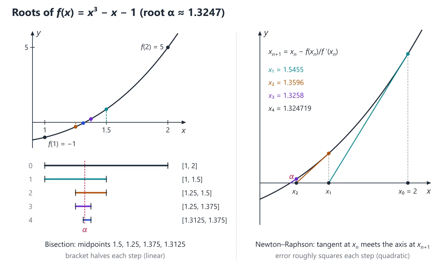
Example 1: f(x) = x3 − x − 1 on [1, 2], where f(1) = −1 and f(2) = 5.
Midpoints 1.5 (f = 0.875), 1.25 (f = −0.297), 1.375 (f = 0.225), 1.3125 (f = −0.052); the root lies in [1.3125, 1.375].
7. Regula-Falsi (False Position) Method
Replace the curve by the chord through (a, f(a)) and (b, f(b)): c = (a f(b) − b f(a))/(f(b) − f(a)); keep the sub-interval where the sign changes.
It always converges for continuous f with a sign change; the order is linear because one end point often stays fixed.
Idea: if f is convex on [a, b], every chord lies above the curve, so every new point c falls on the same side of the root and the far end point never moves; the bracket shrinks from one side only, which is why the order stays 1.
Example 2: x3 − x − 1 on [1, 2]: c1 = (1 · 5 − 2 · (−1))/6 = 7/6 ≈ 1.1667 and f(c1) ≈ −0.5787 < 0.
So the next interval is [1.1667, 2] and c2 = (1.1667 · 5 + 2 · 0.5787)/5.5787 ≈ 1.2531.
Secant method (no bracketing): xn+1 = xn − f(xn)(xn − xn−1)/(f(xn) − f(xn−1)), order (1 + √5)/2 ≈ 1.618 near a simple root.
Idea: the secant method is Newton's method with f′(xn) replaced by the slope of the chord through the last two iterates. Its error obeys en+1 ≈ Cenen−1, and trying en+1 ~ enp gives p2 = p + 1, whose positive root is the golden ratio 1.618.
8. Newton-Raphson Method
Formula: xn+1 = xn − f(xn)/f′(xn), the x-intercept of the tangent at xn (first-order Taylor expansion).
Idea: near a simple root the curve is almost straight, so the tangent at xn cuts the axis very close to the root (see the figure above). The tangent can mislead when the curve bends sharply or is nearly flat, which is what the failure cases in Section 13 describe.
Convergence: if f″ is continuous near a simple root α (f′(α) ≠ 0) and x0 is close enough to α, the iterates converge quadratically with en+1 ≈ [f″(α)/(2f′(α))]en2.
Sufficient condition: if f(a)f(b) < 0, f′ and f″ are non-zero with constant sign on [a, b], and x0 ∈ [a, b] satisfies f(x0)f″(x0) > 0, the iterates converge monotonically to the root.
At a root of multiplicity m convergence is only linear; xn+1 = xn − m f(xn)/f′(xn) restores quadratic convergence.
Why it works: if f = (x − α)mg with g(α) ≠ 0, then f/f′ = (x − α)g/(mg + (x − α)g′) ≈ (x − α)/m, so the Newton function φ = x − f/f′ has φ′(α) = 1 − 1/m ≠ 0 (linear, ratio (m − 1)/m); with the factor m, φ′(α) = 0 again.
Example 3: x3 − x − 1 = 0 with x0 = 1.5: xn+1 = xn − (xn3 − xn − 1)/(3xn2 − 1).
x1 = 1.347826, x2 = 1.325200, x3 = 1.324718; the root is 1.3247 to four decimals.
Square root: f(x) = x2 − N gives xn+1 = (xn + N/xn)/2; for N = 2 and x0 = 1: 1.5, 1.416667, 1.414216.
Other standard iterations: reciprocal 1/N without division, xn+1 = xn(2 − Nxn); k-th root, xn+1 = ((k − 1)xn + N/xnk−1)/k.
9. Derivation: Newton-Raphson and Regula-Falsi Formulae
Newton's formula: by Taylor's theorem 0 = f(α) = f(xn) + (α − xn)f′(xn) + (1/2)(α − xn)2f″(η) for some η between xn and α.
Dropping the quadratic term and solving for α gives the next approximation xn+1 = xn − f(xn)/f′(xn).
Quadratic convergence: keeping the term and dividing by f′(xn): α − xn + f(xn)/f′(xn) = −f″(η)(α − xn)2/(2f′(xn)), i.e. α − xn+1 = −f″(η)en2/(2f′(xn)).
Hence en+1 = [f″(η)/(2f′(xn))]en2, and as xn → α, en+1/en2 → f″(α)/(2f′(α)): order 2. For x3 − x − 1 this constant is 6α/(2(3α2 − 1)) ≈ 0.93, matching the errors of Example 3.
Regula-falsi formula: the chord through (a, f(a)) and (b, f(b)) is y − f(a) = [(f(b) − f(a))/(b − a)](x − a); putting y = 0 gives x = a − f(a)(b − a)/(f(b) − f(a)) = (af(b) − bf(a))/(f(b) − f(a)).
Iterations without division: for 1/N take f(x) = 1/x − N, f′(x) = −1/x2; then x − f/f′ = x + x2(1/x − N) = x(2 − Nx), which uses only multiplication.
10. Choosing the Method
If the question names a method → use it, even if another is faster, and say why it applies (sign change, f′ ≠ 0, |φ′| < 1).
If only a bracket is known and f′ is awkward → bisection (guaranteed, with the number of steps known in advance) or regula-falsi.
If f′ is easy to compute and a good starting value is available → Newton-Raphson, starting at the end where f(x0)f″(x0) > 0.
If f′ is unavailable or expensive → secant method from two nearby values.
If the equation rearranges as x = φ(x) → fixed-point iteration, choosing the rearrangement with the smallest |φ′| near the root.
If f and f′ are both small near the root (a multiple root) → modified Newton with the factor m.
11. Common Mistakes
A divergent rearrangement: for x3 − x − 1 = 0, x = x3 − 1 has φ′ = 3x2 ≈ 5.3 at the root and diverges; x = (x + 1)1/3 has φ′ ≈ 0.19 and converges.
Stopping on |f(xn)| alone: a flat function can be tiny far from its root; use the change |xn+1 − xn| as the main test.
Rounding too early: carry at least two more decimals than the answer needs, then round once at the end.
Replacing the wrong end point in bisection or regula-falsi: keep the end where f has the opposite sign to f(c).
Bisection step count: using log10 without dividing by log10 2, or not rounding n up to the next integer.
Starting Newton near a turning point: a tiny f′(x0) throws x1 far away; tabulate f first and start close to the root.
Link: the intermediate and mean value theorems come from Real Analysis, and the condition |φ′| ≤ k < 1 is the contraction mapping principle in one dimension.
Link: fixed-point iteration x = φ(x) is the one-variable model of the Jacobi and Gauss-Seidel methods x = Tx + c of the next topic, where |φ′| < 1 becomes 'spectral radius of T less than 1'.
12. Worked Examples
Example 4: How many bisection steps guarantee the root of x3 + x − 1 = 0 in [0, 1] to within 10−4? Carry out the first three steps.
f(0) = −1 and f(1) = 1, so a root lies in (0, 1); after n steps the error is at most 1/2n.
1/2n ≤ 10−4 needs 2n ≥ 104, i.e. n ≥ 4 log2 10 ≈ 13.29, so 14 steps suffice.
f(0.5) = −0.375 gives [0.5, 1]; f(0.75) = 0.171875 gives [0.5, 0.75]; f(0.625) = −0.130859 gives [0.625, 0.75]. (The root is 0.682328.)
Example 5: Find the root of x log10 x = 1.2 by the Newton-Raphson method, correct to four decimal places.
f(x) = x log10 x − 1.2, f′(x) = log10 x + log10 e = log10 x + 0.434294; f(2) = −0.598 and f(3) = 0.231, so the root lies in (2, 3).
x0 = 2.5: f(2.5) = −0.205150, f′(2.5) = 0.832234, so x1 = 2.5 + 0.246505 = 2.746505.
x2 = 2.740649, x3 = 2.740646; the root is 2.7406.
Example 6: Find the positive root of x3 + x2 − 1 = 0 by fixed-point iteration, choosing a convergent form.
f(0) = −1, f(1) = 1, so the root lies in (0, 1). Write x2(x + 1) = 1, i.e. x = φ(x) = 1/√(1 + x).
φ′(x) = −1/(2(1 + x)3/2), so |φ′(x)| ≤ 1/2 < 1 on [0, 1], and φ maps [0, 1] into itself: the iteration converges for every x0 in [0, 1].
x0 = 0.75: x1 = 0.755929, x2 = 0.754652, x3 = 0.754926, x4 = 0.754867, x5 = 0.754880; the root is 0.7549.
Example 7: Show that Newton's iteration for √N (N > 0) is xn+1 = (xn + N/xn)/2 and that en+1 = en2/(2xn), where en = xn − √N; deduce quadratic convergence for every x0 > 0.
f(x) = x2 − N, f′(x) = 2x: xn+1 = xn − (xn2 − N)/(2xn) = (xn + N/xn)/2.
xn+1 − √N = (xn2 − 2xn√N + N)/(2xn) = (xn − √N)2/(2xn), i.e. en+1 = en2/(2xn).
Hence en ≥ 0 for n ≥ 1; since 0 ≤ en ≤ xn, en+1 ≤ en/2, so xn decreases to √N, and en+1/en2 → 1/(2√N): the convergence is quadratic.
Example 8: Apply the secant method to x3 − 2x − 5 = 0 with x0 = 2, x1 = 3.
f(2) = −1, f(3) = 16: x2 = 3 − 16(3 − 2)/(16 + 1) = 2.058824, with f(x2) = −0.3908.
x3 = 2.081264 (f = −0.1472), x4 = 2.094824 (f = 0.0030), x5 = 2.094549; the root is 2.0946, reached much faster than by regula-falsi from the same bracket.
13. Locating Roots, Stopping Rules and Failure Cases
Tabulation: evaluate f at a few convenient points; each sign change brackets a root, giving starting values for bisection or regula-falsi and a good x0 for Newton's method (choose the end where f(x0)f″(x0) > 0).
Stopping rule: for 'correct to k decimal places' iterate until two successive iterates agree to k decimals, i.e. |xn+1 − xn| < 0.5 × 10−k, and then round; for 'k significant figures' apply the same test to the relative change.
Regula-falsi behaviour: if f″ keeps one sign on [a, b], one end point stays fixed and the error falls by a roughly constant factor each step (linear convergence); the secant method drops the bracket and gains order 1.618.
Algorithm (regula-falsi): read a, b, ε with f(a)f(b) < 0; repeat: c = (af(b) − bf(a))/(f(b) − f(a)); if f(a)f(c) < 0 then b = c else a = c; until two successive c differ by less than ε; print c.
When Newton's method fails: f′(xn) = 0 or very small (horizontal tangent); cycling, e.g. f(x) = x3 − 2x + 2 with x0 = 0 gives 0, 1, 0, 1, ...; divergence, e.g. f(x) = x1/3 gives xn+1 = −2xn; a start near a turning point jumping to another root; and only linear convergence at a multiple root.
14. Past UPSC Questions Solved
Example 9 (UPSC 2021, 10 marks): Find a positive root of the equation 3x = 1 + cos x by a numerical technique using initial values 0, π/2; and further improve the result using Newton-Raphson method correct to 8 significant figures.
f(x) = 3x − 1 − cos x is continuous, f(0) = −2 < 0 and f(π/2) = 3π/2 − 1 = 3.712389 > 0, so a root lies in (0, π/2); since f′(x) = 3 + sin x > 0, it is the only real root.
Regula-falsi with a = 0, b = π/2: c1 = (π/2)(2)/5.712389 = 0.549961 (f = −0.202661, so a = c1), c2 = 0.602804 (f = −0.015336), c3 = 0.606787 (f = −0.001125), c4 = 0.607079 (f = −0.000082).
Newton-Raphson xn+1 = xn − (3xn − 1 − cos xn)/(3 + sin xn) from x0 = 0.607079: f(x0) = −0.0000809, f′(x0) = 3.570471, so x1 = 0.60710165.
x2 = 0.60710165 again: the quadratic convergence roughly doubles the number of correct digits at each step.
Answer: x = 0.60710165 (8 significant figures).
Example 10 (UPSC 2023, 15 marks): Compute a root of the equation log10(2x + 1) − x2 + 3 = 0, in the interval [0, 3], by Regula-Falsi method, correct to 6 decimal places.
Let f(x) = log10(2x + 1) − x2 + 3: f(0) = 3, f(1) = 2.477121, f(2) = −0.301030, f(3) = −5.154902, so the root in [0, 3] lies in (1, 2); take a = 1, b = 2 (starting from [0, 3] also converges, only more slowly).
x1 = (1 · f(2) − 2 · f(1))/(f(2) − f(1)) = (−0.301030 − 4.954243)/(−2.778151) = 1.891644, with f(x1) = 0.101410 > 0, so the root lies in (1.891644, 2).
x2 = 1.918948 (f = 0.002294), x3 = 1.919561 (f = 0.0000511), x4 = 1.919575 (f = 0.0000011), x5 = 1.919575 (f ≈ 2.5 × 10⁻⁸).
The end b = 2 stays fixed throughout (f is concave on [1, 2]), which is the typical one-sided, linear convergence of regula-falsi.
Answer: x = 1.919575 (to 6 decimal places).
Example 11 (UPSC 2026, 10 marks): By using the Newton-Raphson iterative formula, establish the formula xi+1 = (1/3)(2xi + N/xi2) to find the cube root of N. Use this formula, if established, to find the cube root of 63 correct to four decimal places with the initial approximation 3·9.
f(x) = x3 − N, f′(x) = 3x2: xi+1 = xi − (xi3 − N)/(3xi2) = (2xi3 + N)/(3xi2) = (1/3)(2xi + N/xi2), which establishes the formula.
N = 63, x0 = 3.9: x1 = (1/3)(7.8 + 63/15.21) = (1/3)(7.8 + 4.142012) = 3.980671.
x2 = (1/3)(7.961341 + 63/15.845741) = (1/3)(7.961341 + 3.975833) = 3.979058, and x3 = 3.979057, which agrees with x2 to four decimals.
Answer: ∛63 = 3.9791 (to four decimal places).
15. Practice Exercises
Exercise 1 (basic): Show that x3 + 2x − 2 = 0 has a root in (0, 1) and carry out two bisection steps.
Answer: f(0) = −2, f(1) = 1; f(0.5) = −0.875 gives [0.5, 1]; f(0.75) = −0.078125 gives [0.75, 1] (the root is 0.770917).
Exercise 2 (basic): Use Newton's iteration xn+1 = xn(2 − Nxn) to compute 1/7 from x0 = 0.1 (three steps).
Answer: 0.13, 0.1417, 0.142848; 1/7 = 0.142857.
Exercise 3 (basic): How many bisection steps on [1, 2] guarantee an error at most 0.5 × 10⁻⁶ (using the bracket length as the error bound)?
Answer: 2−n ≤ 0.5 × 10⁻⁶ needs n ≥ 20.93, so 21 steps.
Exercise 4 (standard): Find the positive root of x4 − x − 10 = 0 by Newton-Raphson, starting from x0 = 2, correct to six decimals.
Answer: x1 = 1.870968, x2 = 1.855781, x3 = 1.855585, x4 = 1.855585.
Exercise 5 (standard): Apply two steps of regula-falsi to ex − 3x = 0 on [0, 1].
Answer: c1 = 0.780203 (f = −0.158694), new bracket [0, 0.780203]; c2 = 0.673347 (the root is 0.619061).
Exercise 6 (standard): Show that x = (cos x + 3)/2 converges from any x0, and find the root of 2x − cos x − 3 = 0 to four decimals.
Answer: |φ′(x)| = |sin x|/2 ≤ 1/2 for all x; from x0 = 1.5 the iterates settle at 1.5236.
Exercise 7 (standard): Apply the secant method to x2 − 5 = 0 with x0 = 2, x1 = 3 (three new iterates).
Answer: x2 = 2.2, x3 = 2.230769, x4 = 2.236111; √5 = 2.236068.
Exercise 8 (UPSC level): f(x) = (x − 1)2(x + 2) has a double root at 1. Starting from x0 = 2, compare two steps of Newton's method with two steps of xn+1 = xn − 2f(xn)/f′(xn).
Answer: f′ = 3(x − 1)(x + 1); Newton gives 1.555556, 1.297907 (errors roughly halve: linear); the modified rule gives 1.111111, 1.001949 (errors roughly squared: quadratic).
Exercise 9 (UPSC level): Find the smallest positive non-zero root of tan x = x to four decimals by Newton's method, and explain the choice of x0.
Answer: the root lies in (π, 3π/2); f = tan x − x, f′ = tan2x; start at 4.5, safely left of the pole 3π/2 ≈ 4.712: x1 = 4.493614, x2 = 4.493409, so x = 4.4934.
Exercise 10 (UPSC level): Show that xn+1 = xn(xn2 + 3N)/(3xn2 + N) converges to √N with order 3.
Answer: x(x2 + 3N) − √N(3x2 + N) = (x − √N)3, so en+1 = en3/(3xn2 + N) ≈ en3/(4N).
| Method | Order | Needs | Convergence guaranteed? |
|---|---|---|---|
| Bisection | 1 (error halves) | Sign change | Yes |
| Regula-Falsi | 1 | Sign change | Yes |
| Secant | ≈ 1.618 | Two starting values | No |
| Newton-Raphson | 2 (simple root) | f′ and a good x0 | No (locally yes) |
Mains points
- Typical questions ask for a root correct to three or four decimals by a named method; tabulate n, xn, f(xn) and stop with a clear criterion.
- Derive the Newton-Raphson formula geometrically or from Taylor's series and prove its quadratic convergence; this is a standard theory part.
- Iterative formulas for √N, 1/N or N1/k by Newton's method are frequently asked as 10-mark questions.
- For bisection, the number of iterations needed for a given accuracy is a quick, commonly asked computation.
- Common mistake: using degrees instead of radians for transcendental equations like x − cos x = 0, or stopping without checking the sign of f at the final value.
Did you know?
- The square-root iteration xn+1 = (xn + N/xn)/2 was used by Babylonian scribes about 4000 years ago, long before Newton; each step roughly doubles the number of correct digits.
Systems of Linear Equations: Direct and Iterative Methods
Direct methods give the solution of Ax = b in a finite number of operations: Gaussian elimination reduces A to upper triangular form and back-substitutes, while Gauss-Jordan reduces A to the identity. The Gauss-Seidel iterative method updates one unknown at a time using the newest values and converges for any starting vector when A is strictly diagonally dominant.
1. Understanding Gaussian Elimination and Back Substitution
Why we need it: Cramer's rule needs n + 1 determinants and becomes hopeless beyond n = 3 or 4. Elimination solves Ax = b for any n with about n3/3 multiplications, by a procedure simple enough to program.
In words: the pivot akk is the entry used to clear column k below the diagonal; the multiplier of row i is mik = aik/akk, and Ri → Ri − mikRk removes the k-th unknown from equation i.
Such row operations replace an equation by an equivalent one, so the solution never changes. When every column is cleared the matrix is upper triangular, and back substitution solves from the last equation upwards.
First example, slowly: solve 2x + y − z = 8, −3x − y + 2z = −11, −2x + y + 2z = −3.
Step 1: write the augmented rows (2, 1, −1 | 8), (−3, −1, 2 | −11), (−2, 1, 2 | −3); the first pivot is 2.
Step 2: multipliers m21 = −3/2 and m31 = −1; R2 + (3/2)R1 = (0, 1/2, 1/2 | 1) and R3 + R1 = (0, 2, 1 | 5).
Step 3: the second pivot is 1/2 and m32 = 2/(1/2) = 4; R3 − 4R2 = (0, 0, −1 | 1). The matrix is now upper triangular.
Step 4: back substitution: the last row gives −z = 1, so z = −1.
Step 5: the second row gives y/2 + z/2 = 1, so y = 2 − z = 3.
Step 6: the first row gives 2x + 3 − (−1) = 8, so x = 2.
Step 7: check in the original third equation: −4 + 3 − 2 = −3. The pivots are 2, 1/2, −1, so det A = 2 × (1/2) × (−1) = −1.
Non-example: for y + z = 2, x + y = 1, x + z = 3 the first pivot a11 is 0, so no multiplier can be formed and the elimination cannot start as written. The matrix is not singular (its determinant is −2); the remedy is a row interchange. The condition that fails is a non-zero pivot.
Building up: clearing column k touches about (n − k)2 entries, so the total work is about n3/3, while back substitution costs only about n2/2.
Each row operation is multiplication by a unit lower triangular matrix, so elimination is the factorisation A = LU ('Derivation: Elimination Is a Factorisation' below), and the product of the pivots is det A.
Where it is used: 3 × 3 systems in 10–15 mark questions, rank and consistency in Linear Algebra, and the algorithm with partial pivoting in the last topic.
2. Understanding Partial Pivoting and Ill-Conditioning
Why we need it: a computer keeps only a fixed number of digits. A small pivot creates a huge multiplier that swamps the other entries in rounding, and the computed answer can be completely wrong even though every step was 'correct'.
In words: partial pivoting means: before clearing column k, look at the entries of column k on and below the diagonal, and swap rows so that the one of largest absolute value becomes the pivot. Then every multiplier has |mik| ≤ 1.
Ill-conditioning is a different problem: it belongs to the system itself, not to the method. If tiny changes in the data cause large changes in the solution, no method can give more accuracy than the data allow; the condition number ‖A‖‖A−1‖ measures this sensitivity.
First example, slowly: solve 0.003x + 59.14y = 59.17, 5.291x − 6.130y = 46.78 (exact solution x = 10, y = 1) in 4-significant-digit arithmetic, without and with pivoting.
Step 1: without pivoting the multiplier is m = 5.291/0.003 = 1764 (rounded).
Step 2: the new second row: −6.130 − 1764 × 59.14 rounds to −104300, and 46.78 − 1764 × 59.17 rounds to −104400; the small numbers −6.130 and 46.78 are lost in the rounding.
Step 3: so y = −104400/(−104300) = 1.001, and x = (59.17 − 59.14 × 1.001)/0.003 = (59.17 − 59.20)/0.003 = −10.00. The tiny error in y is divided by the tiny pivot 0.003 and becomes a disaster in x.
Step 4: with pivoting, the largest entry of column 1 is 5.291, so swap the rows; now m = 0.003/5.291 = 0.000567.
Step 5: the new second row: 59.14 + 0.000567 × 6.130 rounds to 59.14, and 59.17 − 0.000567 × 46.78 rounds to 59.14, so y = 1.000.
Step 6: back substitution: x = (46.78 + 6.130 × 1.000)/5.291 = 52.91/5.291 = 10.00, correct to the digits carried.
Step 7: notice that the system was harmless; only the order of the rows caused the failure, and pivoting removed it.
Non-example: x + 2y = 3, 1.001x + 2y = 3.001 has solution (1, 1), but changing 3.001 to 3.002 gives (2, 0.5). Pivoting cannot help here, because the two lines are almost parallel and the solution itself is sensitive (the condition number is about 6000). The condition that fails is good conditioning, which no algorithm can supply.
Building up: pivoting keeps |mik| ≤ 1, which limits the growth of rounding errors; the relative error of the answer is then roughly the condition number times the relative error of the data, ‖δx‖/‖x‖ ≤ ‖A‖‖A−1‖ ‖δb‖/‖b‖.
Where it is used: 'solve by Gaussian elimination with partial pivoting' questions, the remark on ill-conditioning that examiners reward, and every library routine for linear systems.
3. Understanding LU Decomposition
Why we need it: in practice the same matrix A is used with many right-hand sides b (different loads on one structure, different time steps). Repeating the elimination for each b wastes the n3/3 work; factorising A once avoids that.
In words: A = LU with L unit lower triangular (1s on the diagonal, the multipliers below it) and U upper triangular (the result of elimination). Then Ax = b splits into two triangular systems: Ly = b by forward substitution and Ux = y by back substitution.
Each triangular solve costs about n2/2 operations, so after the factorisation every new b is cheap.
First example, slowly: factorise A = [[2, 1, 1], [4, 3, 3], [8, 7, 9]] and solve Ax = (4, 10, 24).
Step 1: column 1: multipliers l21 = 4/2 = 2 and l31 = 8/2 = 4; R2 − 2R1 = (0, 1, 1) and R3 − 4R1 = (0, 3, 5).
Step 2: column 2: l32 = 3/1 = 3; (0, 3, 5) − 3(0, 1, 1) = (0, 0, 2).
Step 3: so U = [[2, 1, 1], [0, 1, 1], [0, 0, 2]] and L = [[1, 0, 0], [2, 1, 0], [4, 3, 1]]; multiplying back, row 3 of LU is 4(2, 1, 1) + 3(0, 1, 1) + (0, 0, 2) = (8, 7, 9).
Step 4: forward substitution Ly = b: y1 = 4, y2 = 10 − 2(4) = 2, y3 = 24 − 4(4) − 3(2) = 2.
Step 5: back substitution Ux = y: 2x3 = 2 gives x3 = 1; x2 + x3 = 2 gives x2 = 1; 2x1 + 1 + 1 = 4 gives x1 = 1.
Step 6: check: A(1, 1, 1) = (4, 10, 24). For another right side only Steps 4 and 5 need to be repeated.
Non-example: A = [[0, 1], [1, 1]] is invertible but has no factorisation A = LU with unit lower L: it would need u11 = 0 and then l21u11 = 1, which is impossible. The condition that fails is 'leading principal minors non-zero'; with a row interchange PA = LU always exists.
Building up: the Doolittle formulas compute the same L and U directly, row by row ('LU Decomposition and Practical Points' below); Crout's variant puts the 1s on the diagonal of U, and for a symmetric positive definite A the Cholesky form A = LLT halves the work.
Where it is used: 'solve by LU decomposition' questions, determinants (det A = u11u22 ··· unn), and inverses computed column by column from LU.
4. Understanding Jacobi and Gauss-Seidel Iteration
Why we need it: the systems produced by discretising Laplace's equation can have millions of unknowns, but each equation involves only a few of them. Elimination would fill in the zeros; iteration works with the equations as they are and needs only about n2 (or less) work per sweep.
In words: solve equation i for its own unknown xi, guess all the unknowns, and use the equations to improve the guess. Jacobi uses only the old values on the right; Gauss-Seidel uses each new value as soon as it has been computed.
The error obeys e(k+1) = Te(k) for a fixed iteration matrix T, so the method converges for every start exactly when the spectral radius ρ(T) (largest |eigenvalue|) is less than 1. Strict diagonal dominance is an easy sufficient test.
First example, slowly: solve 4x + y = 6, x + 3y = 7 (exact solution (1, 2)) by Jacobi and by Gauss-Seidel from (0, 0).
Step 1: the system is strictly diagonally dominant (4 > 1, 3 > 1), so both methods converge. Write x = (6 − y)/4 and y = (7 − x)/3.
Step 2: Jacobi, both updates from the old pair: (1.5, 2.3333), (0.9167, 1.8333), (1.0417, 2.0278), (0.9931, 1.9861).
Step 3: Gauss-Seidel, the new x used at once in y: x = 1.5, then y = (7 − 1.5)/3 = 1.8333.
Step 4: continuing: (1.0417, 1.9861), (1.0035, 1.9988), (1.0003, 1.9999).
Step 5: compare the rates: the Jacobi matrix [[0, −1/4], [−1/3, 0]] has eigenvalues ±√(1/12) ≈ ±0.289, while the Gauss-Seidel matrix has spectral radius 1/12 ≈ 0.083, the square.
Step 6: so each Gauss-Seidel sweep does the work of about two Jacobi sweeps, as the numbers show.
Non-example: x + 3y = 4, 2x + y = 3 also has solution (1, 1), but Jacobi from (0, 0) gives (4, 3), (−5, −5), (19, 13), (−35, −35): it diverges, because the iteration matrix has eigenvalues ±√6 and ρ ≈ 2.45 > 1. Interchanging the equations gives a dominant system that converges. The condition that fails is ρ(T) < 1.
Building up: writing A = L + D + U, Jacobi is x(k+1) = −D−1(L + U)x(k) + D−1b and Gauss-Seidel is (D + L)x(k+1) = b − Ux(k); dominance makes ‖T‖∞ < 1 for Jacobi ('Why it works' under Gauss-Seidel below).
Dominance is sufficient, not necessary, and the two methods can disagree: there are matrices for which Jacobi converges and Gauss-Seidel diverges (Exercise 9 below).
Where it is used: 'solve by Gauss-Seidel after checking that the method applies' questions (UPSC 2019, 2021), and the finite-difference solution of Laplace's equation in the PDE chapter.
5. Gaussian Elimination
Form the augmented matrix [A | b]. Forward elimination: for k = 1, ..., n − 1 and each i > k, Ri → Ri − (aik/akk)Rk, making A upper triangular.
Idea: each row operation replaces an equation by an equivalent one, so the solution never changes; elimination is the school method of removing one unknown at a time, organised column by column so that it can be programmed. akk is the pivot and aik/akk the multiplier.
Back substitution: xn = bn/ann, then xi = (bi − ∑j > i aijxj)/aii for i = n − 1, ..., 1.
Idea: a triangular system is easy because the last equation has a single unknown, and each earlier equation brings in exactly one new unknown; this step costs only about n2/2 operations.
Partial pivoting: before eliminating column k, interchange rows so that the entry of largest absolute value in column k (on or below the diagonal) becomes the pivot; this avoids zero pivots and limits the growth of round-off error.
Idea: a tiny pivot gives a huge multiplier, which swamps the other entries in rounding. In 3-digit arithmetic, 0.0001x + y = 1, x + y = 2 without pivoting gives −1.00 × 10⁴y = −1.00 × 10⁴, so y = 1.00 and then x = 0, although the true solution is x = 1.0001, y = 0.9999. Interchanging the rows first gives y = 1.00, x = 1.00, correct to three figures.
Cost: about n3/3 multiplications.
Why it works: clearing column k changes (n − k) rows of about (n − k) entries each, so the work is ∑(n − k)2 ≈ n3/3; doubling n multiplies the work by about 8.
Example 1: x + y + z = 6, 2x + 3y + z = 11, x + 2y + 3z = 14.
R2 − 2R1: y − z = −1; R3 − R1: y + 2z = 8; then R3 − R2: 3z = 9.
Back substitution: z = 3, y = −1 + 3 = 2, x = 6 − 2 − 3 = 1.
6. Gauss-Jordan Method
Eliminate each pivot variable from all other rows, above as well as below, and scale each pivot to 1, so that [A | b] becomes [I | x] and the solution is read off directly.
Cost: about n3/2 multiplications, more than Gaussian elimination; applied to [A | I] it produces [I | A−1], the standard way to invert a matrix.
Idea: for one right-hand side Gaussian elimination with back substitution is cheaper; Gauss-Jordan pays off when the whole inverse is wanted, because the n columns of I are carried along at once.
Example 2: from the triangular rows (1, 1, 1 | 6), (0, 1, −1 | −1), (0, 0, 3 | 9): R3/3 gives (0, 0, 1 | 3); R2 + R3 gives (0, 1, 0 | 2); R1 − R2 − R3 gives (1, 0, 0 | 1).
So [I | x] shows x = 1, y = 2, z = 3.
Direct methods give the exact solution in finitely many steps, apart from round-off error.
Ill-conditioning: if small changes in A or b cause large changes in x, the system is ill-conditioned; the condition number ‖A‖‖A−1‖ measures this.
Idea: geometrically, the equations are nearly parallel lines, so a small shift moves their intersection a long way. x + y = 2, x + 1.0001y = 2.0001 has solution (1, 1), but changing 2.0001 to 2.0002 gives (0, 2). In general ‖δx‖/‖x‖ ≤ ‖A‖‖A−1‖ · ‖δb‖/‖b‖, and no method can beat the condition number.
7. Gauss-Seidel Method
Solve the i-th equation for xi: xi = (bi − ∑j≠i aijxj)/aii.
Idea: guess and improve: each equation is used to correct 'its own' unknown, which works well when that unknown dominates the equation (a large aii), because errors in the other unknowns are then divided by a large number.
Gauss-Seidel: xi(k+1) = (bi − ∑j < i aijxj(k+1) − ∑j > i aijxj(k))/aii, using each new value as soon as it is available.
Jacobi method: uses only the old values x(k) on the right; when both converge, Gauss-Seidel is usually faster (about twice as fast for many common matrices).
Sufficient condition: if A is strictly diagonally dominant, |aii| > ∑j≠i|aij| for every i, both Jacobi and Gauss-Seidel converge for any starting vector; Gauss-Seidel also converges when A is symmetric positive definite.
Why it works (Jacobi): the error e(k) = x(k) − x satisfies e(k+1) = Te(k) with T = −D−1(L + U); row i of T has absolute sum ∑j≠i|aij|/|aii| < 1, so ‖T‖∞ = q < 1 and ‖e(k)‖∞ ≤ qk‖e(0)‖∞ → 0. Dominance is sufficient, not necessary.
Necessary and sufficient condition: writing A = L + D + U, Gauss-Seidel is x(k+1) = −(D + L)−1Ux(k) + (D + L)−1b, which converges for every start if and only if the spectral radius of (D + L)−1U is less than 1.
Why it works: from Ax = b, (D + L)x = b − Ux; subtracting this from the iteration (D + L)x(k+1) = b − Ux(k) gives e(k+1) = Ge(k) with G = −(D + L)−1U, so e(k) = Gke(0), and Gk → 0 exactly when every eigenvalue of G has modulus less than 1.
Rearrange the equations to make the system diagonally dominant before iterating, and stop when successive iterates agree to the required accuracy.
Example 3: 10x + y + z = 12, x + 10y + z = 12, x + y + 10z = 12, starting from (0, 0, 0).
Iteration 1: x = 1.2, y = (12 − 1.2)/10 = 1.08, z = (12 − 1.2 − 1.08)/10 = 0.972.
Iteration 2: x = 0.9948, y = 1.0033, z = 1.0002.
Iteration 3: x = 0.99965, y = 1.00002, z = 1.00003; the exact solution is (1, 1, 1).
8. Derivation: Elimination Is a Factorisation
The step Ri → Ri − mikRk is multiplication on the left by Eik = I − mikeiekT, a unit lower triangular matrix whose inverse is I + mikeiekT.
Forward elimination is therefore E A = U with E a product of such matrices, so A = E−1U = LU, where L is unit lower triangular with the multipliers mik in place (Section 12 computes it directly by Doolittle's formulas).
Consequences: det A = (product of the pivots) × (−1)number of row interchanges, and a zero pivot that no interchange can remove means A is singular.
Check on Example 1: the pivots are 1, 1, 3 with no interchange, so det A = 3; directly, det [[1, 1, 1], [2, 3, 1], [1, 2, 3]] = 1(9 − 2) − 1(6 − 1) + 1(4 − 3) = 3.
Why Gauss-Seidel is usually faster than Jacobi: it uses each improved value at once, so within one sweep the later equations already see part of the correction; for many common matrices (tridiagonal ones, for example) its spectral radius is the square of Jacobi's, which halves the number of iterations.
9. Choosing the Method
If the system is small and dense and an exact answer is wanted → Gaussian elimination with partial pivoting.
If the inverse is wanted → Gauss-Jordan on [A | I]; if many right-hand sides share one A → factorise A = LU once and do two triangular solves for each b.
If the system is large, sparse and diagonally dominant → Gauss-Seidel (or Jacobi when the updates must be independent, as on parallel machines).
If the rows are not dominant as given → reorder the equations; if no order is dominant → check the spectral radius, or use a direct method.
If A is symmetric positive definite → Gauss-Seidel is guaranteed to converge, and the Cholesky factorisation A = LLT halves the work of LU.
10. Common Mistakes
Swapping rows of A but not of b: in the augmented matrix the right-hand entry moves with its row.
Pivoting along the row: partial pivoting chooses the largest |aik| in the current column on or below the diagonal, not the largest entry of the row.
Rounding early in hand work: keep fractions (5/3, 7/3, ...) until back substitution, as in Example 4; decimals rounded at each step can spoil the last digit.
Declaring a system singular at the first zero pivot without trying a row interchange; a first equation with no x1 term only needs its row swapped with a lower one.
Iterating without a convergence argument: state diagonal dominance (or rearrange to obtain it) before the first iteration, and stop on the stated accuracy, not after an arbitrary number of sweeps.
Mixing Doolittle and Crout: Doolittle puts 1s on the diagonal of L, Crout on the diagonal of U; decide first and keep to it.
Link: Gaussian elimination is the row reduction to echelon form used for rank, consistency and inverses in Linear Algebra; the convergence test 'spectral radius less than 1' is a statement about eigenvalues.
Link: Jacobi and Gauss-Seidel are fixed-point iteration (previous topic) for vectors, and they are the standard way to solve the large systems produced by finite-difference forms of Laplace's equation (PDE chapter).
11. Worked Examples
Example 4: Solve x + 2y + 3z = 14, 3x + y + 2z = 11, 2x + 3y + z = 11 by Gaussian elimination with partial pivoting.
Column 1: the largest pivot is 3, so interchange R1 and R2: (3, 1, 2 | 11), (1, 2, 3 | 14), (2, 3, 1 | 11).
R2 − (1/3)R1 = (0, 5/3, 7/3 | 31/3) and R3 − (2/3)R1 = (0, 7/3, −1/3 | 11/3).
Column 2: 7/3 > 5/3, so interchange these two rows; then (0, 5/3, 7/3 | 31/3) − (5/7)(0, 7/3, −1/3 | 11/3) = (0, 0, 18/7 | 54/7).
Back substitution: z = 3; (7/3)y − 1 = 11/3 gives y = 2; 3x + 2 + 6 = 11 gives x = 1.
Example 5: Find the inverse of A = [[2, 1, 1], [1, 2, 1], [1, 1, 2]] by the Gauss-Jordan method.
Start from [A | I]. Column 1 (R1/2, then R2 − R1, R3 − R1): (1, 1/2, 1/2 | 1/2, 0, 0), (0, 3/2, 1/2 | −1/2, 1, 0), (0, 1/2, 3/2 | −1/2, 0, 1).
Column 2 (R2 × 2/3, then clear above and below): (1, 0, 1/3 | 2/3, −1/3, 0), (0, 1, 1/3 | −1/3, 2/3, 0), (0, 0, 4/3 | −1/3, −1/3, 1).
Column 3 (R3 × 3/4, then clear): (1, 0, 0 | 3/4, −1/4, −1/4), (0, 1, 0 | −1/4, 3/4, −1/4), (0, 0, 1 | −1/4, −1/4, 3/4).
So A−1 = (1/4)[[3, −1, −1], [−1, 3, −1], [−1, −1, 3]]; check: row 1 of A times column 1 of A−1 is (6 − 1 − 1)/4 = 1, and row 1 times column 2 is (−2 + 3 − 1)/4 = 0.
Example 6: Solve 27x + 6y − z = 85, 6x + 15y + 2z = 72, x + y + 54z = 110 by the Jacobi and Gauss-Seidel methods from (0, 0, 0), and compare.
The matrix is strictly diagonally dominant (27 > 7, 15 > 8, 54 > 2), so both methods converge.
Jacobi: (3.1481, 4.8000, 2.0370), (2.1569, 3.2691, 1.8898), (2.4917, 3.6852, 1.9366), (2.4009, 3.5451, 1.9226), (2.4316, 3.5833, 1.9269).
Gauss-Seidel: (3.1481, 3.5407, 1.9132), (2.4322, 3.5720, 1.9258), (2.4257, 3.5729, 1.9260), (2.4255, 3.5730, 1.9260).
Solution x = 2.4255, y = 3.5730, z = 1.9260: Gauss-Seidel settles in four iterations, while Jacobi is still oscillating after five.
Example 7: Prove or disprove: the Gauss-Seidel method converges for every system with a non-singular coefficient matrix.
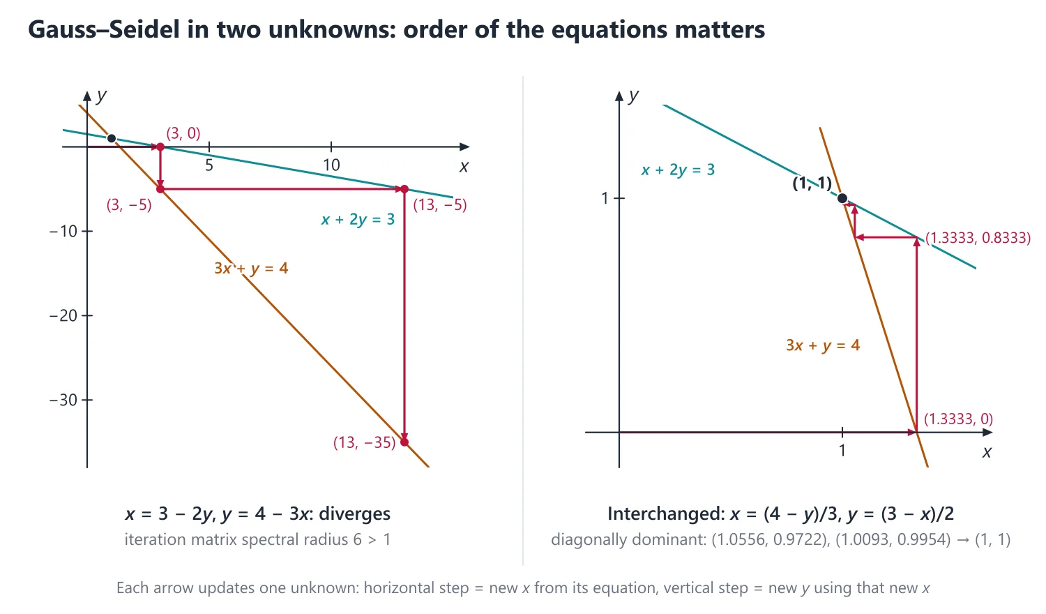
False. For x + 2y = 3, 3x + y = 4 (solution (1, 1)), the iteration x = 3 − 2y, y = 4 − 3x from (0, 0) gives (3, −5), (13, −35), (73, −215), which diverges.
Its iteration matrix −(D + L)−1U = [[0, −2], [0, 6]] has spectral radius 6 > 1.
Interchanging the equations gives the diagonally dominant system 3x + y = 4, x + 2y = 3; then x = (4 − y)/3, y = (3 − x)/2 gives (1.3333, 0.8333), (1.0556, 0.9722), (1.0093, 0.9954), (1.0015, 0.9992) → (1, 1).
12. LU Decomposition and Practical Points
LU decomposition: if all leading principal minors of A are non-zero, A = LU with L unit lower triangular and U upper triangular (Doolittle's method); Crout's method puts the 1s on the diagonal of U instead.
Doolittle formulas: u1j = a1j, li1 = ai1/u11; then row by row uij = aij − ∑k=1i−1 likukj (j ≥ i) and lij = (aij − ∑k=1j−1 likukj)/ujj (i > j).
Ax = b is then solved as Ly = b (forward substitution) and Ux = y (back substitution); L holds the multipliers of Gaussian elimination, so one factorisation serves many right-hand sides.
Example 8: Solve x + y + z = 1, 4x + 3y − z = 6, 3x + 5y + 3z = 4 by LU decomposition.
u11 = u12 = u13 = 1; l21 = 4, l31 = 3; u22 = 3 − 4 = −1, u23 = −1 − 4 = −5; l32 = (5 − 3)/(−1) = −2; u33 = 3 − 3 − (−2)(−5) = −10.
Ly = b: y1 = 1, y2 = 6 − 4 = 2, y3 = 4 − 3 + 2(2) = 5; Ux = y: −10z = 5, −y − 5z = 2, x + y + z = 1 give z = −1/2, y = 1/2, x = 1 (check: 3 + 5/2 − 3/2 = 4).
Main steps of Gauss-Jordan (theory part): (1) write [A | b] or [A | I]; (2) for k = 1 to n pick a non-zero (preferably the largest) pivot in column k, interchange rows if needed and divide the pivot row by the pivot; (3) subtract multiples of the pivot row from all other rows so column k becomes a unit vector; (4) read x or A−1 from the right block; a zero column below and at the pivot means A is singular.
Rearranging for Gauss-Seidel: for each unknown choose the equation in which its coefficient dominates the others, so that every row becomes strictly diagonally dominant; then convergence is guaranteed. Dominance is sufficient, not necessary: the real test is that the spectral radius of the iteration matrix is less than 1.
13. Past UPSC Questions Solved
Example 9 (UPSC 2021, 15 marks): Solve the system of equations 3x1 + 9x2 − 2x3 = 11, 4x1 + 2x2 + 13x3 = 24, 4x1 − 2x2 + x3 = −8 correct up to 4 significant figures by using Gauss-Seidel method after verifying whether the method is applicable in your transformed form of the system.
As written no row is diagonally dominant. Rearrange: the third equation for x1 (|4| > |−2| + |1|), the first for x2 (|9| > |3| + |−2|) and the second for x3 (|13| > |4| + |2|).
The system 4x1 − 2x2 + x3 = −8, 3x1 + 9x2 − 2x3 = 11, 4x1 + 2x2 + 13x3 = 24 is strictly diagonally dominant, so Gauss-Seidel is applicable and converges from any start.
Scheme: x1 = (−8 + 2x2 − x3)/4, x2 = (11 − 3x1 + 2x3)/9, x3 = (24 − 4x1 − 2x2)/13, starting from (0, 0, 0).
Iterates: (−2, 1.88889, 2.17094), (−1.59829, 2.23742, 1.99372), (−1.37972, 2.12518, 1.94373), (−1.42334, 2.12861, 1.95663), (−1.42485, 2.13198, 1.95657), (−1.42315, 2.13140, 1.95614), (−1.42333, 2.13136, 1.95620), (−1.42337, 2.13139, 1.95621).
Answer: x1 = −1.423, x2 = 2.131, x3 = 1.956 (4 significant figures); the exact solution is (−195/137, 292/137, 268/137).
Example 10 (UPSC 2019, 15 marks): Apply Gauss-Seidel iteration method to solve the following system of equations :
2x + y − 2z = 17,
3x + 20y − z = −18,
2x − 3y + 20z = 25, correct to three decimal places.
[As printed, the first coefficient is 2; textbooks often print 20x + y − 2z = 17, which is solved in the Solved Problems topic (answer (1, −1, 1)). The printed system is solved here.]
Scheme: x = (17 − y + 2z)/2, y = (−18 − 3x + z)/20, z = (25 − 2x + 3y)/20 from (0, 0, 0). Row 1 is not dominant (2 < 1 + 2), but the Gauss-Seidel iteration matrix has spectral radius about 0.074 < 1, so the method converges.
Iterates: (8.5, −2.175, 0.07375), (9.66125, −2.34550, −0.06795), (9.60480, −2.34412, −0.06210), (9.60996, −2.34460, −0.06269), (9.60961, −2.34458, −0.06265), (9.60964, −2.34458, −0.06265).
Answer: x = 9.610, y = −2.345, z = −0.063 (three decimals); exactly (3988/415, −973/415, −26/415), which satisfies all three equations.
14. Practice Exercises
Exercise 1 (basic): Solve the triangular system 2x + y + z = 6, 3y − z = 4, 2z = 4.
Answer: z = 2, y = (4 + 2)/3 = 2, x = (6 − 2 − 2)/2 = 1.
Exercise 2 (basic): Is [[5, 2, 1], [1, 4, 2], [2, 1, 6]] strictly diagonally dominant? What does that guarantee?
Answer: yes (5 > 3, 4 > 3, 6 > 3); Jacobi and Gauss-Seidel converge for every right side and every starting vector.
Exercise 3 (basic): Write the Jacobi formulas for 10x + y = 11, 2x + 10y = 12 and perform one iteration from (0, 0).
Answer: x = (11 − y)/10, y = (12 − 2x)/10; one step gives (1.1, 1.2) (the solution is (1, 1)).
Exercise 4 (standard): Solve x + y + z = 9, 2x − 3y + 4z = 13, 3x + 4y + 5z = 40 by Gaussian elimination.
Answer: R2 − 2R1: −5y + 2z = −5; R3 − 3R1: y + 2z = 13; then 12z = 60, so z = 5, y = 3, x = 1.
Exercise 5 (standard): Find the inverse of [[1, 2], [3, 4]] by the Gauss-Jordan method.
Answer: [[−2, 1], [3/2, −1/2]].
Exercise 6 (standard): Find the Doolittle factorisation of [[1, 1, 1], [2, 3, 1], [1, 2, 3]].
Answer: L = [[1, 0, 0], [2, 1, 0], [1, 1, 1]], U = [[1, 1, 1], [0, 1, −1], [0, 0, 3]] (det = 3).
Exercise 7 (standard): Perform three Gauss-Seidel iterations for 5x + y = 7, x + 4y = 6 from (0, 0) and compare with the exact solution.
Answer: (1.4, 1.15), (1.17, 1.2075), (1.1585, 1.210375); exact (22/19, 23/19) = (1.157895, 1.210526).
Exercise 8 (UPSC level): Solve 2x + 3y − z = 5, 4x + 4y − 3z = 3, −2x + 3y − z = 1 by Gaussian elimination with partial pivoting.
Answer: pivot 4 (row 2 first), then pivot 5 in column 2; the solution is x = 1, y = 2, z = 3.
Exercise 9 (UPSC level): For A = [[1, 2, −2], [1, 1, 1], [2, 2, 1]] show that the Jacobi method converges while the Gauss-Seidel method diverges.
Answer: the Jacobi matrix T satisfies T3 = 0 (all eigenvalues 0), so Jacobi reaches the solution in at most three steps; the Gauss-Seidel matrix has eigenvalues 0, 2, 2, so ρ = 2 > 1 and it diverges (for b = (1, 3, 5) the iterates from 0 grow without bound).
Exercise 10 (UPSC level): Compute the condition number ‖A‖∞‖A−1‖∞ of A = [[1, 2], [1.001, 2]] and interpret it.
Answer: A−1 = [[−1000, 1000], [500.5, −500]], ‖A‖∞ = 3.001, ‖A−1‖∞ = 2000, so the condition number is 6002: a relative change in b can be magnified up to about 6000 times in x.
| Feature | Gaussian elimination / Gauss-Jordan | Gauss-Seidel |
|---|---|---|
| Result | Exact apart from round-off, in finite steps | Approximation improved each iteration |
| Cost | About n3/3 (Gauss) or n3/2 (Gauss-Jordan) | About n2 per iteration |
| Condition for success | Non-singular A (pivoting for stability) | Convergence, e.g. strict diagonal dominance |
| Best suited to | Small dense systems, matrix inversion | Large sparse diagonally dominant systems |
| Form of the problem | Method | Watch out for |
|---|---|---|
| Small dense system | Gaussian elimination with partial pivoting | Swap b with its row |
| Inverse required | Gauss-Jordan on [A | I] | Verify one row of AA−1 = I |
| Same A, many b | LU decomposition | Leading minors non-zero (else pivot) |
| Large, sparse, diagonally dominant | Gauss-Seidel | Use new values at once |
| Not dominant | Reorder rows, or a direct method | Dominance is sufficient, not necessary |
| Symmetric positive definite | Cholesky or Gauss-Seidel | Check symmetry first |
Mains points
- A 3 × 3 system by Gaussian elimination with partial pivoting, or by Gauss-Jordan, is a common 10–15 mark question; show every row operation.
- For Gauss-Seidel, first check or arrange diagonal dominance and say so; then tabulate iterations to the stated accuracy.
- Questions may ask to find A−1 by Gauss-Jordan; carry [A | I] through to [I | A−1] and verify AA−1 = I for one row.
- Know the difference between Jacobi and Gauss-Seidel and the convergence conditions; short theory parts ask for them.
- Common mistake: in Gauss-Seidel, using old values for variables already updated in the same sweep (that is the Jacobi method).
Did you know?
- Elimination for linear systems appears in the Chinese text Nine Chapters on the Mathematical Art (around 200 BCE to 100 CE), almost two thousand years before Gauss.
Interpolation: Newton's Forward, Backward and Lagrange's Formulae
Interpolation finds the unique polynomial of degree ≤ n through n + 1 data points and uses it to estimate intermediate values. For equally spaced data, Newton's forward formula (near the start of the table) and backward formula (near the end) use finite differences. For unequally spaced data, Lagrange's formula writes the polynomial as ∑Li(x)yi. The error involves f(n+1)(ξ)/(n + 1)!.
1. Understanding the Difference Table
Why we need it: tables of values at equal steps (of a function, or of measurements) are the raw material of interpolation. Before choosing a formula we need to see how the values change from row to row, and the difference table shows this at a glance.
In words: with xi = x0 + ih, the first difference Δyi = yi+1 − yi is the change over one step; Δ2yi = Δyi+1 − Δyi is the change of the change, and so on. Each column of the table is formed by subtracting neighbours in the column to its left.
Differences behave like derivatives: for a polynomial of degree n the n-th differences are constant (n!anhn) and the higher ones are zero. So the table reveals the degree of the data.
First example, slowly: build the forward difference table of y = x3 − 2x for x = 0, 1, 2, 3, 4.
Step 1: the values are y = 0, −1, 4, 21, 56.
Step 2: first differences: −1 − 0 = −1, 4 − (−1) = 5, 21 − 4 = 17, 56 − 21 = 35.
Step 3: second differences: 6, 12, 18.
Step 4: third differences: 6, 6; fourth difference: 0.
Step 5: the third differences are constant, as they must be for a cubic: 3! × a3 × h3 = 6 × 1 × 1 = 6.
Step 6: read the table by diagonals: the top diagonal y0 = 0, Δy0 = −1, Δ2y0 = 6, Δ3y0 = 6 feeds the forward formula, and the bottom diagonal 56, 35, 18, 6 (that is ∇y4, ∇2y4, ∇3y4) feeds the backward formula.
Step 7: notice how an error would show: if 21 were misprinted as 22, the third differences would become 7, 3 instead of 6, 6, because the error spreads with binomial weights 1, −3, 3, −1.
Non-example: for the points x = 0, 1, 3 with y = 1, 3, 2 the step is not constant, so y2 − y1 = −1 is a change over two units while y1 − y0 = 2 is a change over one; comparing them means nothing. The condition that fails is equal spacing; such data need divided differences or Lagrange's formula.
Building up: in operator form Δ = E − 1 and ∇ = 1 − E−1, where Eyi = yi+1, and Taylor's series gives E = ehD ('Finite Differences' below). With these identities the interpolation formulas follow from the binomial theorem.
Where it is used: Newton's formulas, missing-value questions (assume Δn = 0), spotting a wrong table entry, and numerical differentiation and integration.
2. Understanding Newton's Forward and Backward Formulae
Why we need it: we want the value of the tabulated function between the tabulated points, using the polynomial that passes through them. Newton's formulas write that polynomial directly in terms of the differences already in the table.
In words: p = (x − x0)/h measures x in steps from the starting row. The forward formula y0 + pΔy0 + p(p − 1)Δ2y0/2! + ... uses the top diagonal and suits x near the beginning of the table.
The backward formula yn + p∇yn + p(p + 1)∇2yn/2! + ..., with p = (x − xn)/h (negative inside the table), uses the bottom diagonal and suits x near the end.
First example, slowly: from the table of y = x3 − 2x in the previous lesson, find y(0.5) by the forward formula and y(3.5) by the backward formula.
Step 1: forward, x0 = 0, h = 1, p = 0.5; the top diagonal is 0, −1, 6, 6.
Step 2: the coefficients are p = 0.5, p(p − 1)/2 = −0.125 and p(p − 1)(p − 2)/6 = 0.0625.
Step 3: y(0.5) = 0 + 0.5(−1) − 0.125(6) + 0.0625(6) = −0.5 − 0.75 + 0.375 = −0.875, which equals 0.53 − 2(0.5): exact, since the data come from a cubic.
Step 4: backward, xn = 4, p = (3.5 − 4)/1 = −0.5; the bottom diagonal is 56, 35, 18, 6.
Step 5: the coefficients are p = −0.5, p(p + 1)/2 = −0.125 and p(p + 1)(p + 2)/6 = −0.0625.
Step 6: y(3.5) = 56 − 0.5(35) − 0.125(18) − 0.0625(6) = 56 − 17.5 − 2.25 − 0.375 = 35.875 = 3.53 − 7.
Step 7: notice that the backward coefficients have factors p, p + 1, p + 2, which stay small when x is near xn; that is why each formula is used at its own end of the table.
Non-example: the table x = 0, ..., 4, y = 1, 2, 4, 8, 16 comes from 2x. The quartic through it gives P(10) = 1 + 10 + 45 + 120 + 210 = 386, while 210 = 1024. Extrapolating far outside the table fails because the error factor p(p − 1)···(p − 4) becomes huge; the condition that fails is 'x within or just beyond the table'.
Building up: y(x0 + ph) = Epy0 = (1 + Δ)py0, and the binomial series stopped at Δn is the forward formula; (1 − ∇)−p gives the backward one ('Derivation: Backward Formula and the Error Term' below).
For x in the middle of the table, central-difference formulas (Stirling, Bessel, Everett) use the differences on the line through x0 and converge fastest.
Where it is used: numerical interpolation questions, the derivation asked in UPSC 2021 (Example 8 below), and the Newton–Cotes integration rules of the next topic, which integrate these polynomials.
3. Understanding Lagrange's Interpolation Formula
Why we need it: measured data are often unequally spaced, and then differences and p are not available. Lagrange's formula builds the interpolating polynomial for any distinct nodes.
In words: for each node xi build a basis polynomial Li(x) = ∏j≠i(x − xj)/(xi − xj). The numerator makes Li vanish at every other node; the denominator makes Li(xi) = 1.
Then P(x) = ∑yiLi(x) takes the value yi at xi, because exactly one term survives there. By uniqueness it is the same polynomial as Newton's, only written differently.
First example, slowly: through (1, 2), (2, 3), (4, 11) estimate f(3).
Step 1: L0(3) = (3 − 2)(3 − 4)/((1 − 2)(1 − 4)) = (1)(−1)/(3) = −1/3.
Step 2: L1(3) = (3 − 1)(3 − 4)/((2 − 1)(2 − 4)) = (2)(−1)/(−2) = 1.
Step 3: L2(3) = (3 − 1)(3 − 2)/((4 − 1)(4 − 2)) = 2/6 = 1/3.
Step 4: check: −1/3 + 1 + 1/3 = 1, as the sum of the Li must always be.
Step 5: f(3) ≈ 2(−1/3) + 3(1) + 11(1/3) = −2/3 + 3 + 11/3 = 6.
Step 6: expanding the three terms gives P(x) = x2 − 2x + 3; check P(1) = 2, P(2) = 3, P(4) = 11 and P(3) = 6.
Non-example: if two nodes coincide, say x0 = x1 = 1, the denominator x0 − x1 is zero and L0 is undefined; with two different y-values at the same x no function can fit at all. The condition that fails is distinct nodes; repeated nodes with given slopes lead instead to Hermite interpolation.
Building up: uniqueness follows because the difference of two interpolants has degree ≤ n and n + 1 roots ('Uniqueness theorem' below). Divided differences give the same polynomial in Newton's form, in which a new point can be added without starting again.
Swapping the roles of x and y (inverse interpolation) estimates where a function takes a given value, provided y is monotonic over the nodes.
Where it is used: unequally spaced data, 'find the unique polynomial through these points' questions (UPSC 2025), the Lagrange-to-Everett and Hermite limits (UPSC 2017, 2020), and the Lagrange algorithm of the last topic.
4. Understanding the Interpolation Error
Why we need it: an interpolated value is only an estimate. To trust it, or to decide how many points or what spacing to use, we need a bound on f(x) − P(x).
In words: if f has n + 1 continuous derivatives, then f(x) − P(x) = f(n+1)(ξ)w(x)/(n + 1)!, where w(x) = (x − x0)(x − x1)···(x − xn) and ξ is some point of the interval spanned by x and the nodes.
We do not know ξ, so we bound: |f − P| ≤ Mn+1|w(x)|/(n + 1)!, with Mn+1 the largest value of |f(n+1)| on that interval. The factor w(x) is zero at the nodes and largest between and beyond them.
First example, slowly: interpolate f(x) = sin x at the nodes 0, π/2, π and estimate sin(π/4), with an error bound.
Step 1: the data are (0, 0), (π/2, 1), (π, 0); the quadratic through them is P(x) = 4x(π − x)/π2 (it vanishes at 0 and π and equals 1 at π/2).
Step 2: P(π/4) = 4(π/4)(3π/4)/π2 = 3/4 = 0.75.
Step 3: the true value is sin(π/4) = 0.707107, so the actual error is 0.707107 − 0.75 = −0.042893.
Step 4: for the bound, n = 2, so we need f‴ = −cos x, and |f‴| ≤ 1, so M3 = 1.
Step 5: |w(π/4)| = (π/4)(π/4)(3π/4) = 3π3/64 ≈ 1.4534.
Step 6: so |error| ≤ 1 × 1.4534/3! ≈ 0.2422; the actual error 0.0429 is well within it.
Step 7: notice what the bound is made of: a derivative factor that depends on f, and a node factor w(x) that depends only on where the nodes are.
Non-example: adding more equally spaced nodes does not always help. For f(x) = 1/(1 + 25x2) on [−1, 1] the interpolants oscillate more and more wildly near ±1 as n grows (Runge's phenomenon), because Mn+1/(n + 1)! grows faster than max|w| shrinks. The condition that fails is a modest growth of the derivatives; Chebyshev nodes or piecewise interpolation repair it.
Building up: the formula is proved by applying Rolle's theorem n + 1 times to g(t) = f(t) − P(t) − [f(x) − P(x)]w(t)/w(x), which has n + 2 zeros ('Derivation: Backward Formula and the Error Term' below).
For linear interpolation on a step h it reduces to |E| ≤ h2M2/8, and integrated over a strip it gives the error terms of the trapezoidal and Simpson's rules.
Where it is used: 'compute the error bound and the actual error' questions (UPSC 2016, 2025), choosing a table spacing for a given accuracy, and the error terms of numerical integration.
5. Finite Differences
Equally spaced points xi = x0 + ih. Forward difference Δyi = yi+1 − yi; backward difference ∇yi = yi − yi−1; shift operator Eyi = yi+1.
Relations: Δ = E − 1, ∇ = 1 − E−1, E = ehD with D = d/dx, and Δky0 = ∇kyk.
Why it works: Δyi = Eyi − yi gives Δ = E − 1, and ∇yi = yi − E−1yi gives ∇ = 1 − E−1; Taylor's series y(x + h) = y + hy′ + h2y″/2! + ... = (1 + hD + h2D2/2! + ...)y is E = ehD. The same number appears as Δky0 and ∇kyk because ∇ = ΔE−1; only its label in the table changes.
For a polynomial of degree n, the n-th differences are constant (equal to n! anhn) and all higher differences are zero.
Why it works: Δxn = (x + h)n − xn = nhxn−1 + (lower powers), so each Δ lowers the degree by one and multiplies the leading coefficient by (degree) × h; after n steps anxn becomes n!anhn. Idea: this is the discrete form of 'the n-th derivative of a degree-n polynomial is constant'. It shows the degree of tabulated data, and it exposes a wrong entry: an error ε in one value spreads through the k-th differences as ε times binomial coefficients with alternating signs (ε, −2ε, ε in the second differences).
6. Newton's Forward Interpolation Formula
y(x0 + ph) = y0 + pΔy0 + p(p − 1)/2! Δ2y0 + p(p − 1)(p − 2)/3! Δ3y0 + ..., where p = (x − x0)/h.
Use it to interpolate near the beginning of the table.
Idea: the forward formula uses the differences on the downward diagonal from y0, built from x0, x1, x2, ...; when x is close to x0 these nodes are close to x, the factors p(p − 1)...(p − k) stay small and the series settles after a few terms. x0 may be any tabulated point: take the one just below x.
Example 1: x = 0, 1, 2, 3 and y = 0, 1, 8, 27 (values of x3): Δy0 = 1, Δ2y0 = 6, Δ3y0 = 6.
For y(0.5), p = 0.5: y = 0 + 0.5 − 0.75 + 0.375 = 0.125 = (0.5)3, exact since the data come from a cubic.
7. Newton's Backward Interpolation Formula
y(xn + ph) = yn + p∇yn + p(p + 1)/2! ∇2yn + p(p + 1)(p + 2)/3! ∇3yn + ..., where p = (x − xn)/h (p < 0 inside the table).
Use it near the end of the table and for extrapolation slightly beyond it.
Idea: the backward formula climbs the upward diagonal from yn and uses xn, xn−1, ..., the nodes nearest the end of the table, which is why it is the natural choice there; far outside the table any interpolating polynomial becomes unreliable.
Example 2: same table, y(2.5): xn = 3, p = −0.5, ∇y3 = 19, ∇2y3 = 12, ∇3y3 = 6.
y = 27 − 9.5 − 1.5 − 0.375 = 15.625 = (2.5)3.
8. Lagrange's Interpolation Formula
P(x) = ∑i=0n Li(x)yi, where Li(x) = ∏j≠i (x − xj)/(xi − xj); thus Li(xj) = 1 if i = j and 0 otherwise.
Works for unequally spaced points; ∑Li(x) = 1 for all x.
Why it works: Li is built to vanish at every node except xi (the numerator) and to equal 1 at xi (the denominator). Interpolating the constant function 1 is exact, so ∑Li(x) · 1 = 1, a useful check on hand computation.
Uniqueness theorem: through n + 1 points with distinct xi there is exactly one polynomial of degree ≤ n; Newton's and Lagrange's forms are the same polynomial written differently.
Why it works: if P and Q both interpolate the data, P − Q has degree ≤ n and vanishes at n + 1 distinct points, so it is the zero polynomial. Equivalently, the Vandermonde matrix of the nodes is non-singular.
Error: if f has n + 1 continuous derivatives, f(x) − P(x) = [f(n+1)(ξ)/(n + 1)!](x − x0)(x − x1)...(x − xn) for some ξ in the smallest interval containing x and the nodes.
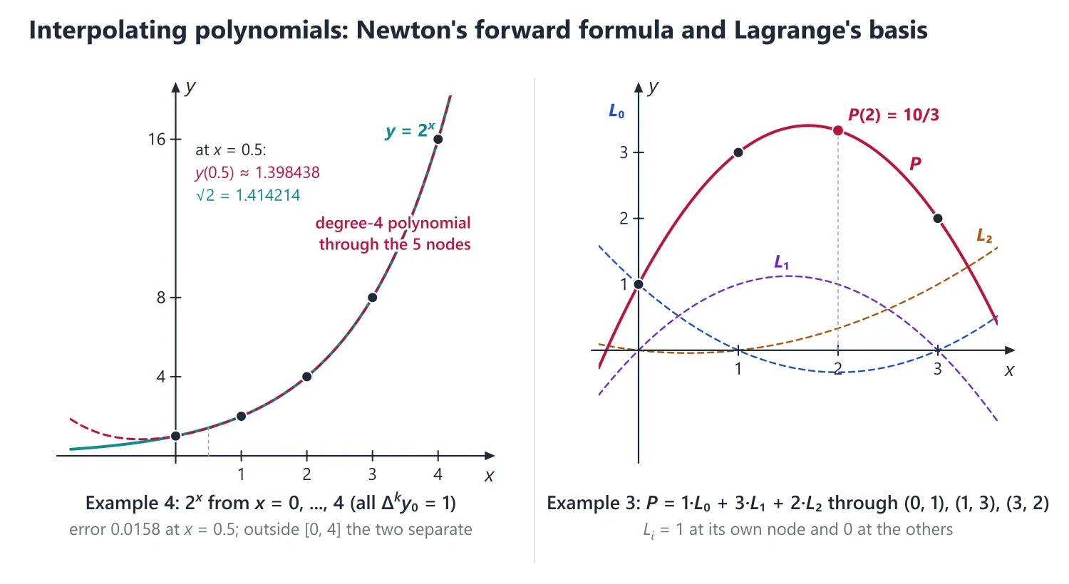
Example 3: through (0, 1), (1, 3), (3, 2), estimate f(2).
L0(2) = (2 − 1)(2 − 3)/((0 − 1)(0 − 3)) = −1/3, L1(2) = (2 − 0)(2 − 3)/((1 − 0)(1 − 3)) = 1, L2(2) = (2 − 0)(2 − 1)/((3 − 0)(3 − 1)) = 1/3.
f(2) ≈ 1 · (−1/3) + 3 · 1 + 2 · (1/3) = 10/3.
Divided differences: f[x0, x1] = (f1 − f0)/(x1 − x0), and P(x) = f0 + (x − x0)f[x0, x1] + (x − x0)(x − x1)f[x0, x1, x2] + ...; a new point can be added without recomputing.
Idea: a divided difference behaves like a scaled derivative: f[x0, ..., xk] = f(k)(ξ)/k! for some ξ among the nodes, and it does not depend on the order of the nodes. For equal spacing f[x0, ..., xk] = Δky0/(k!hk), which turns the divided-difference formula into Newton's forward formula.
Inverse interpolation: interchange the roles of x and y in Lagrange's formula to find the x corresponding to a given y.
Idea: this treats x as a function of y, which makes sense only if y is monotonic over the nodes used; otherwise several x give the same y and the formula picks none of them reliably.
9. Derivation: Backward Formula and the Error Term
Backward formula: with x = xn + ph, y(x) = Epyn, and E−1 = 1 − ∇ gives Ep = (1 − ∇)−p = 1 + p∇ + p(p + 1)∇2/2! + p(p + 1)(p + 2)∇3/3! + ... by the binomial series; applied to yn this is the formula of Section 7 (the forward formula comes the same way from (1 + Δ)p, Section 13).
Error term: fix x (not a node), let w(t) = (t − x0)(t − x1)...(t − xn) and g(t) = f(t) − P(t) − [f(x) − P(x)]w(t)/w(x).
g vanishes at the n + 2 points x0, ..., xn and x, so by Rolle's theorem g′ has n + 1 zeros, g″ has n, ..., and g(n+1) has a zero ξ in the smallest interval containing x and the nodes.
Since P has degree ≤ n, P(n+1) = 0, and w(n+1) = (n + 1)!; so 0 = f(n+1)(ξ) − [f(x) − P(x)](n + 1)!/w(x), which is f(x) − P(x) = f(n+1)(ξ)w(x)/(n + 1)!.
With x = x0 + ph, w(x) = hn+1p(p − 1)...(p − n), which gives the error of Newton's forward formula quoted in Section 13.
10. Choosing the Method
If the data are equally spaced and x is near the start → Newton forward; near the end or just beyond it → Newton backward; in the middle → Stirling (|p| ≤ 1/4) or Bessel/Everett (p near 1/2).
If the points are unequally spaced → Lagrange for a single value, divided differences when the polynomial is wanted in expanded form or more points may be added.
If x is wanted for a given y → inverse interpolation (check that y is monotonic); if derivative values are also given → Hermite interpolation.
If a table entry is missing → with k known values assume degree k − 1, so Δk−1y is constant and Δky = 0 over the range, and expand with E = 1 + Δ.
11. Common Mistakes
Newton's formulae on unequal spacing: they need a constant h; use Lagrange or divided differences instead.
Always starting at the first row: for x deep inside the table, choose x0 as the tabulated point just below x and read that row's diagonal.
Sign errors in Li: compute each Li(x) separately and check that they add up to 1.
Wrong denominator in divided differences: f[x0, x1, x2] = (f[x1, x2] − f[x0, x1])/(x2 − x0), the outermost nodes, not x2 − x1.
Missing-value problems: not stating the assumed degree, or using Δn = 0 with the wrong n; the answer changes with the degree (Example 5).
Link: the trapezoidal and Simpson rules of the next topic are integrals of these interpolating polynomials, and their error terms come from the error formula derived above.
Link: E = ehD is Taylor's theorem (Calculus), the Rolle argument is the one used for Taylor's remainder, and the Li form a basis of the vector space of polynomials of degree ≤ n (Linear Algebra).
12. Worked Examples
Example 4: The table x = 0, 1, 2, 3, 4; y = 1, 2, 4, 8, 16 comes from y = 2x. Estimate y(0.5) by Newton's forward formula and compare with √2.
Since Δ2x = 2x for h = 1, every leading difference is 1: Δy0 = Δ2y0 = Δ3y0 = Δ4y0 = 1.
p = 0.5: y = 1 + 0.5 + (0.5)(−0.5)/2 + (0.5)(−0.5)(−1.5)/6 + (0.5)(−0.5)(−1.5)(−2.5)/24 = 1 + 0.5 − 0.125 + 0.0625 − 0.039063 = 1.398438.
√2 = 1.414214, so the error is 0.0158: 2x is not a polynomial and its differences do not die out, so the terms decrease slowly.
Example 5: Find the missing value in the table x = 0, 1, 2, 3, 4; y = 1, 3, 9, ?, 81, assuming y is a polynomial of degree 3.
For a cubic Δ4y0 = 0, i.e. (E − 1)4 y0 = y4 − 4y3 + 6y2 − 4y1 + y0 = 0.
81 − 4y3 + 54 − 12 + 1 = 0 gives 4y3 = 124, so y3 = 31.
(The data are close to 3x, for which y3 = 27; the answer depends on the assumed degree, which must be stated.)
Example 6: Using Newton's divided difference formula, find the polynomial through (0, 2), (1, 3), (2, 12), (5, 147) and the value f(3).
First divided differences: f[0, 1] = 1, f[1, 2] = 9, f[2, 5] = (147 − 12)/3 = 45.
Second: f[0, 1, 2] = (9 − 1)/2 = 4, f[1, 2, 5] = (45 − 9)/4 = 9. Third: f[0, 1, 2, 5] = (9 − 4)/5 = 1.
P(x) = 2 + x + 4x(x − 1) + x(x − 1)(x − 2) = x3 + x2 − x + 2, so f(3) = 27 + 9 − 3 + 2 = 35.
Example 7: Find a bound for the error of linear interpolation of f(x) = ex between x0 = 0 and x1 = 0.1.
E(x) = f″(ξ)(x − x0)(x − x1)/2, and |(x − x0)(x − x1)| ≤ h2/4 on [x0, x1] (maximum at the midpoint), with h = 0.1.
So |E| ≤ (h2/8) max|f″| = (0.01/8)e0.1 = 0.00125 × 1.105171 ≈ 0.00138.
Check at x = 0.05: the linear value (1 + 1.105171)/2 = 1.052585 and e0.05 = 1.051271 differ by 0.001314, within the bound.
13. Derivations, Central Differences and Hermite Interpolation
Derivation of the forward formula: with x = x0 + ph, y(x) = Epy0 = (1 + Δ)py0; the binomial expansion stopped at Δn is the polynomial of degree n through x0, ..., xn, with error p(p − 1)...(p − n)hn+1f(n+1)(ξ)/(n + 1)!.
Central differences: δ = E1/2 − E−1/2 and μ = (E1/2 + E−1/2)/2; δ2y0 = Δ2y−1. Central formulas use differences on the line through x0 and converge fastest in the middle of a table: Stirling for |p| ≤ 1/4, Bessel and Everett for p near 1/2.
Stirling: yp = y0 + p(Δy0 + Δy−1)/2 + (p2/2!)Δ2y−1 + [p(p2 − 1)/3!](Δ3y−1 + Δ3y−2)/2 + [p2(p2 − 1)/4!]Δ4y−2 + ...
Everett: with q = 1 − p, yp = qy0 + [q(q2 − 1)/3!]δ2y0 + ... + py1 + [p(p2 − 1)/3!]δ2y1 + ..., using only even differences (δ2y0 = Δ2y−1, δ2y1 = Δ2y0).
Hermite (osculating) interpolation: if f and f′ are given at n + 1 distinct nodes, there is a unique polynomial of degree ≤ 2n + 1 matching both, with error f(2n+2)(ξ)∏(x − xi)2/(2n + 2)!; it is the limit of Lagrange interpolation as pairs of nodes coalesce.
Bound when f is not given: state the truncation error as |E(x)| ≤ Mn+1 max|∏(x − xi)|/(n + 1)!, where Mn+1 = max|f(n+1)| on the interval, and find max|∏(x − xi)| by calculus.
14. Past UPSC Questions Solved
Example 8 (UPSC 2021, 15 marks): Derive Newton’s backward difference interpolation formula and also do error analysis.
Let xi = x0 + ih (i = 0, ..., n) and x = xn + ph. Since E−1 = 1 − ∇, y(x) = Epyn = (1 − ∇)−pyn = [1 + p∇ + p(p + 1)/2! ∇2 + ...]yn.
Stopping at ∇n: P(x) = yn + p∇yn + p(p + 1)/2! ∇2yn + ... + p(p + 1)...(p + n − 1)/n! ∇nyn, a polynomial of degree n in x.
Check at x = xn−k (p = −k, 0 ≤ k ≤ n): the j-th coefficient becomes (−1)jC(k, j), zero for j > k, so P = (1 − ∇)kyn = E−kyn = yn−k; P interpolates all n + 1 points.
Error: let w(t) = (t − x0)...(t − xn) and g(t) = f(t) − P(t) − [f(x) − P(x)]w(t)/w(x) for fixed x not a node; g vanishes at the n + 2 points x0, ..., xn, x, so by Rolle's theorem applied repeatedly g(n+1)(ξ) = 0 for some ξ in the interval containing them.
Since P(n+1) = 0 and w(n+1) = (n + 1)!, f(x) − P(x) = w(x)f(n+1)(ξ)/(n + 1)!; with x − xn−k = (p + k)h this is E(x) = p(p + 1)...(p + n)hn+1f(n+1)(ξ)/(n + 1)! ≈ [p(p + 1)...(p + n)/(n + 1)!]∇n+1yn.
Answer: Newton's backward formula as above, with error p(p + 1)...(p + n)hn+1f(n+1)(ξ)/(n + 1)!, which is small for small |p|, i.e. near the end of the table.
Example 9 (UPSC 2017, 15 marks): For given equidistant values u−1, u0, u1 and u2, a value is interpolated by Lagrange's formula. Show that it may be written in the form
ux = yu0 + xu1 + (y(y2 − 1)/3!) Δ2u−1 + (x(x2 − 1)/3!) Δ2u0,
where x + y = 1.
Take h = 1, nodes −1, 0, 1, 2 and y = 1 − x; the right side R(x) is then a polynomial of degree ≤ 3 in x. By uniqueness, R is Lagrange's cubic through the four points if R(k) = uk for k = −1, 0, 1, 2.
x = 0 (y = 1): both cubic terms vanish since y(y2 − 1) = 0 = x(x2 − 1), so R = u0; x = 1 (y = 0): R = u1.
x = −1 (y = 2): R = 2u0 − u1 + (2 · 3/6)Δ2u−1 = 2u0 − u1 + (u1 − 2u0 + u−1) = u−1.
x = 2 (y = −1): R = −u0 + 2u1 + (2 · 3/6)Δ2u0 = −u0 + 2u1 + (u2 − 2u1 + u0) = u2.
Answer: R agrees with u at all four nodes, so it is the Lagrange interpolating cubic; this is Everett's formula up to second differences.
Example 10 (UPSC 2020, 15 marks): Write the three point Lagrangian interpolating polynomial relative to the points x0, x0 + ε and x1. Then by taking the limit ε → 0, establish the relation f(x) = ((x1 − x)(x + x1 − 2x0)/(x1 − x0)2) f(x0) + ((x − x0)(x1 − x)/(x1 − x0)) f′(x0) + ((x − x0)2/(x1 − x0)2) f(x1) + E(x) where E(x) = (1/6)(x − x0)2(x − x1)f‴(ξ) is the error function and min.(x0, x0 + ε, x1) < ξ < max.(x0, x0 + ε, x1)
Lagrange: Pε(x) = f(x0)(x − x0 − ε)(x − x1)/(−ε(x0 − x1)) + f(x0 + ε)(x − x0)(x − x1)/(ε(x0 + ε − x1)) + f(x1)(x − x0)(x − x0 − ε)/((x1 − x0)(x1 − x0 − ε)).
By uniqueness it equals the Newton form f(x0) + (x − x0)f[x0, x0 + ε] + (x − x0)(x − x0 − ε)f[x0, x0 + ε, x1]; as ε → 0, f[x0, x0 + ε] → f′(x0) and f[x0, x0 + ε, x1] → (f1 − f0 − hf′0)/h2, where h = x1 − x0.
So the limit is P(x) = f0 + (x − x0)f′0 + (x − x0)2(f1 − f0 − hf′0)/h2.
Collecting: coefficient of f0 is 1 − (x − x0)2/h2 = (x1 − x)(x + x1 − 2x0)/h2; of f′0 is (x − x0) − (x − x0)2/h = (x − x0)(x1 − x)/h; of f1 is (x − x0)2/h2.
Error: f(x) − Pε(x) = (x − x0)(x − x0 − ε)(x − x1)f‴(ξε)/3!, and letting ε → 0 (f‴ continuous) gives E(x) = (1/6)(x − x0)2(x − x1)f‴(ξ).
Answer: the stated relation, a Hermite-type quadratic matching f(x0), f′(x0) and f(x1).
Example 11 (UPSC 2016, 20 marks): Let f(x) = e2x cos 3x, for x ∈ [0, 1]. Estimate the value of f(0·5) using Lagrange interpolating polynomial of degree 3 over the nodes x = 0, x = 0·3, x = 0·6 and x = 1. Also, compute the error bound over the interval [0, 1] and the actual error E(0·5).
Values: f(0) = 1, f(0.3) = 1.132647, f(0.6) = −0.754338, f(1) = −7.315110.
At x = 0.5: L0 = (0.2)(−0.1)(−0.5)/((−0.3)(−0.6)(−1)) = −0.055556, L1 = (0.5)(−0.1)(−0.5)/((0.3)(−0.3)(−0.7)) = 0.396825, L2 = (0.5)(0.2)(−0.5)/((0.6)(0.3)(−0.4)) = 0.694444, L3 = (0.5)(0.2)(−0.1)/((1)(0.7)(0.4)) = −0.035714.
P3(0.5) = −0.055556 + 0.396825(1.132647) + 0.694444(−0.754338) − 0.035714(−7.315110) = 0.131316.
Error term E(x) = f⁗(ξ)x(x − 0.3)(x − 0.6)(x − 1)/4!; since f = Re e(2+3i)x, f⁗ = Re[(2 + 3i)4e(2+3i)x] = e2x(120 sin 3x − 119 cos 3x).
On [0, 1], max|f⁗| ≈ 998.3 (near x = 0.98; the cruder bound |2 + 3i|4e2 = 169e2 ≈ 1249 also serves) and max|x(x − 0.3)(x − 0.6)(x − 1)| ≈ 0.01755 (near x = 0.855).
Error bound on [0, 1]: |E| ≤ 998.3 × 0.01755/24 ≈ 0.730; at x = 0.5, |w(0.5)| = 0.005 gives |E(0.5)| ≤ 998.3 × 0.005/24 ≈ 0.416.
Answer: f(0.5) ≈ 0.131316; actual f(0.5) = e cos 1.5 = 0.192284, so E(0.5) = 0.060968, well within the bound 0.730.
Example 12 (UPSC 2025, 15 marks): Find the unique polynomial of degree 2 or less which fits the following data:
x : 0, 1, 3
f(x) : 1, 3, 55
Also obtain the bound on the truncation error.
Lagrange: P(x) = 1 · (x − 1)(x − 3)/3 + 3 · x(x − 3)/(−2) + 55 · x(x − 1)/6.
Coefficient of x2: 1/3 − 3/2 + 55/6 = 8; of x: −4/3 + 9/2 − 55/6 = −6; constant 1. So P(x) = 8x2 − 6x + 1 (check: P(0) = 1, P(1) = 3, P(3) = 55).
Uniqueness: two such polynomials would differ by a polynomial of degree ≤ 2 with the three roots 0, 1, 3, hence by zero.
Truncation error E(x) = f‴(ξ)x(x − 1)(x − 3)/3!. For w(x) = x3 − 4x2 + 3x, w′ = 3x2 − 8x + 3 = 0 at x = (4 ± √7)/3 = 0.4514, 2.2153, where |w| = 0.6311 and 2.1126.
Answer: P(x) = 8x2 − 6x + 1; for 0 ≤ x ≤ 3, |E(x)| ≤ 2.1126 M3/6 ≈ 0.352 M3, where M3 = max|f‴| on [0, 3].
15. Practice Exercises
Exercise 1 (basic): Form the difference table for y = 2, 5, 10, 17 at x = 0, 1, 2, 3 and state the degree of the data.
Answer: Δy = 3, 5, 7; Δ2y = 2, 2; Δ3y = 0: degree 2 (y = x2 + 2x + 2).
Exercise 2 (basic): With h = 1, find Δ(x2) and Δ2(x2).
Answer: Δx2 = (x + 1)2 − x2 = 2x + 1 and Δ2x2 = 2 = 2! × 1 × 12.
Exercise 3 (basic): Given f(1) = 3 and f(3) = 7, estimate f(2) by linear Lagrange interpolation.
Answer: L0(2) = L1(2) = 1/2, so f(2) ≈ 5.
Exercise 4 (standard): From x = 0, 1, 2, 3 and y = 1, 2, 11, 34, find the interpolating polynomial by Newton's forward formula and y(1.5).
Answer: Δy0 = 1, Δ2y0 = 8, Δ3y0 = 6; P(x) = x3 + x2 − x + 1 and y(1.5) = 5.125.
Exercise 5 (standard): From the same table, find y(2.5) by Newton's backward formula.
Answer: ∇y3 = 23, ∇2y3 = 14, ∇3y3 = 6, p = −0.5: y = 34 − 11.5 − 1.75 − 0.375 = 20.375.
Exercise 6 (standard): Find the quadratic through (0, −1), (1, 1), (3, 23) by Lagrange's formula, and f(2).
Answer: P(x) = 3x2 − x − 1, so f(2) ≈ 9.
Exercise 7 (standard): Using Newton's divided differences for (1, 1), (2, 5), (4, 17), (5, 26), estimate f(3).
Answer: f[1, 2] = 4, f[1, 2, 4] = 2/3, f[1, 2, 4, 5] = 1/12; P(3) = 1 + 8 + 4/3 − 1/6 = 61/6 ≈ 10.1667.
Exercise 8 (UPSC level): The table x = 0, 1, 2, 3, 4, 5; y = 1, 3, ?, 31, ?, 131 comes from a cubic. Find the two missing values.
Answer: Δ4y0 = 0 gives y4 + 6y2 = 135 and Δ4y1 = 0 gives y4 + y2 = 80, so y2 = 11 and y4 = 69 (the cubic is x3 + x + 1).
Exercise 9 (UPSC level): A table of sin x (x in radians) is to be used with linear interpolation. What step h guarantees an interpolation error at most 5 × 10⁻⁷?
Answer: |E| ≤ h2M2/8 with M2 = 1, so h2/8 ≤ 5 × 10⁻⁷ gives h ≤ 0.002.
Exercise 10 (UPSC level): From x = 1, 2, 3 and y = −2, 1, 6, estimate by inverse Lagrange interpolation the x at which y = 0.
Answer: y is increasing, so x = ∑xiLi(0) with Li built on y: 1(0.25) + 2(0.8) + 3(−0.05) = 1.7 (the data come from x2 − 3, whose root is 1.7321).
| x | y | Δy | Δ2y | Δ3y |
|---|---|---|---|---|
| 0 | 0 | 1 | 6 | 6 |
| 1 | 1 | 7 | 12 | — |
| 2 | 8 | 19 | — | — |
| 3 | 27 | — | — | — |
| Form of the problem | Method | Watch out for |
|---|---|---|
| Equal spacing, x near the start | Newton forward, p = (x − x0)/h | Use the downward diagonal |
| Equal spacing, x near the end | Newton backward, p = (x − xn)/h | p is negative inside the table |
| Equal spacing, x in the middle | Stirling or Bessel/Everett | Central differences on the line of x0 |
| Unequal spacing, one value | Lagrange | Check ∑Li = 1 |
| Unequal spacing, polynomial wanted | Newton divided differences | Divide by the outermost nodes |
| x for a given y | Inverse interpolation | y must be monotonic |
| f and f′ given | Hermite | Degree up to 2n + 1 |
Mains points
- Expect a numerical question: build the difference table, choose forward or backward formula according to the position of x, and state p clearly.
- Lagrange's formula is often asked with unequally spaced data, sometimes to find the polynomial itself; simplify it fully.
- Derivations of Newton's forward formula (via E = 1 + Δ) and the error term of Lagrange interpolation are standard theory parts.
- Mention why the chosen formula suits the data (equal or unequal spacing, beginning or end of the table).
- Common mistake: using p = (x − x0)/h with the backward formula, or reading the wrong diagonal of the difference table.
Did you know?
- Interpolating many equally spaced points with one high-degree polynomial can oscillate wildly near the ends (Runge's phenomenon, for 1/(1 + 25x2) on [−1, 1]); this is why piecewise or Chebyshev-node interpolation is used in practice.
Numerical Integration and Numerical Solution of ODEs
Newton–Cotes rules integrate the interpolating polynomial over equal strips: the trapezoidal rule (error O(h2)) and Simpson's 1/3 and 3/8 rules (error O(h4)). Gaussian quadrature chooses nodes and weights so that n points integrate polynomials of degree 2n − 1 exactly. For y′ = f(x, y), Euler's method is first order and the classical fourth-order Runge-Kutta method matches the Taylor series up to h4 without derivatives of f.
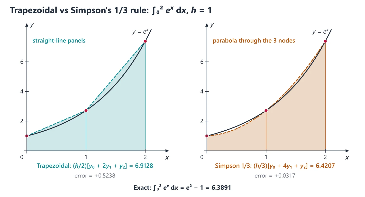
1. Understanding the Trapezoidal and Simpson's Rules
Why we need it: many integrals, such as ∫e−x2 dx, have no elementary antiderivative, and in experiments the integrand is known only as a table of values. We need to approximate ∫ab f(x) dx from the values yi = f(xi).
In words: divide [a, b] into n strips of width h = (b − a)/n. The trapezoidal rule replaces the curve on each strip by its chord; Simpson's 1/3 rule replaces it on each pair of strips by the parabola through three points.
Adding the pieces gives the weights: trapezoidal (h/2)(1, 2, 2, ..., 2, 1), Simpson (h/3)(1, 4, 2, 4, ..., 4, 1), the latter only for even n. The errors are O(h2) and O(h4), so halving h cuts them by about 4 and 16.
First example, slowly: evaluate ∫12 dx/x with h = 0.25 by both rules and compare with ln 2 = 0.693147.
Step 1: n = (2 − 1)/0.25 = 4 strips (even, so Simpson's 1/3 rule is allowed); the nodes are 1, 1.25, 1.5, 1.75, 2.
Step 2: the ordinates are 1, 0.8, 0.666667, 0.571429, 0.5.
Step 3: trapezoidal: (0.25/2)[1 + 0.5 + 2(0.8 + 0.666667 + 0.571429)] = 0.125 × 5.576190 = 0.697024.
Step 4: Simpson: (0.25/3)[1 + 0.5 + 4(0.8 + 0.571429) + 2(0.666667)] = (0.25/3) × 8.319048 = 0.693254.
Step 5: errors: trapezoidal 0.693147 − 0.697024 = −0.003877, Simpson −0.000107, about 36 times smaller for the same five values.
Step 6: notice the sign: 1/x is convex (f″ > 0), every chord lies above the curve, and the trapezoidal rule overestimates, as its error term −(b − a)h2f″(ξ)/12 predicts.
Non-example: with n = 3 strips Simpson's 1/3 rule cannot be applied: the strips cannot be grouped in pairs, and the weight pattern 1, 4, 2, ..., 4, 1 does not fit four ordinates. The condition that fails is 'n even'; use the 3/8 rule on three strips instead.
Building up: both rules are integrals of Newton's forward polynomial over one or two strips; Simpson's rule is exact even for cubics because the cubic term integrates to zero over the pair of strips ('Derivation: Trapezoidal and Simpson's Rules with Error Terms' below).
Where it is used: tabulated data such as the speed of a train (UPSC 2018, 2022), estimates of ln 2 or π, and 'how many sub-intervals for a given accuracy' questions.
2. Understanding Degree of Precision and Gaussian Quadrature
Why we need it: to compare quadrature rules, and to design new ones, we need a single measure of how good a rule is. If each function evaluation is expensive, we also want the best possible accuracy from very few points.
In words: a rule has degree of precision m if it integrates 1, x, ..., xm exactly but not xm+1. Since any smooth f is close to its Taylor polynomial, a higher m usually means a smaller error.
Newton–Cotes rules fix equally spaced nodes and choose only the weights. Gauss–Legendre rules choose both nodes and weights; with n nodes that is 2n free numbers, enough for degree 2n − 1.
First example, slowly: find the degree of precision of the midpoint rule ∫−11 f dt ≈ 2f(0), then evaluate ∫01 ex dx by the two-point Gauss rule.
Step 1: f = 1: exact value 2, rule 2. f = t: exact 0, rule 0. f = t2: exact 2/3, rule 0. So the midpoint rule has degree 1, the same as the trapezoidal rule, with only one point.
Step 2: for Gauss, map [0, 1] to [−1, 1] by x = (t + 1)/2, dx = dt/2, so ∫01 ex dx = (1/2)∫−11 e(t+1)/2 dt.
Step 3: the nodes t = ±1/√3 = ±0.577350 map to x = 0.211325 and 0.788675, with weights 1.
Step 4: e0.211325 = 1.235314 and e0.788675 = 2.200479.
Step 5: I ≈ (1/2)(1.235314 + 2.200479) = 1.717896, while e − 1 = 1.718282.
Step 6: the error 0.000386 from two function values is smaller than that of the trapezoidal rule with four strips (five values, error about −0.0090).
Non-example: two equally spaced points ±1 with weights 1, 1 give the trapezoidal rule 2 × [f(−1) + f(1)]/2, which already fails for t2 (it gives 2 instead of 2/3): degree 1, not 3. The condition that fails is 'nodes at the zeros of the Legendre polynomial'; only those nodes reach degree 2n − 1.
Building up: the method of undetermined coefficients (demand exactness for 1, t, t2, t3) gives the two-point nodes ±1/√3 ('Two-point Gauss rule derived' below); testing the next power gives the error constant and the error term C f(m+1)(ξ)/(m + 1)!.
Where it is used: 'derive the two-point Gauss rule and use it' (UPSC 2016), 'find the constants so that the formula is exact for polynomials of highest degree' (UPSC 2018, 2020, 2025), and weighted rules such as ∫f(x)dx/√(x(1 − x)).
3. Understanding Euler's Method and Local versus Global Error
Why we need it: most initial value problems y′ = f(x, y), y(x0) = y0 cannot be solved in closed form. We need to march the solution forward step by step, and to understand how the errors of the steps accumulate.
In words: at (xn, yn) the equation gives the slope f(xn, yn) of the solution through that point. Euler's method follows this tangent for one step: yn+1 = yn + hf(xn, yn).
The local error is the error made in one step starting from exact values, about h2y″/2. The global error at a fixed point x is the accumulated error after (x − x0)/h steps, about (1/h) × h2 = h: so Euler's method is of first order.
First example, slowly: apply Euler's method to y′ = y, y(0) = 1 up to x = 0.3, first with h = 0.1 and then with h = 0.05.
Step 1: here f(x, y) = y, so each step is yn+1 = yn + hyn = (1 + h)yn.
Step 2: with h = 0.1: y1 = 1.1, y2 = 1.21, y3 = 1.331.
Step 3: the exact value is e0.3 = 1.349859, so the global error is 0.018859.
Step 4: with h = 0.05 we need six steps: y6 = 1.056 = 1.340096, with error 0.009763.
Step 5: halving h roughly halved the error (0.0189 to 0.0098): this is what 'first order' means.
Step 6: notice the bias: y is convex, every tangent lies below the curve, so Euler's values are always too small here.
Non-example: for y′ = −50y, y(0) = 1 the solution e−50x decays at once, but Euler with h = 0.1 gives yn+1 = (1 − 5)yn, i.e. −4, 16, −64, ...: the numbers explode. The step is too large for this stiff equation; the condition that fails is |1 + hλ| < 1 (here h < 0.04).
Building up: Taylor's theorem gives the local error (h2/2)y″(ξ), and a Lipschitz condition on f keeps the propagated errors bounded by a factor eL(b − a), which gives global error O(h) ('Euler's global error' below).
Averaging the slopes at both ends of the step (Heun's modified Euler method) cancels the h2 term and gives a second-order method; the next lesson goes further.
Where it is used: 'apply Euler's method and compare with the exact solution' questions, the predictor step of predictor-corrector methods, and the meaning of the order of any ODE method.
4. Understanding the Runge-Kutta Methods
Why we need it: Euler's method needs very small steps for good accuracy, and the Taylor series method needs derivatives of f, which can be messy. Runge-Kutta methods reach high order using only values of f.
In words: inside each step the method samples the slope at several trial points and takes a weighted average. In RK4, k1 is the slope at the start, k2 and k3 are two estimates at the midpoint, and k4 is at the end; the update uses weights 1, 2, 2, 1 divided by 6.
The weights are chosen so that yn+1 agrees with the Taylor series of the true solution up to the h4 term: local error O(h5), global error O(h4).
First example, slowly: take one RK4 step with h = 0.1 for y′ = y, y(0) = 1, and compare with e0.1.
Step 1: k1 = hf(0, 1) = 0.1 × 1 = 0.1.
Step 2: k2 = hf(0.05, 1 + k1/2) = 0.1 × 1.05 = 0.105.
Step 3: k3 = hf(0.05, 1 + k2/2) = 0.1 × 1.0525 = 0.10525.
Step 4: k4 = hf(0.1, 1 + k3) = 0.1 × 1.10525 = 0.110525.
Step 5: y1 = 1 + (0.1 + 0.21 + 0.2105 + 0.110525)/6 = 1 + 0.631025/6 = 1.105171.
Step 6: e0.1 = 1.105171 to six decimals. In fact y1 = 1 + h + h2/2 + h3/6 + h4/24 exactly: the Taylor series up to h4, as promised.
Non-example: the rule yn+1 = yn + k2 with k2 = hf(xn + h, yn + k1) looks like a two-stage Runge-Kutta method, but it is only of first order: for y′ = y it gives 1 + h + h2 instead of 1 + h + h2/2. In the family w1k1 + w2k2 with k2 at xn + αh, second order needs w1 + w2 = 1 and αw2 = 1/2; here αw2 = 1.
Building up: matching the Taylor series term by term gives the order conditions ('Second-order Runge-Kutta family' below); when f depends on x only, RK4 collapses to Simpson's rule on the step.
For a system or a second-order equation, every stage computes the k's of all components from the same old values before any component is updated.
Where it is used: 'use the fourth-order Runge-Kutta method to find y(0.2)' questions, the RK4 algorithm of the last topic, and as the default accurate method whenever a question asks only for accuracy.
5. Newton–Cotes Rules (h = (b − a)/n, yi = f(xi))
Trapezoidal rule: ∫ab f(x) dx ≈ (h/2)[y0 + 2(y1 + ... + yn−1) + yn]; error −(b − a)h2f″(ξ)/12; exact for linear f.
Idea: on each strip the curve is replaced by its chord, so the rule adds the areas of trapezia (see the figure above). For a convex function (f″ > 0) every chord lies above the curve and the rule overestimates, which is what the negative error I − T = −(b − a)h2f″(ξ)/12 says.
Simpson's 1/3 rule (n even): (h/3)[y0 + 4(y1 + y3 + ...) + 2(y2 + y4 + ...) + yn]; error −(b − a)h4f(4)(ξ)/180; exact for cubics.
Idea: each pair of strips is replaced by the parabola through three points, which hugs a smooth curve far better than chords (see the figure above). It is exact even for cubics, one degree more than the parabola it fits, because the cubic part of the error cancels by symmetry over the double strip (derived below).
Simpson's 3/8 rule (n a multiple of 3): (3h/8)[y0 + 3y1 + 3y2 + 2y3 + 3y4 + 3y5 + 2y6 + ... + yn]; error −(b − a)h4f(4)(ξ)/80.
Idea: for the same h the 3/8 rule's error constant 1/80 is larger than Simpson's 1/180, so the 1/3 rule is preferred when n is even; the 3/8 rule is useful when n is odd: apply it to three strips and the 1/3 rule to the remaining even number.
All three follow by integrating Newton's forward formula over 1, 2 or 3 strips and adding.
Example 1: ∫01 dx/(1 + x2) = π/4 ≈ 0.785398 with h = 0.25: y = 1, 0.941176, 0.8, 0.64, 0.5.
Trapezoidal: 0.125[1.5 + 2(2.381176)] = 0.782794. Simpson 1/3: (0.25/3)[1.5 + 4(1.581176) + 2(0.8)] = 0.785392, giving π ≈ 3.14157.
6. Gaussian Quadrature
∫−11 f(t) dt ≈ ∑i=1n wif(ti), where the nodes ti are the zeros of the Legendre polynomial Pn; the rule is exact for all polynomials of degree ≤ 2n − 1.
Idea: Newton–Cotes rules fix the nodes and choose only the weights; Gauss chooses both, so n nodes and n weights give 2n free parameters, enough to integrate 1, t, ..., t2n−1 exactly. It never uses the end points, which helps when f is awkward there.
Two-point rule: t = ±1/√3, w = 1, so ∫−11 f(t) dt ≈ f(−1/√3) + f(1/√3).
Three-point rule: t = 0, ±√(3/5) with weights 8/9, 5/9, 5/9.
Any interval: x = [(b − a)t + (b + a)]/2 gives ∫ab f(x) dx = ((b − a)/2)∫−11 f(x(t)) dt.
Example 2: ∫01 x3 dx by the two-point rule: x = (t + 1)/2 gives (1/2)[(0.211325)3 + (0.788675)3] = (1/2)(0.009437 + 0.490563) = 0.25, exact as expected for degree 3.
7. Euler's Method for y′ = f(x, y), y(x0) = y0
yn+1 = yn + hf(xn, yn), xn+1 = xn + h; local error O(h2), global error O(h), so it is first order.
Idea: each step follows the tangent to the solution curve through (xn, yn); the true curve bends away by about h2y″/2 in one step, and over (b − a)/h steps these local errors add up to O(h). Halving h roughly halves the error (Example 8).
Modified Euler (Heun) method: y* = yn + hf(xn, yn), then yn+1 = yn + (h/2)[f(xn, yn) + f(xn+1, y*)]; this is a second-order Runge-Kutta method.
Idea: Heun averages the slopes at both ends of the step, which is the trapezoidal rule applied to y′ = f; the Euler predictor supplies the unknown end value y*.
8. Runge-Kutta Methods
Fourth-order RK: k1 = hf(xn, yn), k2 = hf(xn + h/2, yn + k1/2), k3 = hf(xn + h/2, yn + k2/2), k4 = hf(xn + h, yn + k3).
yn+1 = yn + (k1 + 2k2 + 2k3 + k4)/6; local error O(h5), global error O(h4).
Idea: k1, ..., k4 are slope samples at the start, twice at the midpoint and at the end of the step; when f depends on x only they become hf(xn), hf(xn + h/2) (twice) and hf(xn + h), and the update is (h/6)[f(xn) + 4f(xn + h/2) + f(xn + h)], which is Simpson's rule. That explains the weights 1, 2, 2, 1.
Example 3: y′ = x + y, y(0) = 1, h = 0.1; the exact solution is y = 2ex − x − 1, so y(0.1) = 1.110342.
Euler: y1 = 1 + 0.1(0 + 1) = 1.1. Heun: y* = 1.1, y1 = 1 + 0.05(1 + 1.2) = 1.11.
RK4: k1 = 0.1, k2 = 0.1(0.05 + 1.05) = 0.11, k3 = 0.1(0.05 + 1.055) = 0.1105, k4 = 0.1(0.1 + 1.1105) = 0.12105.
y1 = 1 + (0.1 + 0.22 + 0.221 + 0.12105)/6 = 1.110342, correct to six decimals.
Higher-order equations are written as first-order systems and the same formulas are applied to each component.
Idea: y″ = g(x, y, y′) becomes y′ = z, z′ = g(x, y, z); each RK stage computes the k for y and the k for z from the same old values before either is updated.
9. Derivation: Trapezoidal and Simpson's Rules with Error Terms
Trapezoidal, one strip: with x = x0 + ph, ∫x0x1 f dx ≈ h∫01(y0 + pΔy0) dp = h(y0 + Δy0/2) = (h/2)(y0 + y1).
Its error is ∫ f″(ξx)(x − x0)(x − x1)/2 dx; the factor (x − x0)(x − x1) keeps one sign, so by the mean value theorem for integrals it equals (f″(η)/2)∫x0x1(x − x0)(x − x1) dx = (f″(η)/2)(−h3/6) = −h3f″(η)/12.
Composite rule: adding n strips gives −(h3/12)∑f″(ηi) = −(nh3/12)f″(ξ) (the average of the f″(ηi) is a value f″(ξ) by the intermediate value theorem), and nh = b − a gives −(b − a)h2f″(ξ)/12.
Simpson, two strips: h∫02[y0 + pΔy0 + p(p − 1)Δ2y0/2] dp = h[2y0 + 2Δy0 + Δ2y0/3]; with Δy0 = y1 − y0 and Δ2y0 = y2 − 2y1 + y0 this is (h/3)(y0 + 4y1 + y2).
The next term of Newton's formula, p(p − 1)(p − 2)Δ3y0/6, integrates to zero because ∫02p(p − 1)(p − 2) dp = 0 (odd about p = 1), so the rule is exact for cubics.
The error constant for f = x4 on [−h, h] is I − Q = 2h5/5 − (h/3)(2h4) = −4h5/15; dividing by 4! gives the panel error −h5f⁗(η)/90, and n/2 panels with nh = b − a give −(b − a)h4f⁗(ξ)/180.
Euler's global error: Taylor's theorem gives y(xn+1) = y(xn) + hy′(xn) + (h2/2)y″(ξ), so one step errs by O(h2); there are (b − a)/h steps, so the accumulated error is O(h) when f is Lipschitz in y (errors are amplified by at most a fixed factor eL(b − a)).
10. Choosing the Method
If the integrand is a table with n strips → n even: Simpson 1/3; n a multiple of 3: Simpson 3/8 is allowed; n odd and not a multiple of 3: 3/8 on three strips and 1/3 on the rest; otherwise trapezoidal.
If f is a formula and only a few evaluations are allowed → Gauss–Legendre after mapping [a, b] to [−1, 1].
If an accuracy is prescribed → bound the relevant derivative on [a, b] and solve the error formula for h, then round n up (and make it even for Simpson).
If an ODE question names the method → follow it exactly (Euler, modified Euler, RK2, RK4); if it only asks for accuracy → RK4 is the default; if f is easy to differentiate → the Taylor series method is also acceptable.
If the ODE is of second order → rewrite as a first-order system and advance y and y′ together.
11. Common Mistakes
Simpson's 1/3 rule with an odd number of strips: the rule needs pairs of strips; check n before starting.
Wrong weight pattern: the end ordinates get weight 1, and the interior ones alternate 4, 2, 4, ..., 4, starting and ending with 4.
Forgetting the factor (b − a)/2 when mapping [a, b] to [−1, 1] in Gauss quadrature.
RK4 slips: using yn + k1 instead of yn + k1/2 in k2, or dropping the factor h from the k's.
Systems: updating y before computing the slope for y′ in the same step, which mixes old and new values.
Error bounds at one point: the bound needs max|f″| (or max|f⁗|) over the whole interval, found by calculus as in Example 6.
Link: every Newton–Cotes rule is the integral of the interpolating polynomial of the previous topic, and its error is Lagrange's error formula integrated over the strip.
Link: Runge-Kutta methods match the Taylor series of the solution (Calculus), and the existence and uniqueness theorem for y′ = f(x, y) (Ordinary Differential Equations) is what guarantees there is a solution to approximate; for y′ = f(x) RK4 reduces to Simpson's rule.
12. Worked Examples
Example 4: Evaluate ∫06 dx/(1 + x2) with h = 1 by the trapezoidal, Simpson's 1/3 and Simpson's 3/8 rules, and compare with tan−16.
Ordinates at x = 0, 1, ..., 6: 1, 0.5, 0.2, 0.1, 0.058824, 0.038462, 0.027027.
Trapezoidal: (1/2)[1.027027 + 2(0.897286)] = 1.410799. Simpson 1/3: (1/3)[1.027027 + 4(0.638462) + 2(0.258824)] = 1.366173.
Simpson 3/8: (3/8)[1.027027 + 3(0.5 + 0.2 + 0.058824 + 0.038462) + 2(0.1)] = 1.357081.
Exact value tan−16 = 1.405648. Here the trapezoidal rule happens to be closest: with h = 1 the higher derivatives of 1/(1 + x2) near 0 are large, so the Simpson error terms are not small; halving h restores Simpson's advantage.
Example 5: Evaluate ∫12 dx/x by the two-point Gauss-Legendre rule.
x = (t + 3)/2, dx = dt/2, so I = ∫−11 dt/(t + 3).
I ≈ 1/(3 − 1/√3) + 1/(3 + 1/√3) = 6/(9 − 1/3) = 9/13 = 0.692308.
ln 2 = 0.693147, so the error is 0.00084 with only two function values.
Example 6: How many sub-intervals are needed to evaluate ∫01 e−x2 dx by the trapezoidal rule with error at most 0.5 × 10⁻⁴?
|E| ≤ (b − a)h2 max|f″|/12, with f″(x) = (4x2 − 2)e−x2.
f‴(x) = (12x − 8x3)e−x2 > 0 on (0, 1], so f″ increases from −2 to 2/e; hence max|f″| = 2 (at x = 0) and |E| ≤ h2/6.
h2/6 ≤ 0.5 × 10⁻⁴ needs h ≤ 0.017321, so n = 1/h ≥ 57.7: take n = 58.
Example 7: Use the fourth-order Runge-Kutta method with h = 0.2 to find y(0.2) for dy/dx = (y − x)/(y + x), y(0) = 1.
k1 = 0.2 f(0, 1) = 0.2; k2 = 0.2 f(0.1, 1.1) = 0.2(1.0/1.2) = 0.166667.
k3 = 0.2 f(0.1, 1.083333) = 0.2(0.983333/1.183333) = 0.166197; k4 = 0.2 f(0.2, 1.166197) = 0.2(0.966197/1.366197) = 0.141443.
y(0.2) = 1 + (0.2 + 0.333333 + 0.332394 + 0.141443)/6 = 1.167862.
Example 8: Apply Euler's method with h = 0.1 to dy/dx = −2xy, y(0) = 1, up to x = 0.3, and compare with the exact solution y = e−x2.
y1 = 1 + 0.1(−2 · 0 · 1) = 1; y2 = 1 + 0.1(−2 · 0.1 · 1) = 0.98; y3 = 0.98 + 0.1(−2 · 0.2 · 0.98) = 0.9408.
Exact y(0.3) = e−0.09 = 0.913931, so the error is 0.0269; it is roughly halved by halving h, as expected for a first-order method.
13. Degree of Precision, Derivations and More ODE Methods
Degree of precision: a rule Q for I(f) = ∫ w(x)f(x) dx has degree of precision m if it is exact for 1, x, ..., xm but not for xm+1.
Method of undetermined coefficients: write the rule with unknown weights (and nodes), demand exactness for f = 1, x, x2, ... until the unknowns are fixed, then test the next power to find m.
Error term: for the standard rules (whose Peano kernel keeps one sign), E = I − Q = C f(m+1)(ξ)/(m + 1)!, where the error constant is C = I(xm+1) − Q(xm+1); for a single panel of width h the error is O(hm+2).
Two-point Gauss rule derived: require ∫−11 f ≈ w1f(t1) + w2f(t2) exact for 1, t, t2, t3: w1 + w2 = 2, w1t1 + w2t2 = 0, w1t12 + w2t22 = 2/3, w1t13 + w2t23 = 0.
Subtracting t22 times the second equation from the fourth gives w1t1(t12 − t22) = 0, so t2 = −t1 (distinct non-zero nodes); then w1 = w2 = 1 and 2t12 = 2/3, so t = ±1/√3. For f = t4, C = 2/5 − 2/9 = 8/45, so the error is f⁗(ξ)/135.
Modified Euler as predictor-corrector: predictor yn+1(0) = yn + hf(xn, yn); corrector yn+1(k+1) = yn + (h/2)[f(xn, yn) + f(xn+1, yn+1(k))], repeated until two values agree; local error O(h3).
Second-order Runge-Kutta family: yn+1 = yn + w1k1 + w2k2, k1 = hf(xn, yn), k2 = hf(xn + αh, yn + αk1); matching the Taylor series up to h2 requires w1 + w2 = 1 and αw2 = 1/2 (α = 1: Heun; α = 1/2: midpoint method).
Taylor series method: yn+1 = yn + hy′n + (h2/2!)y″n + (h3/3!)y‴n + ..., where y″, y‴ are found by differentiating the equation; Runge-Kutta methods reproduce these terms without derivatives of f.
14. Past UPSC Questions Solved
Example 9 (UPSC 2016, 15 marks): For an integral ∫−11 f(x) dx, show that the two-point Gauss quadrature rule is given by ∫−11 f(x) dx = f(1/√3) + f(−1/√3). Using this rule, estimate ∫24 2x ex dx.
The derivation in the previous sub-section gives ∫−11 f(x) dx ≈ f(−1/√3) + f(1/√3), exact for all cubics.
For ∫24 2xex dx put x = t + 3 (dx = dt, t ∈ [−1, 1]): I = ∫−11 g(t) dt with g(t) = 2(t + 3)et+3.
g(1/√3) = 2(3.577350)e3.577350 = 255.985 and g(−1/√3) = 2(2.422650)e2.422650 = 54.634.
Answer: I ≈ 310.62; the exact value 2[(x − 1)ex]24 = 6e4 − 2e2 = 312.81, an error of about 0.7%.
Example 10 (UPSC 2017, 20 marks): Derive the formula
∫ab y dx = (3h/8)[(y0 + yn) + 3(y1 + y2 + y4 + y5 + ... + yn−1) + 2(y3 + y6 + ... + yn−3)].
Is there any restriction on n? State that condition. What is the error bound in the case of Simpson's 3/8 rule?
With x = x0 + ph and Newton's forward formula up to Δ3: ∫x0x3 y dx = h∫03[y0 + pΔy0 + p(p − 1)/2 Δ2y0 + p(p − 1)(p − 2)/6 Δ3y0] dp = h[3y0 + (9/2)Δy0 + (9/4)Δ2y0 + (3/8)Δ3y0].
Putting Δy0 = y1 − y0, Δ2y0 = y2 − 2y1 + y0, Δ3y0 = y3 − 3y2 + 3y1 − y0, the coefficients are y0: 3 − 9/2 + 9/4 − 3/8 = 3/8; y1: 9/2 − 9/2 + 9/8 = 9/8; y2: 9/4 − 9/8 = 9/8; y3: 3/8.
So ∫x0x3 y dx = (3h/8)(y0 + 3y1 + 3y2 + y3); adding the same rule over [x3, x6], ..., [xn−3, xn], the junction ordinates y3, y6, ... appear twice, which gives the stated composite formula.
Restriction: n must be a multiple of 3, since the strips are used three at a time.
Answer: one-panel error −(3/80)h5y⁗(ξ); over n/3 panels the error is −((b − a)/80)h4y⁗(ξ), so |E| ≤ ((b − a)h4/80) max|y⁗| on [a, b] (the rule is exact for cubics).
Example 11 (UPSC 2018, 10 marks): Starting from rest in the beginning, the speed (in Km/h) of a train at different times (in minutes) is given by the above table :
[Table: Time (minutes): 2, 4, 6, 8, 10, 12, 14, 16, 18, 20; Speed (Km/h): 10, 18, 25, 29, 32, 20, 11, 5, 2, 8.5]
Using Simpson's (1/3)rd rule, find the approximate distance travelled (in Km) in 20 minutes from the beginning.
Distance = ∫v dt. Starting from rest gives v = 0 at t = 0, so there are 11 ordinates (t = 0, 2, ..., 20), n = 10 strips (even) and h = 2 min = 1/30 hour.
Simpson: (h/3)[(v0 + v10) + 4(v1 + v3 + v5 + v7 + v9) + 2(v2 + v4 + v6 + v8)] = (1/90)[(0 + 8.5) + 4(10 + 25 + 32 + 11 + 2) + 2(18 + 29 + 20 + 5)].
Answer: (1/90)(8.5 + 320 + 144) = 472.5/90 = 5.25 km.
Example 12 (UPSC 2022, 15 marks): The velocity of a train which starts from rest is given by the following table, the time being reckoned in minutes from the start and the velocity in km/hour:
t (minutes): 2, 4, 6, 8, 10, 12, 14, 16, 18, 20
v (km/hour): 16, 28·8, 40, 46·4, 51·2, 32, 17·6, 8, 3·2, 0
Using Simpson's 1/3rd rule, estimate approximately in km the total distance run in 20 minutes.
v = 0 at t = 0 (start from rest) and at t = 20; h = 2 min = 1/30 hour and n = 10.
Odd ordinates: 16 + 40 + 51.2 + 17.6 + 3.2 = 128; even ordinates: 28.8 + 46.4 + 32 + 8 = 115.2.
Answer: distance = (1/90)[0 + 0 + 4(128) + 2(115.2)] = 742.4/90 ≈ 8.25 km.
Example 13 (UPSC 2018, 15 marks): Find the values of the constants a, b, c such that the quadrature formula
∫0h f(x) dx = h[a f(0) + b f(h/3) + c f(h)]
is exact for polynomials of as high degree as possible, and hence find the order of the truncation error.
f = 1: a + b + c = 1; f = x: h2/2 = h(bh/3 + ch), so b/3 + c = 1/2; f = x2: h3/3 = h(bh2/9 + ch2), so b/9 + c = 1/3.
Subtracting, 2b/9 = 1/6, so b = 3/4, c = 1/4 and a = 0: ∫0h f dx ≈ (h/4)[3f(h/3) + f(h)].
f = x3: exact h4/4 but the rule gives h(3/4 · h3/27 + h3/4) = 5h4/18, so the degree of precision is 2.
Error constant C = h4/4 − 5h4/18 = −h4/36, so E = Cf‴(ξ)/3! = −(h4/216)f‴(ξ), 0 < ξ < h (check with f = ex, h = 0.7: actual error −0.00163, formula about −0.00158).
Answer: a = 0, b = 3/4, c = 1/4; exact up to degree 2; truncation error −(h4/216)f‴(ξ), of order h4.
Example 14 (UPSC 2020, 20 marks): Find a quadrature formula ∫01 f(x) dx/√(x(1 − x)) = α1f(0) + α2f(1/2) + α3f(1) which is exact for polynomials of highest possible degree. Then use the formula to evaluate ∫01 dx/√(x − x3) (correct up to three decimal places).
Moments (put x = sin2θ, so dx/√(x(1 − x)) = 2 dθ): ∫w = π, ∫xw = π/2, ∫x2w = 3π/8, ∫x3w = 5π/16, ∫x4w = 35π/128, with w = 1/√(x(1 − x)) on [0, 1].
Exactness for 1, x, x2: α1 + α2 + α3 = π, α2/2 + α3 = π/2, α2/4 + α3 = 3π/8, so α2 = π/2, α3 = π/4, α1 = π/4.
f = x3: rule π/16 + π/4 = 5π/16, exact; f = x4: rule π/32 + π/4 = 9π/32 ≠ 35π/128, so the degree of precision is 3 and the formula is (π/4)[f(0) + 2f(1/2) + f(1)].
Since x − x3 = x(1 − x)(1 + x), ∫01 dx/√(x − x3) uses f(x) = 1/√(1 + x): f(0) = 1, f(1/2) = 0.816497, f(1) = 0.707107.
Answer: (π/4)(1 + 1.632993 + 0.707107) = (π/4)(3.340100) = 2.623 (the exact value is 2.6221).
Example 15 (UPSC 2025, 15 marks): Find the constant p and error term for the quadrature formula
∫x0x1 f(x) dx = (h/2)(f0 + f1) + ph2(f′0 − f′1)
where x0 + h = x1, f0 = f(x0), f1 = f(x1) and prime (′) represents derivative with respect to x. Hence deduce the composite rule for integrating
∫ab f(x) dx, a = x0 < x1 < ⋯ < xN = b
Take x0 = 0 (the rule is unchanged by translation). For f = 1 and f = x the rule is exact for every p (the trapezoidal part is exact and f′0 − f′1 = 0).
f = x2: h3/3 = (h/2)h2 + ph2(0 − 2h) = h3/2 − 2ph3, so p = 1/12.
f = x3: rule h4/2 − (h2/12)(3h2) = h4/4, exact; f = x4: rule h5/2 − h5/3 = h5/6 against h5/5, so the degree is 3, C = h5/30 and E = Cf⁗(ξ)/4! = (h5/720)f⁗(ξ).
Composite: with h = (b − a)/N, xi = a + ih, adding the rule over each [xi−1, xi], the derivative terms telescope to (h2/12)[f′(a) − f′(b)].
Answer: p = 1/12, error (h5/720)f⁗(ξ); ∫ab f dx = h[f0/2 + f1 + ... + fN−1 + fN/2] + (h2/12)[f′(a) − f′(b)] + ((b − a)h4/720)f⁗(η), the corrected trapezoidal rule.
15. Practice Exercises
Exercise 1 (basic): Evaluate ∫02 x2 dx by the trapezoidal rule with h = 1 and check the error against the error formula.
Answer: (1/2)[0 + 2(1) + 4] = 3 against 8/3; the error −1/3 equals −(b − a)h2f″/12 = −2 × 1 × 2/12 exactly (f″ is constant).
Exercise 2 (basic): Evaluate ∫02 x3 dx by Simpson's 1/3 rule with h = 1.
Answer: (1/3)[0 + 4(1) + 8] = 4, which is exact, as it must be for a cubic.
Exercise 3 (basic): Take one Euler step with h = 0.2 for y′ = x + y, y(0) = 1.
Answer: y(0.2) ≈ 1 + 0.2(0 + 1) = 1.2 (exact 2e0.2 − 1.2 = 1.242806).
Exercise 4 (standard): Evaluate ∫01 e−x2 dx by Simpson's 1/3 rule with h = 0.25.
Answer: 0.746855 (the true value is 0.746824).
Exercise 5 (standard): Evaluate ∫03 dx/(1 + x) by Simpson's 3/8 rule with h = 1.
Answer: (3/8)[1 + 3(0.5) + 3(0.333333) + 0.25] = 1.40625; ln 4 = 1.386294.
Exercise 6 (standard): Evaluate ∫13 dx/x by the two-point Gauss-Legendre rule.
Answer: x = t + 2: 1/(2 − 1/√3) + 1/(2 + 1/√3) = 12/11 = 1.090909; ln 3 = 1.098612.
Exercise 7 (standard): Take one RK4 step with h = 0.1 for y′ = x − y, y(0) = 1, and compare with the exact solution y = x − 1 + 2e−x.
Answer: k1 = −0.1, k2 = −0.09, k3 = −0.0905, k4 = −0.08095; y(0.1) ≈ 0.909675, which agrees with the exact 0.909675 to six decimals.
Exercise 8 (UPSC level): Find w0, w1 and x1 so that ∫01 f(x) dx ≈ w0f(0) + w1f(x1) is exact for polynomials of degree as high as possible, and find its error term.
Answer: w0 + w1 = 1, w1x1 = 1/2, w1x12 = 1/3 give x1 = 2/3, w1 = 3/4, w0 = 1/4; for x3 the rule gives 2/9 against 1/4, so the degree is 2 and the error is (1/36)f‴(ξ)/3! = f‴(ξ)/216.
Exercise 9 (UPSC level): How many sub-intervals does Simpson's 1/3 rule need to compute ∫01 ex dx with error at most 10−6?
Answer: |E| ≤ (b − a)h4max|f⁗|/180 = eh4/180 ≤ 10−6 gives h ≤ 0.0902, so n ≥ 11.09; take n = 12 (even).
Exercise 10 (UPSC level): Write y″ = −y, y(0) = 0, y′(0) = 1 as a first-order system and take one step of Heun's (modified Euler) method with h = 0.1.
Answer: y′ = z, z′ = −y; predictor (0.1, 1); corrector y1 = 0 + 0.05(1 + 1) = 0.1, z1 = 1 + 0.05(0 − 0.1) = 0.995 (exact sin 0.1 = 0.099833, cos 0.1 = 0.995004).
| Rule | Condition on n | Error term | Exact for degree ≤ |
|---|---|---|---|
| Trapezoidal | Any n | −(b − a)h2f″(ξ)/12 | 1 |
| Simpson 1/3 | n even | −(b − a)h4f(4)(ξ)/180 | 3 |
| Simpson 3/8 | n multiple of 3 | −(b − a)h4f(4)(ξ)/80 | 3 |
| Gauss (n points) | Nodes at zeros of Pn | Proportional to f(2n)(ξ) | 2n − 1 |
| Rule | Degree of precision | Error (one panel) |
|---|---|---|
| Trapezoidal (h/2)(f0 + f1) | 1 | −(h3/12)f″(ξ) |
| Simpson 1/3 (h/3)(f0 + 4f1 + f2) | 3 | −(h5/90)f⁗(ξ) |
| Simpson 3/8 (3h/8)(f0 + 3f1 + 3f2 + f3) | 3 | −(3h5/80)f⁗(ξ) |
| Gauss two-point on [−1, 1] | 3 | f⁗(ξ)/135 |
| Gauss three-point on [−1, 1] | 5 | f(6)(ξ)/15750 |
| Corrected trapezoidal (h/2)(f0 + f1) + (h2/12)(f′0 − f′1) | 3 | (h5/720)f⁗(ξ) |
Mains points
- Numerical evaluation of an integral by trapezoidal and Simpson's rules with a given h, often followed by an estimate of log 2 or π, is a frequent 10-mark question.
- Derivations asked include Simpson's 1/3 rule from Newton's formula and the two-point Gauss–Legendre nodes and weights (by requiring exactness for 1, t, t2, t3).
- For RK4, tabulate k1 to k4 for each step with at least five decimals, and compare with the exact solution when available.
- Check the parity condition (n even for 1/3 rule, multiple of 3 for 3/8 rule) before applying the rule and state it.
- Common mistake: using the number of points instead of the number of strips for n, which gives the wrong h.
Did you know?
- Simpson's rule is exact for cubics even though it is built from a parabola, because the cubic error term integrates to zero over the symmetric pair of strips; this 'free' extra degree is why it is so accurate.
Number Systems and Representation of Numbers in a Computer
Computers store numbers in binary; octal and hexadecimal are compact ways to write binary (3 and 4 bits per digit). Decimal integers are converted by repeated division and fractions by repeated multiplication. Negative integers are stored in 2's complement, which turns subtraction into addition. Reals use floating point: IEEE 754 single precision (32 bits, about 7 digits) and double precision (64 bits, about 15–16 digits).
1. Understanding Positional Notation and Base Conversion
Why we need it: a computer stores everything as bits, while people write numbers in decimal. Every input and output therefore passes through a change of base, and octal and hexadecimal are the shorthand programmers use for long strings of bits.
In words: in base b each digit is multiplied by a power of b determined by its position: (dk...d0.d−1d−2...)b = ∑dibi, with digits from 0 to b − 1. Positions to the left of the point carry b0, b1, ..., those to the right b−1, b−2, ....
To go from decimal to base b: divide the integer part repeatedly by b (the remainders are the digits, last one first) and multiply the fraction repeatedly by b (the integer parts are the digits, first one first).
First example, slowly: convert 157.375 to binary, octal and hexadecimal.
Step 1: integer part by repeated division by 2: 157 = 2 × 78 + 1, 78 = 2 × 39 + 0, 39 = 2 × 19 + 1, 19 = 2 × 9 + 1, 9 = 2 × 4 + 1, 4 = 2 × 2 + 0, 2 = 2 × 1 + 0, 1 = 2 × 0 + 1.
Step 2: reading the remainders from the last to the first gives 157 = (10011101)2.
Step 3: fraction by repeated multiplication: 0.375 × 2 = 0.75 (digit 0), 0.75 × 2 = 1.5 (digit 1), 0.5 × 2 = 1.0 (digit 1), so 0.375 = (0.011)2.
Step 4: so 157.375 = (10011101.011)2.
Step 5: octal: group in threes outwards from the point: 010 011 101 . 011 = (235.3)8.
Step 6: hexadecimal: group in fours: 1001 1101 . 0110 = (9D.6)16.
Step 7: check in decimal: 9 × 16 + 13 + 6/16 = 144 + 13 + 0.375 = 157.375, and 2 × 64 + 3 × 8 + 5 + 3/8 = 157.375.
Non-example: 0.2 does not terminate in binary: 0.2 × 2 = 0.4 (0), 0.8 (0), 1.6 (1), 1.2 (1), 0.4 (0), ... and the block 0011 repeats for ever, so 0.2 = (0.001100110011...)2. A fraction m/n in lowest terms terminates in base 2 only when n is a power of 2; here n = 5, so a computer can store 0.2 only approximately.
Building up: repeated division works because N = qb + r with 0 ≤ r < b, so r is the last digit and q holds the rest ('Why it works' under Positional Number Systems below); Horner's rule runs the conversion to decimal with only k multiplications.
Grouping in threes or fours works because 8 = 23 and 16 = 24; between octal and hexadecimal always go through binary.
Where it is used: the conversion questions asked almost every year (UPSC 2021, 2024, 2026), octal and hexadecimal arithmetic through binary (UPSC 2023), and the round-off discussion of floating point.
2. Understanding Complements and Signed Integers
Why we need it: a computer has a fixed number of bits and no minus sign. We need a way to store negative integers so that the same adder circuit handles both addition and subtraction.
In words: in n bits the 1's complement of a pattern inverts every bit, and the 2's complement is the 1's complement plus 1. Numerically the 2's complement of B is 2n − B, so storing −B as 2n − B turns A − B into the ordinary sum A + (2n − B).
If a carry comes out of the leftmost bit, drop it and the answer is positive; if no carry comes out, the answer is negative and is itself in 2's complement form.
First example, slowly: in 8 bits compute 45 − 37 and 37 − 45 by 2's complement addition.
Step 1: 45 = 00101101 and 37 = 00100101.
Step 2: −37: invert 00100101 to get 11011010, then add 1: 11011011 (check: 256 − 37 = 219 = 11011011).
Step 3: 45 − 37: 00101101 + 11011011 = 1 00001000; a carry comes out, so drop it: 00001000 = 8.
Step 4: −45: invert 00101101 to 11010010 and add 1: 11010011.
Step 5: 37 − 45: 00100101 + 11010011 = 11111000, with no carry out, so the result is negative.
Step 6: its magnitude is the 2's complement of 11111000, which is 00000111 + 1 = 00001000 = 8; so the answer is −8.
Step 7: notice that no subtraction circuit was needed: only inversion, adding 1 and ordinary addition.
Non-example: in sign-magnitude form +5 = 00000101 and −5 = 10000101, and plain binary addition gives 10001010, which reads as −10 instead of 0. Sign-magnitude numbers cannot simply be added by an adder; the condition that fails is the representation −B = 2n − B, which only 2's complement provides.
Building up: in 2's complement the leading bit has weight −2n−1, which gives the range −2n−1 to 2n−1 − 1 and a single zero; with 1's complement the sum is one short and the end-around carry repairs it ('Why it works' under Binary Arithmetic below).
Overflow occurs exactly when the carry into the sign bit differs from the carry out of it ('Derivation: The Overflow Rule' below).
Where it is used: subtraction by complements, decoding signed bytes such as (8D)16 (UPSC 2024), integer ranges of programming languages, and arithmetic modulo 2n.
3. Understanding Floating-Point Representation
Why we need it: scientific computing handles numbers from 10−30 to 1030. A fixed number of digits after the point cannot cover that range, so computers store reals in scientific notation in base 2.
In words: x = (−1)s × 1.f × 2E: a sign bit s, a normalised significand 1.f whose leading 1 is not stored (the hidden bit), and an exponent E stored as E + bias. In IEEE single precision there are 1 + 8 + 23 bits and the bias is 127.
Only finitely many reals are representable, so most numbers are rounded to the nearest representable one, with relative error at most half the machine epsilon (2−24 in single precision).
First example, slowly: encode 0.15625 in IEEE single precision.
Step 1: 0.15625 = 5/32, and repeated doubling gives (0.00101)2.
Step 2: normalise by moving the point three places to the right: 0.00101 = 1.01 × 2−3.
Step 3: the sign is s = 0; the stored exponent is −3 + 127 = 124 = (01111100)2.
Step 4: the fraction field holds the bits after the hidden 1: 01 followed by 21 zeros.
Step 5: the 32 bits are 0 01111100 01000000000000000000000; grouped in fours this is 0011 1110 0010 0000 ... = 3E200000 in hexadecimal.
Step 6: decode to check: exponent 124 − 127 = −3 and significand (1.01)2 = 1.25, so the value is 1.25 × 2−3 = 0.15625 exactly.
Non-example: 0.1 and 0.2 are not of the form m/2k, so each is stored with a rounding error, and in double precision 0.1 + 0.2 evaluates to 0.30000000000000004, not 0.3. The condition for exact storage (a terminating binary fraction that fits in the significand) fails, which is why programs should never test floating-point numbers for exact equality.
Building up: 24 significant bits give about 24 log102 ≈ 7.2 decimal digits, and the reserved exponent patterns give the range up to about 3.4 × 1038 ('Why it works' under Representation of Reals below).
Rounding errors grow in long computations and are magnified when nearly equal numbers are subtracted; this sets a floor below which no stopping tolerance in the earlier topics makes sense.
Where it is used: encoding and decoding questions such as −6.75 or the pattern 41200000, explaining round-off error in numerical methods, and choosing single or double precision.
4. Positional Number Systems
A number in base b: (dk...d1d0.d−1d−2...)b = ∑ dibi, with digits 0 to b − 1.
Idea: each place is worth b times the place to its right, and the digit counts how many of that power are present; a digit equal to b would simply carry into the next place, which is why the digits stop at b − 1.
Binary (base 2) uses 0, 1; octal (base 8) uses 0–7; hexadecimal (base 16) uses 0–9 and A = 10, B = 11, C = 12, D = 13, E = 14, F = 15.
Decimal to base b: convert the integer part by repeated division by b, reading the remainders from last to first; convert the fraction by repeated multiplication by b, reading the integer parts from first to last.
Why it works: dividing N by b gives N = qb + r with 0 ≤ r < b, and r is the last digit d0; repeating on q produces d1, d2, ..., so the remainders appear from right to left. For a fraction F = (0.d−1d−2...)b, bF = d−1 + (0.d−2...)b, so the integer parts appear from left to right.
Base b to decimal: expand ∑ dibi.
Binary to octal or hexadecimal: group bits in threes (octal) or fours (hex) on both sides of the binary point, padding with zeros.
Why it works: 8 = 23 and 16 = 24, so one octal digit is exactly a block of three bits and one hex digit a block of four; the blocks must be counted from the binary point outwards, because that is where the powers 20 and 2−1 sit.
Example 1: 45 = 32 + 8 + 4 + 1 = (101101)2; 0.625 × 2 = 1.25, 0.25 × 2 = 0.5, 0.5 × 2 = 1.0, so 0.625 = (0.101)2.
Hence (45.625)10 = (101101.101)2 = (55.5)8 = (2D.A)16; check: 2 × 16 + 13 + 10/16 = 45.625.
A terminating decimal fraction need not terminate in binary: (0.1)10 = (0.000110011...)2, so 0.1 cannot be stored exactly.
Why it works: a fraction m/n in lowest terms terminates in base b exactly when every prime factor of n divides b; 1/10 has the factor 5, which does not divide 2. So 0.5, 0.25 and 0.375 are exact in binary, but 0.1, 0.2 and 1/3 are not.
5. Binary Arithmetic and Logical Operations
Addition: 0 + 0 = 0, 0 + 1 = 1, 1 + 1 = 10 (sum 0, carry 1), 1 + 1 + 1 = 11.
Multiplication is shift-and-add and division is shift-and-subtract; multiplying by 2k is a left shift by k places.
Subtraction by complements: A − B = A + (2's complement of B), discarding the final carry; the 2's complement is the 1's complement (all bits inverted) plus 1.
Why it works: in n bits the 1's complement of B is (2n − 1) − B and the 2's complement is 2n − B. So A + (2n − B) = 2n + (A − B): when A ≥ B, dropping the carry 2n leaves A − B; when A < B there is no carry and the result 2n − (B − A) is the 2's complement form of the negative answer. With the 1's complement the result is one short, which the end-around carry repairs.
Example 2 (4 bits): 7 − 5 = 0111 + 1011 = 1 0010; discarding the carry leaves 0010 = 2.
Bitwise logical operations: 1100 AND 1010 = 1000, 1100 OR 1010 = 1110, 1100 XOR 1010 = 0110, NOT 1100 = 0011.
Algebra of binary numbers: addition and multiplication are commutative and associative, multiplication distributes over addition, and n-bit arithmetic is arithmetic modulo 2n, so results outside the range overflow.
6. Representation of Integers
Unsigned n-bit: 0 to 2n − 1 (8 bits: 0 to 255).
Sign-magnitude: the leftmost bit is the sign; range −(2n−1 − 1) to 2n−1 − 1, with two zeros (+0 and −0).
1's complement: a negative number is the positive one with all bits inverted; same range and two zeros.
2's complement: invert and add 1; range −2n−1 to 2n−1 − 1 with a single zero; used by almost all computers.
Idea: in 2's complement the leading bit has weight −2n−1 instead of +2n−1: value = −bn−12n−1 + ∑i < n−1 bi2i. For 11111011, −128 + 123 = −5. Picture the 2n patterns on a clock face, with the upper half relabelled as negatives; this explains the single zero and why the range has one more negative number than positive.
Example 3: −5 in 8 bits is 10000101 (sign-magnitude), 11111010 (1's complement), 11111011 (2's complement).
Integers and long integers: a 16-bit integer ranges from −32768 to 32767; a 32-bit long integer from −2147483648 to 2147483647; a 64-bit integer up to about 9.22 × 10¹⁸.
7. Representation of Reals
Floating point: x = (−1)s × 1.f × 2e − bias, a normalised mantissa with a hidden leading 1.
Idea: this is scientific notation in base 2. Normalising makes the leading bit always 1, so it need not be stored, which gains one bit of precision for free; the bias stores the exponent as an unsigned field, so that floating-point patterns of positive numbers compare like integers.
IEEE 754 single precision (32 bits): 1 sign bit, 8 exponent bits (bias 127), 23 fraction bits; about 7 significant decimal digits, magnitudes up to about 3.4 × 1038.
Why it works: with the hidden bit the significand has 24 bits, and 24 log102 ≈ 7.2 decimal digits. Exponent fields 0 and 255 are reserved (zero and subnormals, infinity and NaN), so the largest number is (2 − 2−23) × 2127 ≈ 3.4 × 1038 and the smallest normalised one is 2−126 ≈ 1.18 × 10−38. For double precision, 53 log102 ≈ 16.
Double precision (64 bits): 1 sign bit, 11 exponent bits (bias 1023), 52 fraction bits; about 15–16 significant digits, magnitudes up to about 1.8 × 10308.
Machine epsilon (gap between 1 and the next number) is 2−23 ≈ 1.19 × 10⁻⁷ in single and 2−52 ≈ 2.22 × 10⁻¹⁶ in double precision.
Idea: with rounding to nearest, any real number in range is stored with relative error at most half of machine epsilon (2−24 ≈ 6 × 10⁻⁸ in single precision); this is the floor below which no computed answer can be trusted.
Example 4: −6.75 = −(110.11)2 = −1.1011 × 22; s = 1, e = 2 + 127 = 129 = (10000001)2, f = 1011000...0; the 32-bit pattern is C0D80000 in hex.
Floating-point arithmetic has round-off error, is not exactly associative, and loses significant digits when nearly equal numbers are subtracted.
Idea: in 3-significant-digit arithmetic (1.00 + 0.004) + 0.004 = 1.00 + 0.004 = 1.00, but 1.00 + (0.004 + 0.004) = 1.00 + 0.008 = 1.01, so the order of operations matters. Cancellation is avoided by rewriting: √(x + 1) − √x = 1/(√(x + 1) + √x) for large x.
8. Derivation: The Overflow Rule and Horner's Conversion
Overflow: in 2's complement addition, overflow means the true sum lies outside −2n−1 to 2n−1 − 1. Let cin and cout be the carries into and out of the sign position.
Both operands positive (sign bits 0, 0): cout = 0 and the result's sign bit is cin, so a wrong (negative) sign occurs exactly when cin = 1 ≠ cout.
Both negative (sign bits 1, 1): cout = 1 and the sign bit is cin, so a wrong (positive) sign occurs exactly when cin = 0 ≠ cout.
Opposite signs (bits 1, 0): the sum can never overflow, and indeed cout = cin. Hence overflow ⇔ cin ≠ cout, the rule used in Example 6.
Horner's rule for base b to decimal: (dkdk−1...d0)b = (...((dkb + dk−1)b + dk−2)b + ...)b + d0, which needs only k multiplications; for example (2D)16 = 2 × 16 + 13 = 45 and (101101)2 = ((((1 · 2 + 0)2 + 1)2 + 1)2 + 0)2 + 1 = 45.
9. Choosing the Method
If converting among binary, octal and hexadecimal → group bits from the binary point; octal to hex goes through binary, never through decimal.
If converting from decimal → repeated division for the integer part and repeated multiplication for the fraction; if converting to decimal → expand ∑dibi or use Horner's rule.
If a negative integer must be stored in n bits → write |x| in n bits, invert and add 1 (or compute 2n − |x|).
If asked to subtract → add the 2's complement and drop the carry, or add the 1's complement and add the end-around carry; a missing carry means the answer is negative and in complement form.
If a real number is to be encoded → convert to binary, normalise to 1.f × 2e, then write sign, e + bias and f; if a pattern is to be decoded → split the fields, subtract the bias and restore the hidden 1.
10. Common Mistakes
Remainders in the wrong order: the first remainder is the least significant digit; read them from last to first.
Grouping integer bits from the left: (1011101)2 is 001 011 101 = (135)8, not 101 110 1.
Complementing without fixing the word length: −5 in 8 bits starts from 00000101, giving 11111011; inverting only 101 gives nonsense.
Forgetting the end-around carry in 1's complement subtraction, which leaves the answer one too small.
Ignoring overflow: when two numbers of the same sign give a result of the other sign, say 'overflow' rather than reporting the wrong value.
IEEE slips: using bias 128 instead of 127, or storing the leading 1 in the fraction field.
Link: n-bit integer arithmetic is arithmetic in the ring ℤ/2nℤ (Abstract Algebra); 2's complement simply chooses the representatives −2n−1, ..., 2n−1 − 1 of the residue classes.
Link: machine epsilon limits every method of this chapter: a stopping tolerance below about 10−7 is meaningless in single precision, and subtracting nearly equal numbers (numerical differentiation, ill-conditioned systems) magnifies rounding error.
11. Worked Examples
Example 5: Convert (3A7.C)16 to decimal, binary and octal.
Decimal: 3 × 256 + 10 × 16 + 7 + 12/16 = 768 + 160 + 7 + 0.75 = 935.75.
Binary: replace each hex digit by 4 bits: 0011 1010 0111 . 1100 = (1110100111.11)2.
Octal: regroup in threes from the binary point: 001 110 100 111 . 110 = (1647.6)8; check: 512 + 384 + 32 + 7 + 6/8 = 935.75.
Example 6: Add 100 + 50 and (−20) + (−30) in 8-bit 2's complement and detect overflow.
100 = 01100100 and 50 = 00110010; the sum 10010110 has sign bit 1 and reads as −106, although 150 > 127: overflow (two positive operands gave a negative result).
−20 = 11101100 and −30 = 11100010; the sum is 1 11001110, and dropping the carry leaves 11001110 = −50, which is correct.
Rule: overflow occurs exactly when the carry into the sign bit differs from the carry out of it (here 1 and 0 in the first sum, 1 and 1 in the second).
Example 7: Find the real number stored as the IEEE single-precision pattern 41200000 (hex).
Binary: 0 | 10000010 | 01000000000000000000000, so s = 0, the exponent field is 130 and the fraction is .01.
Value = (+1) × (1.01)2 × 2130 − 127 = 1.25 × 8 = 10.
Example 8: Compute 1011 × 110 and 100111 ÷ 101 in binary.
1011 × 110 = 1011 × 100 + 1011 × 10 = 101100 + 10110 = 1000010, i.e. 11 × 6 = 66.
100111 ÷ 101: 1001 − 101 = 100 (quotient bit 1), bring down 1: 1001 − 101 = 100 (bit 1), bring down 1: 1001 − 101 = 100 (bit 1); quotient 111, remainder 100, i.e. 39 = 5 × 7 + 4.
12. Fixed-Point Numbers and Octal or Hexadecimal Arithmetic
Fixed-point format: in an n-bit word with f fractional bits the pattern stands for (its integer value)/2f; if the word is signed, the leftmost bit is the sign (sign-magnitude) or the word is read in 2's complement.
Decoding a signed byte: sign-magnitude reads the first bit as the sign and the other n − 1 bits as the magnitude; 2's complement subtracts 2n from the unsigned value when the first bit is 1 (so (FF)16 is −127 in sign-magnitude but −1 in 2's complement).
Octal or hexadecimal arithmetic through binary: replace each digit by 3 (octal) or 4 (hex) bits, align the points, add (or add the 2's complement of the subtrahend to subtract), and regroup; a borrow in base 8 or 16 is worth 8 or 16 units of the next lower place.
Recurring fractions: only fractions of the form m/2k terminate in binary, octal and hexadecimal; for any other fraction continue the multiplication until a remainder repeats and show the recurring block, or round to the places asked.
13. Past UPSC Questions Solved
Example 9 (UPSC 2021, 10 marks): (i) Convert (3798·3875)10 into octal and hexadecimal equivalents.
(ii) Obtain the principal conjunctive normal form of (¬P → R) ∧ (Q ⇄ P).
(i) 3798 = 8 × 474 + 6, 474 = 8 × 59 + 2, 59 = 8 × 7 + 3, so 3798 = (7326)8; 3798 = 16 × 237 + 6, 237 = 16 × 14 + 13, so 3798 = (ED6)16.
0.3875 × 8 gives 3.1, 0.8, 6.4, 3.2, 1.6, 4.8, 6.4, ... (digits 3, 0, then 6, 3, 1, 4 recurring); 0.3875 × 16 gives 6.2, 3.2, 3.2, ... So (3798.3875)10 = (7326.30631463146...)8 = (ED6.6333...)16.
(ii) ¬P → R ≡ P ∨ R, and Q ⇄ P is true exactly when P, Q have the same value; so the formula is true only for (P, Q, R) = (T, T, T), (T, T, F), (F, F, T).
The PCNF is the product of the maxterms of the five false rows FFF, FTF, FTT, TFF, TFT (each maxterm contains a variable when it is F in that row and its negation when it is T).
Answer: (i) (7326.3063146...)8, (ED6.6333...)16; (ii) (P ∨ Q ∨ R) ∧ (P ∨ ¬Q ∨ R) ∧ (P ∨ ¬Q ∨ ¬R) ∧ (¬P ∨ Q ∨ R) ∧ (¬P ∨ Q ∨ ¬R).
Example 10 (UPSC 2023, 10 marks): Evaluate, using the binary arithmetic, the following numbers in their given system:
(i) (634·235)8 − (132·223)8
(ii) (7AB·432)16 − (5CA·D61)16
(i) (634.235)8 = 110 011 100.010 011 101 and (132.223)8 = 001 011 010.010 010 011; binary subtraction gives 101 000 010.000 001 010 = (502.012)8.
Check in decimal: 412.306641 − 90.287109 = 322.019531 = (502.012)8.
(ii) (7AB.432)16 = 0111 1010 1011.0100 0011 0010 and (5CA.D61)16 = 0101 1100 1010.1101 0110 0001; binary subtraction gives 0001 1110 0000.0110 1101 0001 = (1E0.6D1)16.
Directly: .432 − .D61 needs a borrow from the units (1.432 − 0.D61 = 0.6D1), then 7AA − 5CA = 1E0; check: 1963.262207 − 1482.836182 = 480.426025.
Answer: (502.012)8 and (1E0.6D1)16.
Example 11 (UPSC 2024, 10 marks): (i) Determine the decimal equivalent in sign magnitude form of (8D)16 and (FF)16.
(ii) Determine the decimal equivalent of (9B2.1A)16.
(i) (8D)16 = 1000 1101: sign bit 1 (negative) and magnitude 000 1101 = 13, so −13; (FF)16 = 1111 1111: sign 1 and magnitude 111 1111 = 127, so −127.
(ii) (9B2.1A)16 = 9 × 256 + 11 × 16 + 2 + 1/16 + 10/256 = 2304 + 176 + 2 + 0.0625 + 0.0390625.
Answer: −13 and −127; (9B2.1A)16 = 2482.1015625.
Example 12 (UPSC 2026, 15 marks): (i) Find the decimal equivalent of the following floating point 10-bit numbers with 5 bits as fractional part: 1010111011 and 0100101010. (8)
(ii) Evaluate (11001.1011)10 + (33.24)8 + (101101)2 and convert the final result in hexadecimal system. (7)
(i) With 5 integer and 5 fractional bits: 10101.11011 = 21 + 27/32 = 21.84375 and 01001.01010 = 9 + 10/32 = 9.3125. (If the leftmost bit is a sign bit, the first is −(0101.11011)2 = −5.84375 and the second stays 9.3125.)
(ii) [The digits of (11001.1011)10 are all 0 and 1, so base 2 is evidently intended.] (11001.1011)2 = 25 + 11/16 = 25.6875, (33.24)8 = 27 + 2/8 + 4/64 = 27.3125 and (101101)2 = 45.
Sum = 25.6875 + 27.3125 + 45 = 98 = 6 × 16 + 2. Read literally as decimal, 11001.1011 + 27.3125 + 45 = 11073.4136 = (2B41.69E1...)16, since 11073 = 2 × 4096 + 11 × 256 + 4 × 16 + 1.
Answer: (i) 21.84375 and 9.3125; (ii) (62)16 (literal reading: (2B41.69E1...)16).
14. Practice Exercises
Exercise 1 (basic): Convert (110101)2 to decimal.
Answer: 32 + 16 + 4 + 1 = 53.
Exercise 2 (basic): Convert 87 to binary, octal and hexadecimal.
Answer: (1010111)2 = (127)8 = (57)16.
Exercise 3 (basic): Write the 1's and 2's complements of the 8-bit pattern 00101100.
Answer: 11010011 and 11010100 (that is, −44 in 2's complement).
Exercise 4 (standard): Convert 0.6875 to binary.
Answer: 0.6875 × 2 = 1.375 (1), 0.75 (0), 1.5 (1), 1.0 (1): (0.1011)2.
Exercise 5 (standard): Convert (2F.8)16 to octal and to decimal.
Answer: 0010 1111 . 1000 = 101 111 . 100 = (57.4)8 = 47.5.
Exercise 6 (standard): Compute −100 + 30 in 8-bit 2's complement and interpret the result.
Answer: 10011100 + 00011110 = 10111010, no carry and sign bit 1; its 2's complement is 01000110 = 70, so the result is −70 (no overflow, since the operands have opposite signs).
Exercise 7 (standard): Decode the IEEE single-precision pattern C1480000 (hex).
Answer: 1 | 10000010 | 1001000...: s = 1, exponent 130 − 127 = 3, significand (1.1001)2 = 1.5625; value −1.5625 × 8 = −12.5.
Exercise 8 (UPSC level): Show that 0.1 is a recurring binary fraction and find its IEEE single-precision pattern (round to nearest).
Answer: 0.1 = (0.0001100110011...)2 = 1.10011001100... × 2−4; exponent 123 = 01111011; the 23 fraction bits 10011001100110011001100 are followed by 11..., so they round up to ...1101; the pattern is 3DCCCCCD.
Exercise 9 (UPSC level): In 8-bit 2's complement write −1 and −128, and explain why +128 cannot be represented.
Answer: −1 = 256 − 1 = 11111111 and −128 = 256 − 128 = 10000000; the patterns with leading bit 0 cover only 0 to 127, and 10000000 is already used for −128, so the range is −128 to 127.
Exercise 10 (UPSC level): Evaluate (A9F.7)16 + (5E3.C)16 through binary and check in decimal.
Answer: (1083.3)16; check: 2719.4375 + 1507.75 = 4227.1875 = 1 × 4096 + 8 × 16 + 3 + 3/16.
| Representation | Range | Zeros | −5 in 8 bits |
|---|---|---|---|
| Sign-magnitude | −(2n−1 − 1) to 2n−1 − 1 | Two | 10000101 |
| 1's complement | −(2n−1 − 1) to 2n−1 − 1 | Two | 11111010 |
| 2's complement | −2n−1 to 2n−1 − 1 | One | 11111011 |
Mains points
- Conversions among decimal, binary, octal and hexadecimal (including fractions) are asked almost every year as short parts; show the division or multiplication steps.
- Questions may ask to perform subtraction by 1's or 2's complement, or to represent a number in a given number of bits; state whether the final carry is discarded or added back (end-around carry for 1's complement).
- Know the IEEE single and double precision layouts and be able to encode a simple real such as −6.75.
- Explain why some decimal fractions cannot be stored exactly and how this causes round-off error in numerical algorithms.
- Common mistake: forgetting the hidden leading 1 or the exponent bias when decoding a floating-point pattern.
Did you know?
- In 1991 a Patriot missile battery's clock drifted by about 0.34 s after 100 hours because 0.1 s was stored as a truncated binary fraction; the accumulated error made it miss an incoming missile.
Computer Systems, Logic Gates, Boolean Algebra and Algorithms
A computer has input, output, a CPU (ALU, control unit, registers) and a memory hierarchy, and follows the stored-program fetch–decode–execute cycle. Logic gates (AND, OR, NOT, NAND, NOR, XOR) realise Boolean algebra, whose laws simplify circuits; every Boolean function has canonical sum-of-minterms and product-of-maxterms normal forms. Numerical methods are written as precise algorithms and drawn as flow charts.
1. Understanding the Laws of Boolean Algebra
Why we need it: every logic circuit computes a Boolean expression, and a shorter equivalent expression means fewer gates, less cost and less delay. The laws of Boolean algebra are the rules for rewriting an expression without changing its truth table.
In words: the variables take only the values 0 and 1; + is OR (1 if at least one input is 1), · is AND (1 only if both are 1), and ′ is NOT. Many laws look like ordinary algebra (commutative, associative, A(B + C) = AB + AC), but some are new: A + A = A, A + 1 = 1, A + AB = A and A + BC = (A + B)(A + C).
A proof by the laws is a chain of equalities in which each step quotes one law; any identity can also be checked by its truth table (perfect induction), since there are only 2n rows.
First example, slowly: show that AB + A′C + BC = AB + A′C (the consensus theorem).
Step 1: the term BC is the suspect, so multiply it by 1 in the form A + A′ (complement law, identity law): BC = BC(A + A′).
Step 2: distribute: BC(A + A′) = ABC + A′BC.
Step 3: the expression becomes AB + ABC + A′C + A′BC (commutative law to regroup).
Step 4: absorption: AB + ABC = AB(1 + C) = AB, because 1 + C = 1 (null law).
Step 5: in the same way A′C + A′BC = A′C(1 + B) = A′C.
Step 6: hence AB + A′C + BC = AB + A′C.
Step 7: check by truth table: both sides are 1 exactly on the rows ABC = 001, 011, 110, 111. Notice the idea: BC is redundant because whenever B = C = 1, either A = 1 (so AB = 1) or A = 0 (so A′C = 1).
Non-example: from A + B = A + C one may not cancel A to get B = C: take A = 1, B = 0, C = 1; both sides equal 1 but B ≠ C. Boolean algebra has no subtraction, so the ordinary cancellation law does not hold; B = C follows only if both A + B = A + C and AB = AC.
Building up: all the laws follow from Huntington's postulates; De Morgan's laws (A + B)′ = A′B′, (AB)′ = A′ + B′ come from the uniqueness of complements ('Derivation: De Morgan's Laws and the Canonical Expansion' below).
Duality halves the work: swapping + with · and 0 with 1 in any proved identity gives another one, for example the dual consensus (A + B)(A′ + C)(B + C) = (A + B)(A′ + C).
Where it is used: 'simplify using the laws of Boolean algebra and name each law' questions (UPSC 2014, 2017, 2018), circuit minimisation, and the propositional logic of the PCNF and PDNF questions.
2. Understanding Minterms, Maxterms and Canonical Forms
Why we need it: the same function can be written in many ways, so to compare two expressions, or to start a design from a truth table, we need a standard form that every function has in exactly one way.
In words: a minterm is a product containing every variable once, plain or primed, and it equals 1 on exactly one row of the truth table; for A, B, C (A the most significant bit) the minterm of row 101 is m5 = AB′C. A maxterm is a sum that equals 0 on exactly one row: M5 = A′ + B + C′.
The canonical DNF of f is the sum of the minterms of the rows where f = 1, written ∑m(...); the canonical CNF is the product of the maxterms of the rows where f = 0, written ∏M(...). The two lists of row numbers are complementary.
First example, slowly: find the canonical DNF and CNF of f(A, B, C) = A′B + C.
Step 1: build the truth table in the order 000, 001, ..., 111: f = 0, 1, 1, 1, 0, 1, 0, 1 (f is 1 when C = 1, or when A = 0 and B = 1).
Step 2: the rows with f = 1 are 1, 2, 3, 5, 7, so f = ∑m(1, 2, 3, 5, 7).
Step 3: written out: f = A′B′C + A′BC′ + A′BC + AB′C + ABC.
Step 4: the rows with f = 0 are 0, 4, 6, so f = ∏M(0, 4, 6) = (A + B + C)(A′ + B + C)(A′ + B′ + C).
Step 5: the same DNF by algebra: A′B = A′B(C + C′) = A′BC + A′BC′, and C = C(A + A′)(B + B′) gives the four minterms containing C; delete the repeated A′BC.
Step 6: check: 5 minterms plus 3 maxterms account for all 23 = 8 rows.
Non-example: A′B + C itself is a disjunctive normal form (a sum of products) but not a canonical one, because its terms do not contain every variable; the same function also equals A′B + A′C + C, so a mere DNF is not unique. Only the full expansion into minterms is unique.
Building up: the canonical DNF exists and is unique because the OR of the 'row detectors' of the 1-rows is 1 exactly on those rows; De Morgan turns it into the canonical CNF ('Why it works' under Normal Forms below). Shannon's expansion f = Af(1, B, C) + A′f(0, B, C) gives the same result variable by variable.
Where it is used: 'write the function in minterm (or maxterm) normal form' questions (UPSC 2018, 2020, 2023), PDNF and PCNF of propositions (UPSC 2015, 2021), and as the starting point of Karnaugh maps.
3. Understanding Karnaugh Maps
Why we need it: simplifying by the laws needs insight into which law to apply next. A Karnaugh map turns simplification into a picture: the terms that can be combined appear as neighbouring cells.
In words: the map has one cell per row of the truth table, arranged in Gray-code order 00, 01, 11, 10 along each side, so that neighbouring cells (including those across the edges, which wrap round) differ in exactly one variable.
Since XY + XY′ = X, a rectangle of 2k adjacent 1-cells collapses to one product with k variables removed. Cover all the 1s with as few and as large rectangles as possible (sizes 1, 2, 4, 8).
First example, slowly: minimise f(A, B, C, D) = ∑m(0, 2, 5, 7, 8, 10, 13, 15).
Step 1: draw the 4 × 4 map with rows AB = 00, 01, 11, 10 and columns CD = 00, 01, 11, 10.
Step 2: place the 1s: m0 = 0000 (row 00, column 00), m2 = 0010 (row 00, column 10), m8 = 1000 (row 10, column 00), m10 = 1010 (row 10, column 10): the four corners.
Step 3: the others, m5 = 0101, m7 = 0111, m13 = 1101, m15 = 1111, fill the central 2 × 2 square (rows 01, 11 and columns 01, 11).
Step 4: the four corners are adjacent through the wrap-around edges; on them B = 0 and D = 0 throughout, so this group gives B′D′.
Step 5: on the central square B = 1 and D = 1 throughout, while A and C vary, so it gives BD.
Step 6: f = B′D′ + BD: two terms with two literals each, instead of eight minterms with four literals each.
Step 7: check the meaning: f = 1 exactly when B = D, so f is the XNOR of B and D, independent of A and C.
Non-example: m1 = 0001 and m2 = 0010 sit side by side in the binary ordering 00, 01, 10, 11, but they differ in two variables (C and D), and A′B′C′D + A′B′CD′ does not reduce to a single product. Grouping them is wrong; the condition that fails is adjacency in Gray code (one variable changing).
Building up: each grouping is a repeated use of XY + XY′ = X ('Why Karnaugh maps work' below); 'don't care' cells may be included in a group when that makes it larger.
Grouping the 0s instead of the 1s gives the minimal product of sums, which suits NOR–NOR circuits.
Where it is used: 'minimise the expression and draw the reduced circuit' questions (UPSC 2016, 2019), and a quick check of simplifications done by the laws.
4. Understanding Algorithms and Flow Charts for Numerical Methods
Why we need it: a numerical method becomes useful only when a machine can carry it out. That requires an algorithm: every step stated exactly, with a clear input, output and stopping rule; a flow chart shows the same algorithm as a picture.
In words: an algorithm is a finite sequence of unambiguous, executable steps that always terminates. For an iterative method this means: read the data and the tolerance ε and a maximum number of iterations N; repeat the update; stop when successive values agree within ε or when N is reached; print the result or a failure message.
In the flow chart, ovals mark start and stop, parallelograms input and output, rectangles computations, and diamonds the decisions; every loop must pass through a diamond.
First example, slowly: write an algorithm for the secant method and trace it on f(x) = x2 − 2 with x0 = 1, x1 = 2.
Step 1 (input): read x0, x1, ε and N; set i = 1.
Step 2 (guard): if f(x1) = f(x0), print 'equal function values' and stop, since the formula would divide by zero.
Step 3 (update): x2 = x1 − f(x1)(x1 − x0)/(f(x1) − f(x0)).
Step 4 (test): if |x2 − x1| < ε, print x2 and stop; otherwise set x0 = x1, x1 = x2, i = i + 1.
Step 5 (cap): if i > N, print 'no convergence in N steps' and stop; else go back to Step 2.
Step 6 (trace): with f(1) = −1, f(2) = 2 the iterates are 1.333333, 1.4, 1.414634, 1.414211, 1.414214; with ε = 10−5 the test succeeds at the last of these, and the output is √2 ≈ 1.414214.
Step 7 (flow chart): START → READ → diamond 'f(x1) = f(x0)?' → rectangle for x2 → diamond '|x2 − x1| < ε?' → rectangle for the shift → diamond 'i > N?' → arrow back; each exit leads to a PRINT box and STOP.
Non-example: 'repeat: c = (a + b)/2, replace a or b, until f(c) = 0' is not an algorithm for bisection in floating-point arithmetic: f(c) is almost never exactly 0, so the loop may never end. It fails the finiteness requirement; the test must be |b − a| < ε (or a tolerance on f) together with an iteration cap.
Building up: the same skeleton (input, initialise, loop with update, test, cap, output) gives the algorithms for bisection, Newton-Raphson, Simpson's rule, Gauss-Seidel and Runge-Kutta in this topic ('Algorithms and Flow Charts' and 'Writing Programs for Numerical Methods' below).
Where it is used: the regular 10–15 mark 'write an algorithm and draw a flow chart for ...' questions (UPSC 2014, 2017, 2019), and translating the algorithm into C or FORTRAN.
5. Elements of a Computer System
Units: input, output, central processing unit (CPU) and memory, connected by data, address and control buses.
CPU: the arithmetic logic unit (ALU) performs arithmetic and logical operations; the control unit fetches, decodes and executes instructions; registers hold operands, addresses and the program counter.
Stored-program (von Neumann) concept: program and data are held in the same memory, and the CPU repeats the fetch–decode–execute cycle.
Idea: because instructions are stored as data, the same hardware can run any program just by loading different memory contents. In each cycle the CPU fetches the instruction whose address is in the program counter, advances the counter, decodes the instruction and executes it; a jump simply writes a new address into the counter, which is how loops and decisions are made.
Memory hierarchy (fastest and smallest first): registers, cache, main memory (RAM), secondary storage (hard disk, SSD).
Idea: faster memory is smaller and costlier per byte, so a hierarchy keeps the data in use close to the CPU. A cache works because programs tend to reuse recently used data and data stored nearby (locality of reference).
RAM is volatile read-write memory; ROM (with PROM, EPROM, EEPROM) is non-volatile and holds firmware such as the boot program.
Units: bit; byte = 8 bits; word = the machine's natural unit (for example 32 or 64 bits); 1 KB = 210 bytes, 1 MB = 220 bytes, 1 GB = 230 bytes.
A memory with n address lines has 2n addressable locations; 16 address lines address 65536 locations.
Why it works: each address line carries one bit of the address, and n bits have 2n patterns; 216 = 65536 = 64 K locations, and a 1 MB byte-addressed memory needs 20 lines since 220 = 1048576.
6. Logic Gates
AND A·B, OR A + B, NOT A′, NAND (AB)′, NOR (A + B)′, XOR A ⊕ B = A′B + AB′, XNOR (A ⊕ B)′.
Idea: AND gives 1 only when every input is 1, OR gives 0 only when every input is 0, and XOR gives 1 when the inputs differ, so it is addition modulo 2 (see the figure above). NAND and NOR are AND and OR followed by NOT.
NAND and NOR are universal gates: A′ = A NAND A, AB = (A NAND B) NAND (A NAND B), A + B = (A NAND A) NAND (B NAND B).
Why it works: every Boolean function has a canonical DNF, so AND, OR and NOT together can build anything; since NAND alone produces NOT, AND and OR, it can build anything too. By duality the same holds for NOR: A′ = A NOR A, A + B = (A NOR B) NOR (A NOR B), AB = (A NOR A) NOR (B NOR B).
Half adder: sum S = A ⊕ B, carry C = AB. Full adder: S = A ⊕ B ⊕ Cin, Cout = AB + Cin(A ⊕ B).
Why it works: adding two bits gives sum 1 when exactly one is 1 (XOR) and carry 1 when both are 1 (AND). Adding three bits gives sum 1 when an odd number are 1 (A ⊕ B ⊕ Cin) and carry 1 when at least two are 1, the majority function of Example 5, which equals AB + Cin(A ⊕ B). A chain of n full adders adds two n-bit numbers.
7. Boolean Algebra
A Boolean algebra is a set with operations +, ·, ′ and elements 0, 1 satisfying the commutative laws, both distributive laws, identity laws (A + 0 = A, A · 1 = A) and complement laws (A + A′ = 1, A · A′ = 0) (Huntington's postulates).
Idea: three familiar systems obey these laws: sets under ∪, ∩, complement (with ∅ and the universal set), propositions under ∨, ∧, ¬ (false, true), and switching circuits (open, closed). It is not ordinary algebra: A + A = A, A + 1 = 1, and + also distributes over ·, A + BC = (A + B)(A + C).
Derived laws: idempotent A + A = A; null A + 1 = 1, A · 0 = 0; absorption A + AB = A, A(A + B) = A; involution (A′)′ = A; De Morgan (A + B)′ = A′B′, (AB)′ = A′ + B′; and A + A′B = A + B.
Why it works: absorption is A + AB = A(1 + B) = A · 1 = A, and A + A′B = (A + A′)(A + B) = 1 · (A + B) = A + B by distributing + over ·. De Morgan's laws are proved from the postulates in Section 10 below.
Duality principle: interchanging + with · and 0 with 1 in a valid identity gives another valid identity.
Idea: each postulate is listed together with its dual, so every proof can be dualised line by line. Duality does not complement the variables: the dual of A + A′B = A + B is A(A′ + B) = AB, while complementing gives De Morgan instead.
Example 1: A′B + AB′ + AB = A′B + A(B′ + B) = A′B + A = A + B.
8. Normal Forms
Disjunctive normal form (DNF): a sum of products of literals. Conjunctive normal form (CNF): a product of sums of literals.
Canonical DNF: a sum of minterms, each containing every variable once; minterm mi equals 1 only on row i of the truth table.
Idea: a minterm is a detector for one row: a variable appears plain where the row has 1 and primed where it has 0, so for row 101, m5 = AB′C. A maxterm is the opposite: M5 = A′ + B + C′ is 0 only on row 101. A is always the most significant bit.
Canonical CNF: a product of maxterms Mi, each equal to 0 only on row i; f = ∑m(rows where f = 1) = ∏M(rows where f = 0).
Why it works: the OR of the detectors of the rows where f = 1 is 1 exactly on those rows, so it equals f. Since Mi = mi′, De Morgan gives ∏M(rows where f = 0) = [∑m(rows where f = 0)]′ = (f′)′ = f.
Example 2: f(A, B, C) = A + B′C equals 1 on rows 1 (001), 4, 5, 6, 7, so f = ∑m(1, 4, 5, 6, 7) = ∏M(0, 2, 3).
Canonical DNF: A′B′C + AB′C′ + AB′C + ABC′ + ABC; Karnaugh maps or Boolean laws reduce it back to A + B′C.
9. Algorithms and Flow Charts
An algorithm is a finite, unambiguous sequence of steps with defined input and output that always terminates; a flow chart shows it graphically.
Idea: the standard checklist is finiteness (it stops), definiteness (each step has one meaning), input, output and effectiveness (each step can actually be carried out). An iterative numerical method becomes an algorithm only when it has a stopping test and an iteration limit.
Flow-chart symbols: oval (start or stop), parallelogram (input or output), rectangle (process), diamond (decision), arrows (flow of control), small circle (connector).
Algorithm (Newton-Raphson): read x0, ε, N; for i = 1 to N: if f′(x0) = 0, print 'zero derivative' and stop; set x1 = x0 − f(x0)/f′(x0); if |x1 − x0| < ε, print x1 and stop; else set x0 = x1; after the loop print 'no convergence'.
Algorithm (bisection): read a, b, ε with f(a)f(b) < 0; while (b − a) > ε: c = (a + b)/2; if f(a)f(c) ≤ 0 then b = c else a = c; finally print (a + b)/2.
Algorithm (Simpson's 1/3 rule): read a, b and even n; h = (b − a)/n; S = f(a) + f(b); for i = 1 to n − 1 add 4f(a + ih) if i is odd and 2f(a + ih) if i is even; print hS/3.
In the flow chart, the stopping test is a diamond with a loop arrow back to the iteration box, and an iteration counter guards against non-convergence.
10. Derivation: De Morgan's Laws and the Canonical Expansion
The complement is unique: if x + y = 1, xy = 0 and x + z = 1, xz = 0, then y = y(x + z) = yx + yz = xz + yz = (x + y)z = z.
De Morgan: (A + B) + A′B′ = (A + B + A′)(A + B + B′) = 1 · 1 = 1 and (A + B)A′B′ = AA′B′ + BA′B′ = 0, so A′B′ is the complement of A + B, i.e. (A + B)′ = A′B′; the other law is its dual.
Shannon expansion: f(A, B, C) = A f(1, B, C) + A′ f(0, B, C), checked by putting A = 1 and A = 0. Expanding in every variable in turn writes any f as a sum of minterms, which proves that the canonical DNF always exists and is unique.
Why Karnaugh maps work: neighbouring cells differ in one variable, and XY + XY′ = X(Y + Y′) = X; so a pair of adjacent 1s loses one variable, a group of four loses two and a group of eight loses three.
NAND–NAND realisation: by De Morgan AB + CD = [(AB)′(CD)′]′, so any sum of products is a layer of NAND gates feeding one NAND gate; dually a product of sums is a NOR–NOR circuit, (A + B)(C + D) = [(A + B)′ + (C + D)′]′.
11. Choosing the Method
If the question says 'using the laws of Boolean algebra' → name a law at every step; if it only says 'simplify' and there are at most four variables → a Karnaugh map is quickest, followed by a truth-table check.
If an identity is to be proved → laws step by step, or a truth table (proof by perfect induction) when that is allowed.
If a canonical form is wanted → read the rows from the truth table, or expand missing variables with X = X(v + v′) for DNF and X = (X + v)(X + v′) for CNF.
If only NAND gates are allowed → start from a sum of products; if only NOR gates → start from a product of sums.
If a circuit is described in words → truth table, then canonical form, then simplification, then gates; if an algorithm is asked → input, initialisation, loop with update, stopping test with an iteration cap, output, and draw the flow chart to match step for step.
12. Common Mistakes
Cancelling as in ordinary algebra: A + B = A + C does not imply B = C (take A = 1); both A + B = A + C and AB = AC are needed.
Half a De Morgan: (AB)′ is A′ + B′, not A′B′; break the bar and change the operation.
Duality confused with complementation: the dual swaps + and ·, 0 and 1, but leaves every variable as it is.
Karnaugh map in binary order: the columns must run 00, 01, 11, 10 (Gray code); also remember wrap-around groups and that every group has 1, 2, 4 or 8 cells.
Minterm numbering: taking C instead of A as the most significant bit renumbers every row and gives a different function.
Algorithms that may not stop: a loop with only a convergence test and no iteration cap, or a decision diamond with a single exit, loses marks.
Link: sets with ∪, ∩, complement and propositions with ∨, ∧, ¬ are Boolean algebras of the same kind; with XOR as addition and AND as multiplication, {0, 1} is the field ℤ2, and a Boolean algebra becomes a Boolean ring in which x2 = x (Abstract Algebra).
Link: the half and full adders carry out the binary addition of the previous topic, 2's complement subtraction needs only adders and NOT gates, and the algorithms asked are those of the earlier topics (bisection, Newton-Raphson, Simpson, Gauss-Seidel, Runge-Kutta).
13. Worked Examples
Example 3: Prove (A + B)(A + C) = A + BC using the laws of Boolean algebra.
(A + B)(A + C) = AA + AC + BA + BC = A + AC + AB + BC (idempotent law AA = A).
= A(1 + C + B) + BC = A · 1 + BC = A + BC (null law 1 + X = 1, identity law).
This is the distributive law of + over ·, the dual of A(B + C) = AB + AC.
Example 4: Simplify f(A, B, C) = ∑m(0, 2, 3, 4, 6, 7) and write its canonical CNF.
In the Karnaugh map the four cells with C = 0 (m0, m2, m4, m6) form a group giving C′, and the four cells with B = 1 (m2, m3, m6, m7) form a group giving B.
Hence f = B + C′. Check: the only 0s are m1 (001) and m5 (101), exactly where B = 0 and C = 1.
Canonical CNF: f = M1 M5 = (A + B + C′)(A′ + B + C′) = (B + C′) + AA′ = B + C′.
Example 5: Design a circuit whose output is 1 when at least two of the three inputs A, B, C are 1 (majority function).
The output is 1 on rows 011, 101, 110, 111, so f = ∑m(3, 5, 6, 7) = A′BC + AB′C + ABC′ + ABC.
Using ABC three times (X + X = X): f = (A′BC + ABC) + (AB′C + ABC) + (ABC′ + ABC) = BC + AC + AB.
Circuit: three 2-input AND gates (AB, BC, CA) feeding one 3-input OR gate; this is also the carry output of a full adder.
Example 6: Show that A ⊕ B can be realised with four NAND gates.
Gate 1: N = (AB)′. Gate 2: P = (A · N)′. Gate 3: Q = (B · N)′. Gate 4: (P · Q)′ = P′ + Q′ = A · N + B · N (De Morgan).
A · N + B · N = (A + B)(AB)′ = (A + B)(A′ + B′) = AB′ + A′B = A ⊕ B.
Example 7: Write an algorithm for Lagrange interpolation at a given point x and describe its flow chart.
Step 1: read n, the points (xi, yi) for i = 0, ..., n, and x. Step 2: set S = 0.
Step 3: for i = 0 to n: set L = 1; for j = 0 to n, if j ≠ i, set L = L × (x − xj)/(xi − xj); then set S = S + L × yi. Step 4: print S and stop.
Flow chart: an input parallelogram, two nested loops (each with a counter and a decision diamond), a bypass for j = i, and an output parallelogram; distinct xi guarantee no division by zero.
Example 8: Write an algorithm for the Gauss-Seidel method for an n × n system with tolerance ε and at most N iterations.
Step 1: read n, aij, bi, starting values xi, ε and N. Step 2: for k = 1 to N do Steps 3 and 4.
Step 3: set big = 0; for i = 1 to n: s = bi − ∑j ≠ i aij xj, new = s/aii, big = max(big, |new − xi|), xi = new.
Step 4: if big < ε, print x1, ..., xn and k, and stop. Step 5: after the loop print 'not converged in N iterations'.
Because xi is overwritten at once, the newest values are used automatically; the Jacobi method would need a second array for the new values.
14. Logical Connectives, Special Sequences and Karnaugh Maps
Connectives: ¬p (NOT), p ∧ q (AND), p ∨ q (OR), p → q ≡ ¬p ∨ q (false only when p is true and q false), p ⇄ q ≡ (p ∧ q) ∨ (¬p ∧ ¬q) (true when p and q agree).
A tautology is true in every row (its principal DNF contains all 2n minterms); a contradiction is false in every row (its principal CNF contains all 2n maxterms); otherwise the formula is contingent.
Expanding to canonical form: a product term missing variable v is multiplied out as X = X(v + v′) = Xv + Xv′; a sum factor missing v is split as X = (X + v)(X + v′); repeat until every term contains all variables, then delete repeats.
Consensus theorem: xy + x′z + yz = xy + x′z, and dually xP + x′Q = (x + Q)(x′ + P), which turns a sum of products into a product of sums.
Special sequences: list the rows 000, 001, ..., 111 in order and write A = 00001111, B = 00110011, C = 01010101; evaluating an expression bit by bit on these strings gives its truth-table column. For four variables use 0000000011111111, 0000111100001111, 0011001100110011, 0101010101010101.
Karnaugh map: arrange cells in Gray-code order (00, 01, 11, 10) so neighbours differ in one variable; enclose the 1s in as few rectangles of 1, 2, 4 or 8 cells as possible (edges wrap round), each as large as possible; each rectangle gives the product of the variables constant on it.
15. Writing Programs for Numerical Methods
Every program for a numerical method has the same skeleton: declare variables, define f (and f′) as functions, read the data, run a loop with an accumulator or an iteration with a convergence test and an iteration cap, and print the result.
In C, a function is written float f(float x) { return ...; } and the loop for (i = 1; i < n; i++) { ... } runs i from 1 to n − 1; in FORTRAN the same loop is DO 10 I = 1, N − 1 ... 10 CONTINUE.
Always guard divisions (f′(x) = 0 in Newton's method, a zero pivot in elimination) and cap the number of iterations, printing a message when the cap is reached.
16. Past UPSC Questions Solved
Example 9 (UPSC 2014, 15 marks): For any Boolean variables x and y, show that x + xy = x.
x + xy = x · 1 + x · y (identity law) = x(1 + y) (distributive law) = x · 1 = x (identity law), provided 1 + y = 1.
Proof of 1 + y = 1 from the postulates: y + 1 = (y + 1) · 1 = (y + 1)(y + y′) = y + 1 · y′ (distributive law of + over ·) = y + y′ = 1.
Truth-table check: if x = 0, x + xy = 0 + 0 = 0; if x = 1, x + xy = 1 + y = 1; in both cases the value equals x.
Answer: x + xy = x (the absorption law).
Example 10 (UPSC 2017, 10 marks): Write the Boolean expression
z(y + z)(x + y + z)
in its simplest form using Boolean postulate rules. Mention the rules used during simplification. Verify your result by constructing the truth table for the given expression and for its simplest form.
z(y + z) = z(z + y) (commutative law) = z (absorption law a(a + b) = a).
Then z(x + y + z) = z(z + (x + y)) (commutative and associative laws) = z (absorption law again).
Truth table over xyz = 000, ..., 111: y + z = 0, 1, 1, 1, 0, 1, 1, 1 and x + y + z = 0, 1, 1, 1, 1, 1, 1, 1, so z(y + z)(x + y + z) = 0, 1, 0, 1, 0, 1, 0, 1, which is exactly the column of z.
Answer: z(y + z)(x + y + z) = z.
Example 11 (UPSC 2016, 15 marks): Let A, B, C be Boolean variables, A̅ denote complement of A, A + B is an expression for A OR B and A . B is an expression for A AND B. Then simplify the following expression and draw a block diagram of the simplified expression, using AND and OR gates.
A . (A + B + C) . (A̅ + B + C) . (A + B̅ + C) . (A + B + C̅).
By absorption A(A + X) = A for any X, so A(A + B + C) = A, then A(A + B′ + C) = A and A(A + B + C′) = A: these three factors are absorbed by A.
The expression becomes A(A′ + B + C) = AA′ + AB + AC = AB + AC = A(B + C).
Block diagram: B and C enter an OR gate; its output and A enter a 2-input AND gate whose output is A(B + C).
Answer: A(B + C) = AB + AC.
Example 12 (UPSC 2018, 15 marks): Simplify the boolean expression :
(a + b)·(b̄ + c) + b·(ā + c̄)
by using the laws of boolean algebra. From its truth table write it in minterm normal form.
(a + b)(b′ + c) = ab′ + ac + bb′ + bc = ab′ + ac + bc, and b(a′ + c′) = a′b + bc′.
Sum = ab′ + ac + b(c + c′) + a′b = ab′ + ac + b (since b + a′b = b) = (a + b) + ac (since ab′ + b = a + b) = a + b (absorption).
Truth table for abc = 000, 001, ..., 111: 0, 0, 1, 1, 1, 1, 1, 1.
Answer: a + b; minterm normal form a′bc′ + a′bc + ab′c′ + ab′c + abc′ + abc = ∑m(2, 3, 4, 5, 6, 7).
Example 13 (UPSC 2019, 15 marks): Given the Boolean expression
X = AB + ABC + AB̄C̄ + AC̄
(i) Draw the logical diagram for the expression.
(ii) Minimize the expression.
(iii) Draw the logical diagram for the reduced expression.
(i) Given form: inverters give B′ and C′; four AND gates form AB, ABC, AB′C′ and AC′; one 4-input OR gate combines them into X.
(ii) AB + ABC = AB(1 + C) = AB and AB′C′ + AC′ = AC′(B′ + 1) = AC′, so X = AB + AC′ = A(B + C′).
(iii) Reduced circuit: an inverter on C, an OR gate forming B + C′, and an AND gate with A; check: both forms equal 1 exactly for ABC = 100, 110, 111.
Answer: X = A(B + C′).
Example 14 (UPSC 2020, 10 marks): Let g(w, x, y, z) = (w + x + y)(x + ȳ + z)(w + ȳ) be a Boolean function. Obtain the conjunctive normal form for g(w, x, y, z). Also express g(w, x, y, z) as a product of maxterms.
g is already a product of sums, so its CNF is g = (w + x + y)(x + y′ + z)(w + y′).
Expand each factor with X = (X + v)(X + v′): w + x + y = (w + x + y + z)(w + x + y + z′); x + y′ + z = (w + x + y′ + z)(w′ + x + y′ + z); w + y′ = (w + x + y′ + z)(w + x + y′ + z′)(w + x′ + y′ + z)(w + x′ + y′ + z′).
Deleting the repeated factor w + x + y′ + z and numbering rows wxyz from 0 to 15, the maxterms are those of rows 0000, 0001, 0010, 0011, 0110, 0111, 1010.
Answer: g = ∏M(0, 1, 2, 3, 6, 7, 10) = (w + x + y + z)(w + x + y + z′)(w + x + y′ + z)(w + x + y′ + z′)(w + x′ + y′ + z)(w + x′ + y′ + z′)(w′ + x + y′ + z).
Example 15 (UPSC 2023, 15 marks): (i) Find the conjunctive normal form (CNF) of the following Boolean function: f(x, y, z, t) = x · y · z + x̄ · y · (t + z̄)
(ii) Express the Boolean function f(x, y, z) = x + (x̄ · ȳ + x̄ · z)′ + z [the complement bar extends over the whole bracket] in disjunctive normal form (DNF) and construct the truth table for the function.
(i) f = xyz + x′y(t + z′) = y[xz + x′(t + z′)]; by xP + x′Q = (x + Q)(x′ + P) with P = z, Q = t + z′, this is f = y(x + z′ + t)(x′ + z), the CNF (check: x = 1 gives yz, x = 0 gives y(t + z′)).
(ii) By De Morgan, (x′y′ + x′z)′ = (x + y)(x + z′) = x + yz′, so f = x + yz′ + z = x + y + z (since z + yz′ = z + y).
Truth table for xyz = 000, 001, ..., 111: 0, 1, 1, 1, 1, 1, 1, 1.
Answer: (i) y(x + z′ + t)(x′ + z); (ii) DNF x + y + z, full DNF ∑m(1, ..., 7) = x′y′z + x′yz′ + x′yz + xy′z′ + xy′z + xyz′ + xyz.
Example 16 (UPSC 2024, 15 marks): Draw the logical circuit for the Boolean expression Y = ABC̄ + BC̄ + ĀB. Also, obtain the output Y (truth table) for the three input bit sequences:
A = 10001111, B = 00111100, C = 11000100
Circuit as given: inverters for A′ and C′, a 3-input AND gate (A, B, C′), 2-input AND gates (B, C′) and (A′, B), and a 3-input OR gate.
Simplify: ABC′ + BC′ = BC′, so Y = BC′ + A′B = B(A′ + C′) = B(AC)′, realised by a NAND gate on A, C followed by an AND gate with B.
Bitwise: AC = 10001111 AND 11000100 = 10000100, (AC)′ = 01111011, and Y = 00111100 AND 01111011 = 00111000.
Answer: Y = 00111000 (Y = B(A′ + C′)).
Example 17 (UPSC 2026, 10 marks): Consider the logic circuit L:
[Figure: inputs A, B, C feed three AND gates whose outputs go to one OR gate with output Y. First AND gate: inputs A, B, C. Second AND gate: inputs A, NOT B (through an inverter), C. Third AND gate: inputs NOT A (through an inverter), B.]
(i) Express Y as a Boolean expression.
(ii) Write 8-bit special sequences for A, B and C.
(iii) Find the truth table of L using 8-bit special sequences.
(i) Y = ABC + AB′C + A′B = AC(B + B′) + A′B = AC + A′B.
(ii) Special sequences (rows 000 to 111 in order): A = 00001111, B = 00110011, C = 01010101.
(iii) ABC = 00000001, AB′C = 00001111 AND 11001100 AND 01010101 = 00000100, A′B = 11110000 AND 00110011 = 00110000; OR-ing gives Y = 00110101.
Answer: Y = AC + A′B; truth-table column 00110101, i.e. Y = 1 exactly for ABC = 010, 011, 101, 111.
Example 18 (UPSC 2015, 10 marks): Find the principal (or canonical) disjunctive normal form in three variables p, q, r for the Boolean expression ((p ∧ q) → r) ∨ ((p ∧ q) → ¬r). Is the given Boolean expression a contradiction or a tautology?
(p ∧ q) → r ≡ ¬(p ∧ q) ∨ r and (p ∧ q) → ¬r ≡ ¬(p ∧ q) ∨ ¬r.
Their disjunction is ¬(p ∧ q) ∨ r ∨ ¬r = ¬(p ∧ q) ∨ T = T, so the expression is true in all eight rows.
PDNF = the sum of all eight minterms: (p ∧ q ∧ r) ∨ (p ∧ q ∧ ¬r) ∨ (p ∧ ¬q ∧ r) ∨ (p ∧ ¬q ∧ ¬r) ∨ (¬p ∧ q ∧ r) ∨ (¬p ∧ q ∧ ¬r) ∨ (¬p ∧ ¬q ∧ r) ∨ (¬p ∧ ¬q ∧ ¬r).
Answer: the expression is a tautology (not a contradiction).
Example 19 (UPSC 2014, 15 marks): Draw a flowchart for Simpson's one-third rule.
(1) Oval START; (2) parallelogram READ a, b, n; (3) diamond 'n even?', and if NO print 'n must be even' and go to STOP.
(4) Rectangle h = (b − a)/n, S = f(a) + f(b), i = 1; (5) diamond 'i ≤ n − 1?', and if NO go to (8).
(6) Diamond 'i odd?': YES gives S = S + 4f(a + ih), NO gives S = S + 2f(a + ih); (7) rectangle i = i + 1 with an arrow back to (5).
(8) Rectangle I = (h/3)S; (9) parallelogram PRINT I; (10) oval STOP.
Answer: the flow chart above computes I ≈ (h/3)[y0 + 4(y1 + y3 + ...) + 2(y2 + y4 + ...) + yn].
Example 20 (UPSC 2017, 15 marks): Write an algorithm in the form of a flow chart for Newton-Raphson method. Describe the cases of failure of this method.
Flow chart: START → READ x0, ε, N → i = 1 → compute f(x0), f′(x0) → diamond '|f′(x0)| very small?' (YES: PRINT 'slope zero, choose another x0', STOP).
→ x1 = x0 − f(x0)/f′(x0) → diamond '|x1 − x0| < ε?' (YES: PRINT x1, STOP) → x0 = x1, i = i + 1 → diamond 'i > N?' (YES: PRINT 'no convergence', STOP; NO: back to computing f, f′).
Failure cases: (i) f′(xn) = 0 or nearly 0, so the tangent is horizontal and the next iterate is undefined or very far away; (ii) cycling, e.g. f(x) = x3 − 2x + 2 with x0 = 0 gives 0, 1, 0, 1, ...
(iii) Divergence, e.g. f(x) = x1/3 gives xn+1 = −2xn; (iv) a start near a turning point or inflection sends the iterates to a far root or away; (v) at a multiple root convergence is only linear (use xn+1 = xn − mf/f′), and complex roots cannot be reached from a real x0.
Answer: the flow chart above, with the five failure cases listed.
Example 21 (UPSC 2019, 10 marks): Draw a flow chart and write a basic algorithm (in FORTRAN/C/C++) for evaluating y = ∫06 dx/(1 + x2) using Trapezoidal rule.
Algorithm: (1) read n; set a = 0, b = 6, h = (b − a)/n; (2) S = f(a) + f(b) with f(x) = 1/(1 + x2); (3) for i = 1 to n − 1 set S = S + 2f(a + ih); (4) y = hS/2; print y; stop.
Flow chart: START → READ n → h = 6/n, S = f(0) + f(6), i = 1 → diamond 'i ≤ n − 1?' (YES: S = S + 2f(ih), i = i + 1, loop back; NO: y = hS/2) → PRINT y → STOP.
C code (after the standard input-output header): float f(float x) { return 1.0/(1.0 + x*x); } int main() { int i, n; float a = 0.0, b = 6.0, h, s; scanf("%d", &n); h = (b - a)/n; s = f(a) + f(b); for (i = 1; i < n; i++) s = s + 2.0*f(a + i*h); printf("%f", h*s/2.0); return 0; }
Answer: with n = 6 (h = 1) the program prints 1.410799; the exact value is tan−16 = 1.405648.
17. Practice Exercises
Exercise 1 (basic): Evaluate A′B + AB′ for (A, B) = (1, 1), (1, 0), and name the function.
Answer: 0 and 1; it is XOR, equal to 1 exactly when A ≠ B.
Exercise 2 (basic): Write the dual of A + A′B = A + B.
Answer: A(A′ + B) = AB (swap + and ·; the variables are not complemented).
Exercise 3 (basic): For the variables A, B, C write the minterm m6 and the maxterm M6.
Answer: row 110: m6 = ABC′ and M6 = A′ + B′ + C.
Exercise 4 (standard): Simplify A′B′C + A′BC + AB′C by the laws of Boolean algebra.
Answer: A′B′C + A′BC = A′C; then A′C + AB′C = C(A′ + AB′) = C(A′ + B′) = A′C + B′C (that is ∑m(1, 3, 5)).
Exercise 5 (standard): Express f(A, B, C) = A + BC in canonical DNF.
Answer: f = 1 on rows 3, 4, 5, 6, 7: f = A′BC + AB′C′ + AB′C + ABC′ + ABC = ∑m(3, 4, 5, 6, 7).
Exercise 6 (standard): Minimise f(A, B, C, D) = ∑m(0, 1, 4, 5, 6, 7, 14, 15) with a Karnaugh map.
Answer: the quad m0, m1, m4, m5 gives A′C′ and the quad m6, m7, m14, m15 gives BC; f = A′C′ + BC.
Exercise 7 (standard): Show that NOR is a universal gate by building NOT, OR and AND from NOR gates.
Answer: A′ = A NOR A; A + B = (A NOR B) NOR (A NOR B); AB = (A NOR A) NOR (B NOR B) = (A′ + B′)′.
Exercise 8 (UPSC level): For a full adder with inputs A, B, Cin, write the sum S and the carry Cout in canonical DNF, and simplify Cout.
Answer: S = ∑m(1, 2, 4, 7) = A ⊕ B ⊕ Cin; Cout = ∑m(3, 5, 6, 7) = AB + BCin + ACin (using ABCin three times).
Exercise 9 (UPSC level): Minimise f(A, B, C, D) = ∑m(0, 2, 3, 7, 8, 10, 11, 15) and draw the reduced circuit in words.
Answer: the corners m0, m2, m8, m10 give B′D′ and the column CD = 11 (m3, m7, m11, m15) gives CD; f = B′D′ + CD: two inverters, two AND gates and one OR gate.
Exercise 10 (UPSC level): Write an algorithm for the fourth-order Runge-Kutta method for y′ = f(x, y), y(x0) = y0, from x0 to a given X with step h.
Answer: read x0, y0, h, X; set x = x0, y = y0 and n = (X − x0)/h; for i = 1 to n: k1 = hf(x, y), k2 = hf(x + h/2, y + k1/2), k3 = hf(x + h/2, y + k2/2), k4 = hf(x + h, y + k3), y = y + (k1 + 2k2 + 2k3 + k4)/6, x = x + h, print x, y; stop.
| A | B | AND | OR | NAND | NOR | XOR | XNOR |
|---|---|---|---|---|---|---|---|
| 0 | 0 | 0 | 0 | 1 | 1 | 0 | 1 |
| 0 | 1 | 0 | 1 | 1 | 0 | 1 | 0 |
| 1 | 0 | 0 | 1 | 1 | 0 | 1 | 0 |
| 1 | 1 | 1 | 1 | 0 | 0 | 0 | 1 |
Mains points
- Writing an algorithm and drawing a flow chart for a numerical method (bisection, Newton-Raphson, Simpson's rule, Gauss-Seidel, RK4) is a regular 10–15 mark question.
- Include input, initialisation, the iteration loop, the stopping test and output in every algorithm; add an iteration limit to avoid infinite loops.
- Boolean questions ask to simplify an expression, find canonical DNF or CNF, or draw a circuit; show the truth table and each law used.
- Be ready to realise a given function using only NAND (or only NOR) gates.
- Common mistake: confusing minterms and maxterms; a maxterm for row 011 is A + B′ + C′, not A′BC.
Did you know?
- Claude Shannon's 1937 master's thesis showed that Boolean algebra describes relay switching circuits, turning George Boole's 1854 'laws of thought' into the design language of every digital computer.
Solved Problems: Numerical Analysis and Computer Programming
Fifteen UPSC-style problems spanning the whole chapter, each worked step by step: root finding (Newton-Raphson, regula-falsi, order of convergence), linear systems (Gaussian elimination, Gauss-Jordan inverse, Gauss-Seidel), interpolation, numerical integration and Runge-Kutta, and computer arithmetic, Boolean algebra and algorithms. All numbers have been recomputed independently.
1. Roots of Equations
Problem 1 (15 marks): Find the real root of x ex = 1 correct to five decimal places by the Newton-Raphson method.
f(x) = x ex − 1, f′(x) = ex(1 + x); f(0) = −1 and f(1) = e − 1 > 0, and f′ > 0 on [0, 1], so there is exactly one root in (0, 1).
Iteration: xn+1 = xn − (xn exn − 1)/(exn(1 + xn)).
x0 = 0.5: f(0.5) = −0.175639, f′(0.5) = 2.473082, so x1 = 0.5 + 0.071020 = 0.571020.
x2 = 0.567156, x3 = 0.567143, x4 = 0.567143; the errors (about 4 × 10⁻³, 1.3 × 10⁻⁵, below 10−9) show quadratic convergence.
Answer: x = 0.56714.
Problem 2 (10 marks): Show that the Newton-Raphson method has order two at a simple root α of f (f(α) = 0, f′(α) ≠ 0), when f″ is continuous near α.
Let en = xn − α. By Taylor's theorem about xn: 0 = f(α) = f(xn) + (α − xn)f′(xn) + (α − xn)2 f″(ξn)/2, with ξn between α and xn.
f′(xn) ≠ 0 near α, since f′(α) ≠ 0 and f′ is continuous; dividing by it, f(xn)/f′(xn) + (α − xn) = −en2 f″(ξn)/(2f′(xn)).
Hence en+1 = xn − f(xn)/f′(xn) − α = en2 f″(ξn)/(2f′(xn)).
If |f″(ξ)/(2f′(x))| ≤ K near α and K|e0| < 1, then |en+1| ≤ (K|en|)|en| gives en → 0; then ξn → α and en+1/en2 → f″(α)/(2f′(α)), a finite constant.
Answer: en+1 ≈ [f″(α)/(2f′(α))]en2, so the order of convergence is 2.
Problem 3 (10 marks): Perform three iterations of the regula-falsi method for x3 − 2x − 5 = 0 on [2, 3], and comment on the rate of convergence.
f(2) = −1, f(3) = 16. c1 = (2 × 16 − 3 × (−1))/(16 + 1) = 35/17 = 2.05882, f(c1) = −0.3908 < 0, so the root is in [2.05882, 3].
c2 = (2.05882 × 16 + 3 × 0.3908)/16.3908 = 2.08126, f(c2) = −0.1472, so the root is in [2.08126, 3].
c3 = 2.08964, f(c3) = −0.0547. The end point 3 stays fixed throughout (f is convex there), so the error falls only by a roughly constant factor each step: linear convergence.
Answer: 2.0896 after three iterations; the true root is 2.09455.
2. Systems of Linear Equations
Problem 4 (15 marks): Solve 2x + y + z = 10, 3x + 2y + 3z = 18, x + 4y + 9z = 16 by Gaussian elimination.
Augmented rows: (2, 1, 1 | 10), (3, 2, 3 | 18), (1, 4, 9 | 16).
R2 − (3/2)R1 = (0, 1/2, 3/2 | 3); R3 − (1/2)R1 = (0, 7/2, 17/2 | 11); then R3 − 7R2 = (0, 0, −2 | −10).
Back substitution: z = 5; y/2 + 15/2 = 3 gives y = −9; 2x − 9 + 5 = 10 gives x = 7.
Check in the third equation: 7 − 36 + 45 = 16.
Answer: x = 7, y = −9, z = 5.
Problem 5 (15 marks): Solve 20x + y − 2z = 17, 3x + 20y − z = −18, 2x − 3y + 20z = 25 by the Gauss-Seidel method.
The system is strictly diagonally dominant (20 > 3, 20 > 4, 20 > 5), so the method converges for any start.
x = (17 − y + 2z)/20, y = (−18 − 3x + z)/20, z = (25 − 2x + 3y)/20.
Iteration 1 (from 0, 0, 0): x = 0.85, y = (−18 − 2.55)/20 = −1.0275, z = (25 − 1.7 − 3.0825)/20 = 1.0109.
Iteration 2: x = 1.0025, y = −0.9998, z = 0.9998. Iteration 3: x = 1.0000, y = −1.0000, z = 1.0000, unchanged in iteration 4.
Answer: x = 1, y = −1, z = 1 (exact, as substitution confirms).
Problem 6 (15 marks): Find the inverse of A = [[1, 1, 3], [1, 3, −3], [−2, −4, −4]] by the Gauss-Jordan method.
Start with [A | I]. Column 1: R2 − R1 and R3 + 2R1 give (1, 1, 3 | 1, 0, 0), (0, 2, −6 | −1, 1, 0), (0, −2, 2 | 2, 0, 1).
Column 2: R2/2, then R1 − R2 and R3 + 2R2: (1, 0, 6 | 3/2, −1/2, 0), (0, 1, −3 | −1/2, 1/2, 0), (0, 0, −4 | 1, 1, 1).
Column 3: R3/(−4) = (0, 0, 1 | −1/4, −1/4, −1/4); then R1 − 6R3 = (1, 0, 0 | 3, 1, 3/2) and R2 + 3R3 = (0, 1, 0 | −5/4, −1/4, −3/4).
Check: det A = −8 and adj A = [[−24, −8, −12], [10, 2, 6], [2, 2, 2]], so A−1 = adj A/(−8) agrees.
Answer: A−1 = (1/4)[[12, 4, 6], [−5, −1, −3], [−1, −1, −1]].
3. Interpolation and Finite Differences
Problem 7 (15 marks): From the table x = 0, 1, 2, 3, 4; y = 1, 7, 23, 55, 109, find the interpolating polynomial by Newton's forward formula and estimate y(0.5).
Differences: Δy = 6, 16, 32, 54; Δ2y = 10, 16, 22; Δ3y = 6, 6; Δ4y = 0, so the data come from a cubic.
With h = 1, p = x: P(x) = 1 + 6x + 10x(x − 1)/2 + 6x(x − 1)(x − 2)/6.
= 1 + 6x + 5x2 − 5x + x3 − 3x2 + 2x = x3 + 2x2 + 3x + 1.
P(0.5) = 0.125 + 0.5 + 1.5 + 1 = 3.125; the formula with p = 0.5 gives the same: 1 + 3 − 1.25 + 0.375 = 3.125.
Answer: P(x) = x3 + 2x2 + 3x + 1 and y(0.5) = 3.125.
Problem 8 (10 marks): Using Lagrange's formula, find the polynomial of degree ≤ 2 through (−1, 2), (0, 1), (2, 5), and evaluate it at x = 1.
L0(x) = x(x − 2)/((−1)(−3)) = x(x − 2)/3; L1(x) = (x + 1)(x − 2)/((1)(−2)) = −(x + 1)(x − 2)/2; L2(x) = (x + 1)x/((3)(2)) = x(x + 1)/6.
P(x) = 2x(x − 2)/3 − (x + 1)(x − 2)/2 + 5x(x + 1)/6.
Coefficient of x2: 2/3 − 1/2 + 5/6 = 1; of x: −4/3 + 1/2 + 5/6 = 0; constant: 0 + 1 + 0 = 1.
So P(x) = x2 + 1; check: P(−1) = 2, P(0) = 1, P(2) = 5.
Answer: P(x) = x2 + 1 and P(1) = 2.
Problem 9 (10 marks): With step h, prove that (i) Δ − ∇ = Δ∇, (ii) E∇ = Δ = ∇E, (iii) (1 + Δ)(1 − ∇) = 1.
(i) Δ∇f(x) = Δ[f(x) − f(x − h)] = f(x + h) − f(x) − f(x) + f(x − h), and (Δ − ∇)f(x) = [f(x + h) − f(x)] − [f(x) − f(x − h)], the same expression.
(ii) E∇f(x) = E[f(x) − f(x − h)] = f(x + h) − f(x) = Δf(x), and ∇Ef(x) = ∇f(x + h) = f(x + h) − f(x) = Δf(x).
(iii) (1 − ∇)f(x) = f(x − h), and then (1 + Δ)f(x − h) = f(x − h) + f(x) − f(x − h) = f(x); equivalently EE−1 = 1.
Answer: each identity holds for every function f, hence as an operator identity.
4. Numerical Integration and Differential Equations
Problem 10 (15 marks): Evaluate ∫0π sin x dx with six sub-intervals by the trapezoidal and Simpson's 1/3 rules, and compare the errors.
h = π/6; the ordinates sin(kπ/6), k = 0, ..., 6, are 0, 0.5, 0.866025, 1, 0.866025, 0.5, 0.
Trapezoidal: (h/2)[0 + 0 + 2(0.5 + 0.866025 + 1 + 0.866025 + 0.5)] = (π/12)(7.464102) = 1.954097.
Simpson 1/3: (h/3)[0 + 0 + 4(0.5 + 1 + 0.5) + 2(0.866025 + 0.866025)] = (π/18)(11.464102) = 2.000863.
The exact value is 2, so the errors are 0.0459 and 0.00086; Simpson's error is about 50 times smaller, as expected from O(h4) against O(h2).
Answer: trapezoidal 1.954097, Simpson 2.000863 (exact 2).
Problem 11 (15 marks): Evaluate ∫01 dx/(1 + x) by the three-point Gauss-Legendre rule and compare with ln 2.
x = (t + 1)/2, dx = dt/2, so I = (1/2)∫−11 f(x(t)) dt, with nodes t = 0, ±√0.6 = ±0.774597 and weights 8/9, 5/9, 5/9.
The nodes in x are 0.112702, 0.5, 0.887298, where f = 0.898713, 0.666667, 0.529858.
I ≈ (1/2)[(5/9)(0.898713 + 0.529858) + (8/9)(0.666667)] = (1/2)(0.793651 + 0.592593) = 0.693122.
ln 2 = 0.693147: the error is 2.5 × 10⁻⁵ with only three function values, because the rule is exact for polynomials up to degree 5.
Answer: 0.693122.
Problem 12 (15 marks): Using the fourth-order Runge-Kutta method with h = 0.2, find y(0.2) and y(0.4) for dy/dx = 1 + y2, y(0) = 0, and compare with the exact solution.
Step 1: k1 = 0.2(1 + 0) = 0.2, k2 = 0.2(1 + 0.12) = 0.202, k3 = 0.2(1 + 0.1012) = 0.202040, k4 = 0.2(1 + 0.202042) = 0.208164.
y(0.2) = (0.2 + 0.404 + 0.40408 + 0.208164)/6 = 0.202707.
Step 2 (from y1 = 0.202707): k1 = 0.208218, k2 = 0.218827, k3 = 0.219484, k4 = 0.235649.
y(0.4) = 0.202707 + (0.208218 + 0.437654 + 0.438968 + 0.235649)/6 = 0.422789.
The exact solution is y = tan x: tan 0.2 = 0.202710 and tan 0.4 = 0.422793, so the errors are about 3 × 10⁻⁶ and 4 × 10⁻⁶.
Answer: y(0.2) = 0.202707, y(0.4) = 0.422789.
5. Computer Arithmetic, Boolean Algebra and Algorithms
Problem 13 (10 marks): Convert (1011101.011)2 to decimal, octal and hexadecimal, and compute 25 − 37 in 8-bit 2's complement arithmetic.
Decimal: 64 + 16 + 8 + 4 + 1 = 93 and 0.011 = 1/4 + 1/8 = 0.375, so 93.375.
Octal: 001 011 101 . 011 = (135.3)8; hexadecimal: 0101 1101 . 0110 = (5D.6)16; check: 5 × 16 + 13 + 6/16 = 93.375.
25 = 00011001, 37 = 00100101, and the 2's complement of 37 is 11011010 + 1 = 11011011.
00011001 + 11011011 = 11110100 with no carry out; the sign bit is 1, and the 2's complement of 11110100 is 00001100 = 12, so the result is −12.
Answer: 93.375 = (135.3)8 = (5D.6)16; 25 − 37 = 11110100 = −12.
Problem 14 (15 marks): For f(A, B, C) = ∑m(1, 3, 5, 6, 7), find the minimal sum-of-products form, the canonical CNF, and a realisation using only NAND gates.
f = 1 on rows 001, 011, 101, 110, 111. The cells m1, m3, m5, m7 (all with C = 1) give C, and m6, m7 (A = B = 1) give AB.
Algebraically: f = C(A′B′ + A′B + AB′ + AB) + ABC′ = C + ABC′ = C + AB, using X + X′Y = X + Y.
Canonical CNF: f = ∏M(0, 2, 4) = (A + B + C)(A + B′ + C)(A′ + B + C).
NAND form: AB + C = ((AB)′ · C′)′ = NAND(NAND(A, B), NAND(C, C)), using three NAND gates.
Answer: f = AB + C = (A + B + C)(A + B′ + C)(A′ + B + C), realised by three NAND gates.
Problem 15 (15 marks): Write an algorithm, with a description of the flow chart, for solving Ax = b by Gaussian elimination with partial pivoting.
Step 1: read n and the augmented matrix aij (i = 1, ..., n; j = 1, ..., n + 1).
Step 2: for k = 1 to n − 1: find p ≥ k with the largest |apk|; if apk = 0, print 'singular' and stop; interchange rows k and p.
Step 3: for i = k + 1 to n: m = aik/akk, and for j = k to n + 1 set aij = aij − m akj.
Step 4: if ann = 0, print 'singular' and stop; xn = an,n+1/ann. Step 5: for i = n − 1 down to 1, xi = (ai,n+1 − ∑j=i+1n aij xj)/aii. Step 6: print x1, ..., xn.
Flow chart: input → outer loop on k with a decision diamond for a zero pivot → row interchange → inner elimination loops → back-substitution loop → output; the work is about n3/3 multiplications.
Answer: the algorithm above; it stops with 'singular' only when A is singular.
Mains points
- Numerical questions are marked on the working: state the formula, the starting values and every intermediate value (to at least 4–6 decimals) in a neat table; a bare final number earns little.
- Before iterating, justify the method: a sign change for bisection or regula-falsi, |φ′| < 1 for fixed-point iteration, diagonal dominance (after rearranging if needed) for Gauss-Seidel, and an even number of strips for Simpson's 1/3 rule.
- State when to stop (successive values agree to the required places) and compare with the exact value whenever one is available; examiners reward the error comment.
- Short derivations (order of Newton's method, operator identities, error bounds of the trapezoidal rule) are common 10-mark parts; write each step and name the theorem used (Taylor, mean value).
- For the computer part, show conversions digit by digit with a check in decimal, write algorithms as numbered steps with clear loops and stopping tests, and simplify Boolean functions by both laws and a Karnaugh map when time allows.
Did you know?
- The root 0.567143... of x ex = 1 (Problem 1) is the omega constant Ω = W(1), the value of the Lambert W function at 1; it satisfies Ω = e−Ω, so the fixed-point iteration x = e−x also converges to it, but only linearly.
UPSC Previous Year Questions: Numerical Analysis and Computer Programming
All 67 question parts (895 marks) on Numerical Analysis and Computer Programming asked in UPSC CSE Mathematics Optional papers from 2014–2026, transcribed from the official papers on upsc.gov.in and grouped by the topic in these notes that teaches them. The most heavily examined areas are Numerical Integration and Numerical Solution of ODEs and Computer Systems, Logic Gates, Boolean Algebra and Algorithms.
1. Roots of Algebraic and Transcendental Equations
2026 Paper II, Q5(b), 10 marks: By using the Newton-Raphson iterative formula, establish the formula xi+1 = (1/3)(2xi + N/xi2) to find the cube root of N. Use this formula, if established, to find the cube root of 63 correct to four decimal places with the initial approximation 3·9.
2023 Paper II, Q8(b), 15 marks: Compute a root of the equation log10(2x + 1) − x2 + 3 = 0, in the interval [0, 3], by Regula-Falsi method, correct to 6 decimal places.
2021 Paper II, Q5(b), 10 marks: Find a positive root of the equation 3x = 1 + cos x by a numerical technique using initial values 0, π/2; and further improve the result using Newton-Raphson method correct to 8 significant figures.
2020 Paper II, Q5(b), 10 marks: Show that the equation : f(x) = cos(π(x + 1)/8) + 0·148x − 0·9062 = 0 has one root in the interval (−1, 0) and one in (0, 1). Calculate the negative root correct to four decimal places using Newton-Raphson method.
2019 Paper II, Q5(b), 10 marks: Apply Newton-Raphson method, to find a real root of transcendental equation x log10x = 1.2, correct to three decimal places.
2018 Paper II, Q5(e), 10 marks: Write down the basic algorithm for solving the equation : xex − 1 = 0 by bisection method, correct to 4 decimal places.
2014 Paper II, Q5(b), 10 marks: Apply Newton-Raphson method to determine a root of the equation cos x − xex = 0 correct up to four decimal places.
2. Systems of Linear Equations: Direct and Iterative Methods
2025 Paper II, Q5(b), 10 marks: Solve the following system of linear equations by Gauss-Seidel method:
10x + 2y + z = 9
2x + 20y − 2z = −44
−2x + 3y + 10z = 22
2024 Paper II, Q5(b), 10 marks: Solve the following system of linear equations by Gauss-Jordan method:
2x + 3y − z = 5
4x + 4y − 3z = 3
2x − 3y + 2z = 2
2023 Paper II, Q6(b), 15 marks: Solve the system of linear equations
7x1 − x2 + 2x3 = 11
2x1 + 8x2 − x3 = 9
x1 − 2x2 + 9x3 = 7
correct up to 4 significant figures by the Gauss-Seidel iterative method. Take initially guessed solution as x1 = x2 = x3 = 0.
2022 Paper II, Q5(b), 10 marks: Solve, by Gauss elimination method, the system of equations
2x + 2y + 4z = 18
x + 3y + 2z = 13
3x + y + 3z = 14
2021 Paper II, Q7(b), 15 marks: Solve the system of equations 3x1 + 9x2 − 2x3 = 11, 4x1 + 2x2 + 13x3 = 24, 4x1 − 2x2 + x3 = −8 correct up to 4 significant figures by using Gauss-Seidel method after verifying whether the method is applicable in your transformed form of the system.
2020 Paper II, Q6(b), 15 marks: For the solution of the system of equations : 4x + y + 2z = 4, 3x + 5y + z = 7, x + y + 3z = 3 set up the Gauss-Seidel iterative scheme and iterate three times starting with the initial vector X(0) = 0. Also find the exact solutions and compare with the iterated solutions.
2019 Paper II, Q7(b), 15 marks: Apply Gauss-Seidel iteration method to solve the following system of equations :
2x + y − 2z = 17,
3x + 20y − z = −18,
2x − 3y + 20z = 25, correct to three decimal places.
2017 Paper II, Q5(b), 10 marks: Explain the main steps of the Gauss-Jordan method and apply this method to find the inverse of the matrix
[[2, 6, 6], [2, 8, 6], [2, 6, 8]].
2015 Paper II, Q8(b), 15 marks: Find the solution of the system
10x1 − 2x2 − x3 − x4 = 3
−2x1 + 10x2 − x3 − x4 = 15
−x1 − x2 + 10x3 − 2x4 = 27
−x1 − x2 − 2x3 + 10x4 = −9
using Gauss-Seidel method (make four iterations).
2014 Paper II, Q6(b), 15 marks: Solve the system of equations
2x1 − x2 = 7
−x1 + 2x2 − x3 = 1
−x2 + 2x3 = 1
using Gauss-Seidel iteration method (Perform three iterations).
3. Interpolation: Newton's Forward, Backward and Lagrange's Formulae
2025 Paper II, Q7(b), 15 marks: Find the unique polynomial of degree 2 or less which fits the following data:
x : 0, 1, 3
f(x) : 1, 3, 55
Also obtain the bound on the truncation error.
2024 Paper II, Q8(b), 15 marks: Using Newton's forward difference formula for interpolation, estimate the value of f(2·5) from the following data:
x : 1, 2, 3, 4, 5, 6
f(x) : 0, 1, 8, 27, 64, 125
2021 Paper II, Q8(b), 15 marks: Derive Newton’s backward difference interpolation formula and also do error analysis.
2020 Paper II, Q8(b), 15 marks: Write the three point Lagrangian interpolating polynomial relative to the points x0, x0 + ε and x1. Then by taking the limit ε → 0, establish the relation f(x) = ((x1 − x)(x + x1 − 2x0)/(x1 − x0)2) f(x0) + ((x − x0)(x1 − x)/(x1 − x0)) f′(x0) + ((x − x0)2/(x1 − x0)2) f(x1) + E(x) where E(x) = (1/6)(x − x0)2(x − x1)f‴(ξ) is the error function and min.(x0, x0 + ε, x1) < ξ < max.(x0, x0 + ε, x1)
2018 Paper II, Q5(b), 10 marks: Using Newton's forward difference formula find the lowest degree polynomial ux when it is given that u1 = 1, u2 = 9, u3 = 25, u4 = 55 and u5 = 105.
2017 Paper II, Q6(b), 15 marks: For given equidistant values u−1, u0, u1 and u2, a value is interpolated by Lagrange's formula. Show that it may be written in the form
ux = yu0 + xu1 + (y(y2 − 1)/3!) Δ2u−1 + (x(x2 − 1)/3!) Δ2u0,
where x + y = 1.
2016 Paper II, Q6(c), 20 marks: Let f(x) = e2x cos 3x, for x ∈ [0, 1]. Estimate the value of f(0·5) using Lagrange interpolating polynomial of degree 3 over the nodes x = 0, x = 0·3, x = 0·6 and x = 1. Also, compute the error bound over the interval [0, 1] and the actual error E(0·5).
2015 Paper II, Q6(c), 20 marks: Find the Lagrange interpolating polynomial that fits the following data:
x : −1, 2, 3, 4
f(x) : −1, 11, 31, 69
Find f(1.5).
4. Numerical Integration and Numerical Solution of ODEs
2026 Paper II, Q7(b), 15 marks: Evaluate the integral ∫00·8 f(x) dx, where f(x) = 0·2 + 25x − 200x2 + 675x3 − 900x4 + 400x5 by using single application of Simpson's 3/8 rule.
2026 Paper II, Q8(b), 15 marks: Consider the initial value problem: dy/dx = 1 + y/x, y(1) = 1, h = 1 (Step-size)
(i) Apply the classical fourth order Runge-Kutta method to approximate the solution y(2).
(ii) Use Euler's method to find y(2) and y(3).
2025 Paper II, Q8(b), 15 marks: Find the constant p and error term for the quadrature formula
∫x0x1 f(x) dx = (h/2)(f0 + f1) + ph2(f′0 − f′1)
where x0 + h = x1, f0 = f(x0), f1 = f(x1) and prime (′) represents derivative with respect to x. Hence deduce the composite rule for integrating
∫ab f(x) dx, a = x0 < x1 < ⋯ < xN = b
2024 Paper II, Q7(b), 15 marks: Integrate f(x) = 5x3 − 3x2 + 2x + 1 from x = −2 to x = 4 using
(i) Simpson's 3/8 rule with width h = 1, and
(ii) Trapezoidal rule with width h = 1.
2023 Paper II, Q5(b), 10 marks: Given dy/dx = (y2 − x)/(y2 + x) with initial condition y = 1 at x = 0. Find the value of y for x = 0·4 by Euler's method, correct to 4 decimal places, taking step length h = 0·1.
2022 Paper II, Q7(b), 15 marks: The velocity of a train which starts from rest is given by the following table, the time being reckoned in minutes from the start and the velocity in km/hour:
t (minutes): 2, 4, 6, 8, 10, 12, 14, 16, 18, 20
v (km/hour): 16, 28·8, 40, 46·4, 51·2, 32, 17·6, 8, 3·2, 0
Using Simpson's 1/3rd rule, estimate approximately in km the total distance run in 20 minutes.
2022 Paper II, Q8(b), 15 marks: Using Runge-Kutta method of fourth order, solve the differential equation dy/dx = x + y2 with y(0) = 1, at x = 0·2. Use four decimal places for calculation and step length 0·1.
2020 Paper II, Q7(b), 20 marks: Find a quadrature formula ∫01 f(x) dx/√(x(1 − x)) = α1f(0) + α2f(1/2) + α3f(1) which is exact for polynomials of highest possible degree. Then use the formula to evaluate ∫01 dx/√(x − x3) (correct up to three decimal places).
2019 Paper II, Q5(d), 10 marks: Using Runge-Kutta method of fourth order, solve dy/dx = (y2 − x2)/(y2 + x2) with y(0) = 1 at x = 0.2. Use four decimal places for calculation and step length 0.2.
2018 Paper II, Q5(d), 10 marks: Starting from rest in the beginning, the speed (in Km/h) of a train at different times (in minutes) is given by the above table :
[Table: Time (minutes): 2, 4, 6, 8, 10, 12, 14, 16, 18, 20; Speed (Km/h): 10, 18, 25, 29, 32, 20, 11, 5, 2, 8.5]
Using Simpson's (1/3)rd rule, find the approximate distance travelled (in Km) in 20 minutes from the beginning.
2018 Paper II, Q7(b), 15 marks: Find the values of the constants a, b, c such that the quadrature formula
∫0h f(x) dx = h[a f(0) + b f(h/3) + c f(h)]
is exact for polynomials of as high degree as possible, and hence find the order of the truncation error.
2017 Paper II, Q7(b), 20 marks: Derive the formula
∫ab y dx = (3h/8)[(y0 + yn) + 3(y1 + y2 + y4 + y5 + ... + yn−1) + 2(y3 + y6 + ... + yn−3)].
Is there any restriction on n? State that condition. What is the error bound in the case of Simpson's 3/8 rule?
2016 Paper II, Q7(c), 15 marks: For an integral ∫−11 f(x) dx, show that the two-point Gauss quadrature rule is given by ∫−11 f(x) dx = f(1/√3) + f(−1/√3). Using this rule, estimate ∫24 2x ex dx.
2015 Paper II, Q7(b), 15 marks: Solve the initial value problem dy/dx = x(y − x), y(2) = 3 in the interval [2, 2.4] using the Runge-Kutta fourth-order method with step size h = 0.2.
2014 Paper II, Q5(c), 10 marks: Use five subintervals to integrate ∫01 dx/(1 + x2) using trapezoidal rule.
2014 Paper II, Q6(c), 20 marks: Use Runge-Kutta formula of fourth order to find the value of y at x = 0.8, where dy/dx = √(x + y), y(0.4) = 0.41. Take the step length h = 0.2.
5. Number Systems and Representation of Numbers in a Computer
2026 Paper II, Q6(b), 15 marks: (i) Find the decimal equivalent of the following floating point 10-bit numbers with 5 bits as fractional part: 1010111011 and 0100101010. (8)
(ii) Evaluate (11001.1011)10 + (33.24)8 + (101101)2 and convert the final result in hexadecimal system. (7)
2025 Paper II, Q5(c), 10 marks: (i) Convert the number (3479)10 into binary system and the number (7AE·9F)16 into decimal system.
(ii) Determine the truth table for the Boolean function
F(x, y, z) = (x + y + z′)(x′ + y′)
Also derive the full disjunctive normal form of F(x, y, z) from the truth table.
2024 Paper II, Q5(c), 10 marks: (i) Determine the decimal equivalent in sign magnitude form of (8D)16 and (FF)16.
(ii) Determine the decimal equivalent of (9B2.1A)16.
2023 Paper II, Q5(c), 10 marks: Evaluate, using the binary arithmetic, the following numbers in their given system:
(i) (634·235)8 − (132·223)8
(ii) (7AB·432)16 − (5CA·D61)16
2022 Paper II, Q5(c), 10 marks: (i) Convert the number (1093·21875)10 into octal and the number (1693·0628)10 into hexadecimal systems.
(ii) Express the Boolean function F(x, y, z) = xy + x′z in a product of maxterms form.
2021 Paper II, Q5(c), 10 marks: (i) Convert (3798·3875)10 into octal and hexadecimal equivalents.
(ii) Obtain the principal conjunctive normal form of (¬P → R) ∧ (Q ⇄ P).
2019 Paper II, Q6(b), 15 marks: Find the equivalent numbers given in a specified number to the system mentioned against them :
(i) Integer 524 in binary system.
(ii) 101010110101.101101011 to octal system.
(iii) decimal number 5280 to hexadecimal system.
(iv) Find the unknown number (1101.101)8 → (?)10.
2018 Paper II, Q6(b), 15 marks: Find the equivalent of numbers given in a specified number system to the system mentioned against them.
(i) (111011.101)2 to decimal system
(ii) (1000111110000.00101100)2 to hexadecimal system
(iii) (C4F2)16 to decimal system
(iv) (418)10 to binary system
2016 Paper II, Q5(d), 10 marks: Convert the following decimal numbers to equivalent binary and hexadecimal numbers:
(i) 4096
(ii) 0·4375
(iii) 2048·0625
6. Computer Systems, Logic Gates, Boolean Algebra and Algorithms
2026 Paper II, Q5(c), 10 marks: Consider the logic circuit L:
[Figure: inputs A, B, C feed three AND gates whose outputs go to one OR gate with output Y. First AND gate: inputs A, B, C. Second AND gate: inputs A, NOT B (through an inverter), C. Third AND gate: inputs NOT A (through an inverter), B.]
(i) Express Y as a Boolean expression.
(ii) Write 8-bit special sequences for A, B and C.
(iii) Find the truth table of L using 8-bit special sequences.
2025 Paper II, Q6(b), 15 marks: Simplify the Boolean function
F(x, y, z) = xyz + x′yz + xy′z + xyz′
and draw the corresponding GATE network.
2024 Paper II, Q6(b), 15 marks: Draw the logical circuit for the Boolean expression Y = ABC̄ + BC̄ + ĀB. Also, obtain the output Y (truth table) for the three input bit sequences:
A = 10001111, B = 00111100, C = 11000100
2023 Paper II, Q7(a), 15 marks: (i) Find the conjunctive normal form (CNF) of the following Boolean function: f(x, y, z, t) = x · y · z + x̄ · y · (t + z̄)
(ii) Express the Boolean function f(x, y, z) = x + (x̄ · ȳ + x̄ · z)′ + z [the complement bar extends over the whole bracket] in disjunctive normal form (DNF) and construct the truth table for the function.
2022 Paper II, Q6(b), 15 marks: Find a combinatorial circuit corresponding to the Boolean function f(x, y, z) = [x · (ȳ + z)] + y and write the input/output table for the circuit.
2021 Paper II, Q6(b), 15 marks: Obtain the Boolean function F(x, y, z) based on the table given below. Then simplify F(x, y, z) and draw the corresponding GATE network :
[Truth table: x, y, z, F(x, y, z)]
1 1 1 : 1
1 1 0 : 1
1 0 1 : 1
1 0 0 : 0
0 1 1 : 1
0 1 0 : 0
0 0 1 : 0
0 0 0 : 0
2020 Paper II, Q5(c), 10 marks: Let g(w, x, y, z) = (w + x + y)(x + ȳ + z)(w + ȳ) be a Boolean function. Obtain the conjunctive normal form for g(w, x, y, z). Also express g(w, x, y, z) as a product of maxterms.
2019 Paper II, Q5(e), 10 marks: Draw a flow chart and write a basic algorithm (in FORTRAN/C/C++) for evaluating y = ∫06 dx/(1 + x2) using Trapezoidal rule.
2019 Paper II, Q8(a), 15 marks: Given the Boolean expression
X = AB + ABC + AB̄C̄ + AC̄
(i) Draw the logical diagram for the expression.
(ii) Minimize the expression.
(iii) Draw the logical diagram for the reduced expression.
2018 Paper II, Q8(a), 15 marks: Simplify the boolean expression :
(a + b)·(b̄ + c) + b·(ā + c̄)
by using the laws of boolean algebra. From its truth table write it in minterm normal form.
2017 Paper II, Q5(c), 10 marks: Write the Boolean expression
z(y + z)(x + y + z)
in its simplest form using Boolean postulate rules. Mention the rules used during simplification. Verify your result by constructing the truth table for the given expression and for its simplest form.
2017 Paper II, Q8(b), 15 marks: Write an algorithm in the form of a flow chart for Newton-Raphson method. Describe the cases of failure of this method.
2016 Paper II, Q8(c), 15 marks: Let A, B, C be Boolean variables, A̅ denote complement of A, A + B is an expression for A OR B and A . B is an expression for A AND B. Then simplify the following expression and draw a block diagram of the simplified expression, using AND and OR gates.
A . (A + B + C) . (A̅ + B + C) . (A + B̅ + C) . (A + B + C̅).
2015 Paper II, Q5(c), 10 marks: Find the principal (or canonical) disjunctive normal form in three variables p, q, r for the Boolean expression ((p ∧ q) → r) ∨ ((p ∧ q) → ¬r). Is the given Boolean expression a contradiction or a tautology?
2014 Paper II, Q5(d), 10 marks: Use only AND and OR logic gates to construct a logic circuit for the Boolean expression z = xy + uv.
2014 Paper II, Q7(b), 15 marks: Draw a flowchart for Simpson's one-third rule.
2014 Paper II, Q8(b), 15 marks: For any Boolean variables x and y, show that x + xy = x.
| Topic | Parts asked | Total marks | Years |
|---|---|---|---|
| Roots of Algebraic and Transcendental Equations | 7 | 75 | 2014, 2018, 2019, 2020, 2021, 2023, 2026 |
| Systems of Linear Equations: Direct and Iterative Methods | 10 | 130 | 2014, 2015, 2017, 2019, 2020, 2021, 2022, 2023, 2024, 2025 |
| Interpolation: Newton's Forward, Backward and Lagrange's Formulae | 8 | 125 | 2015, 2016, 2017, 2018, 2020, 2021, 2024, 2025 |
| Numerical Integration and Numerical Solution of ODEs | 16 | 235 | 2014, 2015, 2016, 2017, 2018, 2019, 2020, 2022, 2023, 2024, 2025, 2026 |
| Number Systems and Representation of Numbers in a Computer | 9 | 105 | 2016, 2018, 2019, 2021, 2022, 2023, 2024, 2025, 2026 |
| Computer Systems, Logic Gates, Boolean Algebra and Algorithms | 17 | 225 | 2014, 2015, 2016, 2017, 2018, 2019, 2020, 2021, 2022, 2023, 2024, 2025, 2026 |
Mains points
- Attempt each question here only after finishing the matching topic; time yourself at about 7 minutes per 10 marks.
- Questions repeat in idea, not wording: if a method appears in three or more years, practise it until it is routine.
- After solving, compare your method with the topic's worked examples and note any step you missed in your error log.
- Use the frequency table to prioritise revision in the last two months before the exam.
Mathematics Optional: All chapters
- Exam Pattern, Syllabus and Strategy
- Linear Algebra
- Calculus
- Analytic Geometry
- Ordinary Differential Equations
- Dynamics and Statics
- Vector Analysis
- Abstract Algebra
- Real Analysis
- Complex Analysis
- Linear Programming
- Partial Differential Equations
- Numerical Analysis and Computer Programming
- Mechanics and Fluid Dynamics