
Economics Optional · UPSC Notes
Agriculture before Liberalisation — UPSC Economics Optional Notes
Free, exam-focused notes for UPSC Prelims and Mains, with Prelims tips and Mains points for every topic. 4 topics.
Open in the interactive reader: bookmarks, progress tracking and read-aloud.
Land Reforms and Land Tenure after Independence
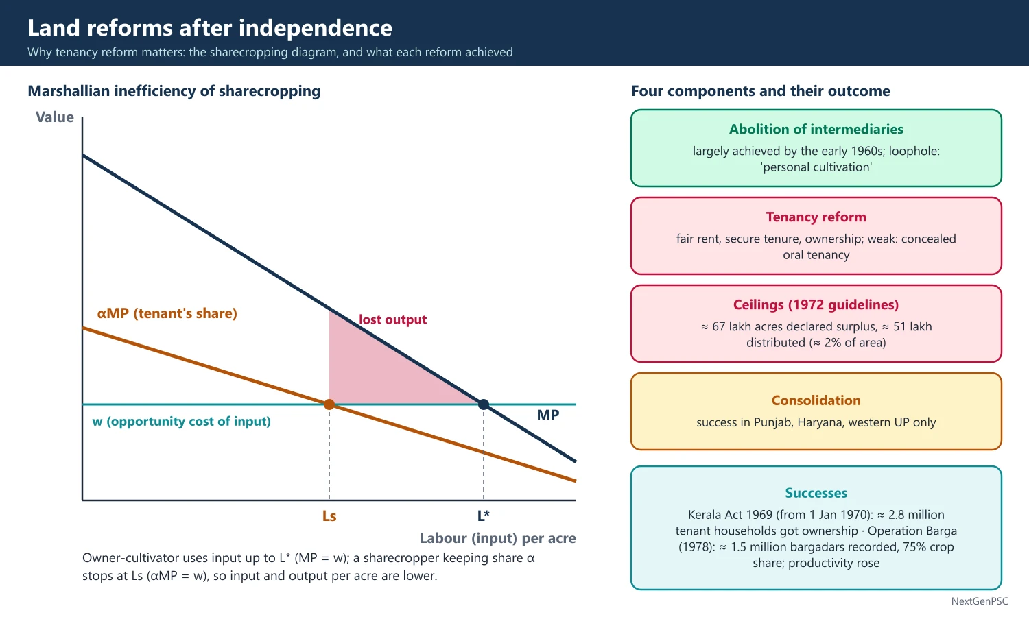
After 1947 India pursued land reforms in four parts: abolition of intermediaries (zamindari abolition, largely complete by the early 1960s), tenancy reform (regulating rent, security of tenure and ownership rights), ceilings on landholdings with redistribution of surplus land, and consolidation of holdings. Abolition of intermediaries succeeded widely, but tenancy and ceiling laws were weakly enforced except in states such as Kerala and West Bengal.
In simple words
Land reform means changing who owns and farms the land so that the person who tills it gets secure rights and a fair share; 'land to the tiller' was the slogan behind land reforms.
It is like giving a long-time tenant of a house the right to buy it, or at least protection from sudden eviction.
It matters because secure owners invest more and rural poverty falls.
UPSC asks you to assess the success and failure of land reforms and their effect on productivity and equity.
1. Objectives and Background
Inherited structure: colonial land systems left intermediaries, insecure tenants, sharecroppers paying half or more of the produce, fragmented holdings and very unequal ownership.
Congress Agrarian Reforms Committee (1949): chaired by J. C. Kumarappa, it recommended abolition of intermediaries, 'land to the tiller', ceilings, and cooperative farming; it set the agenda for the Plans.
Objectives (Planning Commission): remove impediments to agricultural production arising from the agrarian structure, and eliminate exploitation and social injustice within the agrarian system (paraphrase of plan documents).
Constitutional position: land is a State subject (Entry 18, State List), so laws were passed by states, with national guidelines from the Planning Commission and the Centre.
Constitutional amendments: the First Amendment (1951) inserted Articles 31A and 31B and the Ninth Schedule to protect land reform laws from challenge after the Kameshwar Singh case in Patna High Court; the Fourth (1955) and Seventeenth (1964) Amendments widened protection.
2. Abolition of Intermediaries
Laws: Uttar Pradesh Zamindari Abolition and Land Reforms Act (1950, in force 1952), Bihar Land Reforms Act (1950), Madhya Pradesh, Madras, West Bengal Estates Acquisition Act (1953) and others.
Results: by the early 1960s intermediaries were abolished in most states; tenants of intermediaries were brought into direct relation with the state; compensation was paid to zamindars, often in bonds.
Limits: zamindars could retain land under 'personal cultivation' (khudkasht, sir), a loophole that let many keep large areas and evict tenants to claim self-cultivation.
3. Tenancy Reforms
Three elements: regulation of rent (Planning Commission suggested rent not exceeding one-fourth to one-fifth of the produce), security of tenure (protection from eviction, with a right of resumption for the owner's personal cultivation in some states), and conferment of ownership rights on tenants.
Problems: most tenancies were oral and unrecorded; owners resumed land or converted tenants into 'labourers' or 'partners'; ejection rose before laws were passed; concealed tenancy became common.
Kerala: the Kerala Land Reforms (Amendment) Act, 1969, effective 1 January 1970, abolished tenancy and gave ownership to about 2.8 million tenant households according to estimates commonly cited, one of India's most thorough reforms.
West Bengal, Operation Barga (from 1978): a campaign to register sharecroppers (bargadars), giving them heritable tenure and a crop share of 75% (or 50% if the owner supplied inputs); about 1.5 million bargadars were recorded; Banerjee, Gertler and Ghatak (Journal of Political Economy, 2002) found that it raised agricultural productivity significantly, consistent with Marshallian sharecropping inefficiency.
Present stance: NITI Aayog's Model Agricultural Land Leasing Act (2016, prepared by an expert committee under T. Haque) argues that tenancy should be legalised and recorded so that tenants can get credit and owners lease without fear of losing land.
4. Ceilings on Landholdings
First phase (1950s–60s): ceilings were high, varied across states, applied to individuals rather than families, and had many exemptions (orchards, plantations, mechanised farms), so little land was declared surplus.
National guidelines (1972): family as the unit; ceilings of 10–18 acres for land with assured irrigation for two crops, 27 acres for land irrigated for one crop, and 54 acres for dry land; fewer exemptions; retrospective application to prevent evasive transfers.
Results: evasion through benami and fictitious transfers was widespread; Ministry of Rural Development data over the years show only about 67 lakh acres declared surplus and about 51 lakh acres distributed, around 2% of cultivated area (approximate figures).
Bhoodan and Gramdan: Vinoba Bhave's voluntary land-gift movement began at Pochampally (Telangana) on 18 April 1951; much donated land was poor or disputed and only part was distributed.
5. Consolidation of Holdings and Land Records
Consolidation: merging scattered plots into compact holdings; very successful in Punjab, Haryana and western Uttar Pradesh in the 1950s–60s, preparing the ground for tubewells and the Green Revolution; little progress in eastern and southern India.
Fragmentation trend: average operational holding fell from 2.28 hectares (1970–71) to 1.08 hectares (Agricultural Census 2015–16); in 2015–16 small and marginal holdings (below 2 hectares) were about 86% of holdings but about 47% of operated area.
Land records: the National Land Records Modernisation Programme (2008), restructured as the Digital India Land Records Modernisation Programme (2016), the 14-digit Unique Land Parcel Identification Number (ULPIN, 2021) and SVAMITVA (2020) for rural inhabited areas aim at conclusive titles.
6. Theory and Debates
Inverse farm size-productivity relationship: Farm Management Studies of the 1950s showed output per acre falling with farm size; Amartya Sen (1962, 1964) explained it through family labour applied up to a lower opportunity cost; Ashok Rudra, Krishna Bharadwaj and others debated it; it weakened in Green Revolution areas (debated).
Marshallian inefficiency of sharecropping: a tenant who keeps only a share of the output applies less effort or input than on owned land; Cheung (1969) argued that contracts could enforce efficient input levels; Operation Barga evidence supports the Marshallian view.
Poverty impact: Besley and Burgess (Quarterly Journal of Economics, 2000) found that land reform legislation, especially tenancy reform and abolition of intermediaries, reduced rural poverty across Indian states, though some measures had weak or negative associations with output.
Mode of production debate (1970s, Economic and Political Weekly): Utsa Patnaik, Ashok Rudra, Amit Bhaduri and others debated whether Indian agriculture was semi-feudal or capitalist, with implications for whether land reform or technology would drive growth.
East Asian contrast: Japan, South Korea and Taiwan carried out thorough land-to-the-tiller reforms (late 1940s–early 1950s) that created egalitarian smallholder agriculture and supported industrial growth; India's reforms were less thorough because of political power of landed groups.
7. Diagrams and Charts
Marshallian sharecropping diagram: x-axis labour (or input) per acre, y-axis value; draw the marginal product curve MP and a lower curve αMP for the tenant's share α; the wage line w cuts MP at L* (efficient) and αMP at Ls (sharecropper), showing under-use of input Ls below L*; shade the lost output.
Inverse relationship sketch: x-axis farm size, y-axis output per acre; a downward-sloping curve.
Holding structure chart: bar chart comparing the share of holdings and share of area for marginal, small, semi-medium, medium and large holdings (Agricultural Census 2015–16).
8. Recent Issues
Concealed tenancy today: official surveys record only a small share of operated land as leased in, but actual tenancy, mostly oral, is believed to be much larger, which keeps tenants out of institutional credit, insurance and support schemes.
Recognising tenants: the Andhra Pradesh Land Licensed Cultivators Act (2011) and the Andhra Pradesh Crop Cultivator Rights Act (2019) give tenants cultivator cards for credit and benefits without affecting ownership, an approach close to the 2016 model Act.
Women's land rights: the Hindu Succession (Amendment) Act, 2005, gave daughters equal coparcenary rights; Bina Agarwal's A Field of One's Own (1994) argued that women's ownership of land improves welfare and bargaining power.
Landlessness: the Socio-Economic and Caste Census (2011) found that about 56% of rural households owned no land, showing how limited redistribution was.
Land acquisition: the Right to Fair Compensation and Transparency in Land Acquisition, Rehabilitation and Resettlement Act, 2013, replaced the Land Acquisition Act, 1894, raising compensation and requiring consent and social impact assessment for many projects.
9. Using It in the Exam
10 marks: components of land reform and one success (Kerala or Operation Barga).
15 marks: why ceiling and tenancy laws failed in most states.
20 marks: objectives, components, achievements and failures, evidence on productivity and poverty (Banerjee-Gertler-Ghatak, Besley-Burgess), present agenda (leasing law, land records).
Keywords: land to the tiller, intermediaries, resumption, concealed tenancy, benami, ceiling, consolidation, inverse relationship, Marshallian inefficiency, ULPIN.
| Component | Aim | Outcome | Best example |
|---|---|---|---|
| Abolition of intermediaries | Direct link between state and cultivator | Largely achieved by early 1960s | Uttar Pradesh, Bihar Acts (1950) |
| Tenancy reform | Fair rent, secure tenure, ownership | Weak; concealed tenancy spread | Kerala (1969 Act), Operation Barga (1978) |
| Ceilings | Redistribute surplus land | Small area declared and distributed | 1972 national guidelines |
| Consolidation | Compact holdings for efficiency | Success in north-west only | Punjab, Haryana |
| Land records | Clear titles, credit access | Ongoing digitisation | DILRMP (2016), ULPIN (2021) |
Mains points
- Structure answers around the four components and judge each separately; examiners penalise blanket statements.
- Give the constitutional context (State subject, First Amendment and Ninth Schedule).
- Use Kerala and Operation Barga as successes, with the Banerjee-Gertler-Ghatak finding on productivity.
- Explain failure through political economy: landed interests, unrecorded tenancy, benami transfers, weak administration.
- Bring in theory: the inverse relationship (Sen) and Marshallian sharecropping inefficiency, with the diagram.
- Link to the present: holding fragmentation (1.08 hectares in 2015–16), leasing reform (2016 model Act) and digitised land records.
Did you know?
- The Ninth Schedule began with 13 laws in 1951, almost all of them land reform Acts; it now lists over 280 laws.
Green Revolution: Strategy, Gains and Problems
The Green Revolution (from 1965–66) combined high-yielding varieties of wheat and rice with assured irrigation, chemical fertilisers and pesticides, supported by minimum support prices, procurement by the Food Corporation of India and institutional credit. It made India self-sufficient in food grains, but gains were concentrated in wheat and rice and in irrigated regions such as Punjab, Haryana and western Uttar Pradesh, with later problems of groundwater depletion, soil degradation and inequality.
In simple words
The Green Revolution was a jump in farm output in the late 1960s when farmers used new short, high-yielding wheat and rice seeds with water, fertiliser and assured prices; these are high-yielding varieties.
It is like upgrading from an old engine to a powerful new one, which needs better fuel (water and fertiliser) to run.
It ended India's dependence on food imports but helped some regions and crops far more than others and strained water and soil.
UPSC asks you to assess its strategy, gains and problems.
1. Background
Food crisis: slow growth of food output, droughts in 1965–66 and 1966–67, and dependence on US wheat under PL-480 (the 'ship-to-mouth' existence) made food self-sufficiency a political priority.
Earlier programmes: the Intensive Agricultural District Programme (IADP, 1960–61, a 'package' approach in selected districts) and the Intensive Agricultural Area Programme (IAAP, 1964) showed the value of combined inputs.
Science: Norman Borlaug's semi-dwarf wheat varieties from CIMMYT in Mexico (such as Lerma Rojo 64 and Sonora 64) and IRRI's IR8 rice (1966) responded strongly to fertiliser and irrigation without lodging; M. S. Swaminathan led adaptation and testing in India; Borlaug received the Nobel Peace Prize in 1970.
Political leadership: C. Subramaniam, Union Agriculture Minister (1964–67), with B. Sivaraman, pushed the New Agricultural Strategy, supported by Lal Bahadur Shastri and Indira Gandhi.
2. The Strategy Step by Step
High Yielding Varieties Programme (HYVP, kharif 1966–67): concentrated HYV seeds, fertiliser, pesticides and credit in areas with assured irrigation.
Price support: the Agricultural Prices Commission (1965; renamed Commission for Agricultural Costs and Prices in 1985) recommended minimum support prices to make the new technology profitable and reduce price risk.
Procurement and distribution: the Food Corporation of India (set up in January 1965 under the Food Corporations Act, 1964) procured grain at MSP, built buffer stocks and supplied the public distribution system.
Inputs and infrastructure: expansion of fertiliser production and imports, subsidised power for tubewells, canal irrigation, rural electrification, agricultural universities (Pantnagar 1960, Punjab Agricultural University 1962) and extension services.
Credit: cooperative credit and, after bank nationalisation (1969), commercial bank lending to agriculture under priority-sector norms.
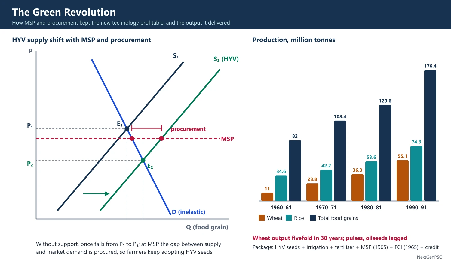
Economic logic: technical change shifted the production function upward and the supply curve to the right; MSP provided a floor so that farmers captured enough of the gains to keep adopting, avoiding the price collapse a bigger harvest would otherwise cause with inelastic demand.
3. Gains
Output: wheat production rose from about 11 million tonnes (1960–61) to about 24 million tonnes (1970–71), 36 million tonnes (1980–81) and 55 million tonnes (1990–91); total food grains rose from about 82 million tonnes (1960–61) to about 176 million tonnes (1990–91) (Ministry of Agriculture data).
Food security: PL-480 imports ended by the early 1970s; buffer stocks allowed the PDS to expand and protected against droughts (for example 1987); food grain output exceeded 350 million tonnes in 2024–25 (Ministry of Agriculture estimates), making India a major rice exporter.
Incomes and employment: higher farm incomes in adopting regions; demand for labour rose initially with multiple cropping; rural non-farm activity expanded through linkages (Hazell and Ramasamy, The Green Revolution Reconsidered, 1991, on North Arcot).
Prices and poverty: lower real food prices helped the urban and rural poor; rural poverty fell from the mid-1970s.
4. Problems
Crop bias: gains were largest in wheat, then rice; pulses, oilseeds and coarse cereals lagged, leading later to the Technology Mission on Oilseeds (1986) and continuing pulse imports.
Regional inequality: concentrated in irrigated north-west India (Punjab, Haryana, western Uttar Pradesh) and some southern deltas; rainfed eastern and central India gained little until later; the Bringing Green Revolution to Eastern India programme (BGREI, 2010–11) addressed this.
Inter-personal inequality: early studies (Francine Frankel, India's Green Revolution: Economic Gains and Political Costs, 1971) found that larger farmers gained more and tenants were evicted; later studies found small farmers adopted with a lag and benefited (G. S. Bhalla and G. K. Chadha on Punjab); the net effect is debated.
Mechanisation and labour: tractors and later combine harvesters displaced some labour; migrant labour from Bihar and eastern Uttar Pradesh met peak demand in Punjab.
Environment: over-extraction of groundwater (Punjab's groundwater draft well above 100% of annual recharge in most blocks, Central Ground Water Board assessments), soil nutrient imbalance (urea-heavy use against the recommended NPK ratio of about 4:2:1), salinity and waterlogging in canal areas, pesticide residues, and stubble burning.
Fiscal burden: fertiliser, power and water subsidies and open-ended procurement grew large and crowded out public investment (Gulati and Narayanan, The Subsidy Syndrome in Indian Agriculture, 2003).
Stagnation: yield growth slowed after the mid-1980s and especially in the 1990s, as the technology package reached its limits and public investment declined.
5. Diagrams to Draw
Supply shift with MSP: x-axis quantity of food grain, y-axis price; draw a steep (inelastic) demand curve and supply curve S1; HYV technology shifts supply to S2; without support, price falls sharply from P1 to P2; draw a horizontal MSP line above P2 showing that government procurement absorbs the excess and maintains farmer incentives; mark procurement quantity as the gap between supply and market demand at MSP.
Production function shift: x-axis fertiliser per hectare, y-axis yield; the traditional variety's curve flattens early; the HYV curve rises higher and responds to more fertiliser, showing complementarity with inputs.
Output trend chart: wheat, rice and pulses production from 1960–61 to 1990–91 showing rapid wheat growth and flat pulses.
6. Theory and Debates
Induced innovation (Hayami and Ruttan, Agricultural Development: An International Perspective, 1971): land-scarce countries develop land-saving biological and chemical technology; the Green Revolution fits this pattern.
Schultz's argument (1964): traditional farmers are efficient but poor; growth comes from new, profitable inputs; adoption of HYVs by Indian farmers confirmed their responsiveness to profit.
Red revolution debate: some predicted that the Green Revolution would turn red through class conflict (a phrase associated with commentators in the late 1960s); widespread revolt did not occur, though agrarian conflict rose in some regions.
Sustainability critique: Vandana Shiva (The Violence of the Green Revolution, 1991) and others criticised its ecological and social costs; supporters reply that without it India would have needed far more land and imports.
7. Spread and Later Policy
Spread in the 1980s: the technology later spread to rice in eastern and southern states such as West Bengal, Andhra Pradesh and Tamil Nadu, helped by private tubewells and power, narrowing regional gaps in rice.
Operation Flood (from 1970): the National Dairy Development Board under Verghese Kurien built a cooperative milk grid on the Anand model, the 'White Revolution', making India the world's largest milk producer.
National Food Security Mission and RKVY (2007): launched to raise output of rice, wheat and pulses in lagging districts and to give states flexible funds for agriculture.
Crop diversification: programmes since 2013–14 in Punjab, Haryana and western Uttar Pradesh pay farmers to shift area from paddy to maize, pulses and oilseeds to save groundwater.
Food security link: the National Food Security Act (2013) and free grain under the Pradhan Mantri Garib Kalyan Anna Yojana (extended for five years from 1 January 2024) depend on the procurement system built during the Green Revolution.
8. Using It in the Exam
10 marks: components of the New Agricultural Strategy (HYV, irrigation, fertiliser, MSP, FCI, credit).
15 marks: gains and problems with output data and years.
20 marks: strategy, institutional support, gains, crop, regional, personal and environmental problems, and lessons for a second Green Revolution (rainfed areas, pulses, water-use efficiency).
Keywords: HYV, package approach, IADP, MSP, FCI, buffer stock, crop bias, regional disparity, groundwater depletion, induced innovation, second-generation problems.
Attributed idea: Swaminathan warned as early as 1968 that intensive cultivation without care for soil, water and ecology could lead to agricultural disaster rather than prosperity, and later called for an evergreen revolution that raises yields without ecological harm (paraphrase).
| Year | Wheat | Rice | Total food grains |
|---|---|---|---|
| 1960–61 | 11.0 | 34.6 | 82.0 |
| 1970–71 | 23.8 | 42.2 | 108.4 |
| 1980–81 | 36.3 | 53.6 | 129.6 |
| 1990–91 | 55.1 | 74.3 | 176.4 |
Mains points
- Present the Green Revolution as a package (seeds, water, fertiliser, prices, procurement, credit), not just new seeds.
- Use production data with years to show gains; note the crop bias with pulses and oilseeds.
- Discuss the inequality debate fairly: Frankel's early pessimism versus later evidence of small-farmer adoption.
- Explain environmental problems with specific examples (Punjab groundwater, NPK imbalance, stubble burning).
- Draw the supply-shift diagram with an MSP floor; it shows why price support was integral.
- Conclude with lessons for rainfed areas, crop diversification and water-use efficiency (BGREI, micro-irrigation).
Did you know?
- The term 'Green Revolution' was coined by William Gaud of USAID in a speech in March 1968.
Capital Formation and Institutional Credit in Agriculture
Capital formation in agriculture (irrigation, land development, machinery, livestock, orchards) drives long-run farm growth. Public investment rose until about 1980 and then fell as input subsidies grew, while private investment by farmers became dominant. Institutional credit replaced moneylenders through cooperatives, bank nationalisation (1969), priority-sector lending, Regional Rural Banks (1975) and NABARD (1982), though small and tenant farmers remained underserved.
In simple words
Capital formation in agriculture means building things that raise farm output for years: wells, canals, levelled fields, tractors and orchards; this is capital formation.
Institutional credit means loans from banks and cooperatives instead of moneylenders, like replacing a costly local lender with a fair bank loan.
Both matter because farmers cannot invest without credit, and low investment keeps yields low.
UPSC asks about trends in public and private investment, subsidies versus investment, and how rural credit institutions developed.
1. Concepts and Definitions
Gross capital formation (GCF) in agriculture: addition to fixed assets (irrigation works, wells and tubewells, land improvement, farm machinery, farm buildings, livestock, orchards and plantations) plus change in stocks; usually measured as a share of agricultural GDP or GVA.
Public versus private: public GCF is mainly major and medium irrigation, flood control, rural electrification and research; private GCF is mainly farmers' investment in tubewells, pumps, tractors, land levelling and livestock.
Investment in agriculture versus for agriculture: investment in agriculture is GCF within the sector; investment for agriculture includes rural roads, power, markets, research and storage outside the sector's accounts but essential to it.
Institutional credit: loans from cooperatives, commercial banks, regional rural banks and other formal lenders, as distinct from non-institutional credit from moneylenders, traders, landlords and relatives.
2. Trends in Capital Formation (Pre-liberalisation)
1950s–1970s: heavy public investment in irrigation (Bhakra-Nangal, Hirakud, Damodar Valley, Nagarjuna Sagar) and electrification; public investment was close to half of total agricultural investment around 1980.
1980s decline: public GCF in agriculture fell in real terms from about 1980–81 as governments spent more on subsidies (fertiliser, power, irrigation water, credit) and salaries; private investment, especially in tubewells, continued to rise.
Subsidy versus investment trade-off: Gulati and Narayanan (2003) and others showed that input subsidies rose while public investment fell, and that returns to investment in research, roads and irrigation were much higher than returns to subsidies (Fan, Gulati and Thorat, IFPRI studies, 2000s).
Complementarity debate: some studies (for example Mishra and Chand, 1995) found that public investment crowds in private investment by providing irrigation and power; others found weaker or mixed effects; the relationship is debated.
Recent data: the Economic Survey 2023–24 reported that GCF in agriculture as a share of agricultural GVA rose from 17.7% in 2021–22 to 19.9% in 2022–23, driven partly by higher public investment, but average real growth of agricultural GCF was below the rate needed for the goal of doubling farmers' incomes.
3. Institutional Credit: Evolution
All-India Rural Credit Survey (1951–54): the committee chaired by A. D. Gorwala found that moneylenders supplied about 70% of rural credit, cooperatives about 3% and commercial banks about 1%; its conclusion was that cooperation had failed but cooperation must succeed (paraphrase); it recommended an integrated scheme of rural credit with state partnership in cooperatives and the creation of the State Bank of India (1955).
Cooperatives: a three-tier short-term structure (primary agricultural credit societies at village level, district central cooperative banks, state cooperative banks) and a long-term structure (land development banks); problems included elite capture, poor recovery and politicisation.
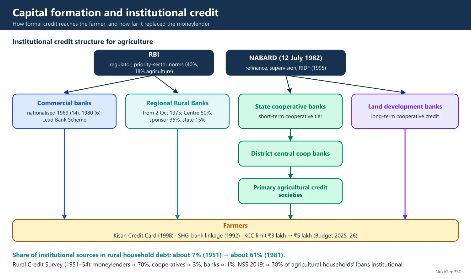
Social control and nationalisation: social control of banks (1968) and nationalisation of 14 major banks (19 July 1969), with six more in 1980, extended branches to rural areas; the Lead Bank Scheme (1969) gave each district a lead bank.
Priority-sector lending: formalised in 1972; targets later fixed at 40% of net bank credit for priority sectors, with 18% for agriculture (sub-targets for small and marginal farmers added later).
Regional Rural Banks: recommended by the Narasimham Working Group (1975); the first five were set up on 2 October 1975, and the Regional Rural Banks Act was passed in 1976; jointly owned by the Centre (50%), sponsor bank (35%) and state (15%), they combined local feel with commercial discipline.
NABARD: set up on 12 July 1982 on the recommendation of the Committee to Review Arrangements for Institutional Credit for Agriculture and Rural Development (CRAFICARD, chaired by B. Sivaraman, 1979–81); it refinances cooperatives, RRBs and banks, supervises cooperatives and RRBs, and manages the Rural Infrastructure Development Fund (1995).
Integrated Rural Development Programme (1978–80 onward): subsidised bank loans for assets to the rural poor; it suffered from poor targeting and defaults.
Loan waiver of 1990: the Agricultural and Rural Debt Relief Scheme (1990) waived loans up to Rs 10,000, which the Narasimham Committee (1991) and others argued damaged credit discipline.
4. Results and Problems
Rising institutional share: All-India Debt and Investment Surveys show the share of institutional sources in rural household debt rising from about 7% in 1951 to about 61% in 1981, after which it stagnated through the 1990s; non-institutional sources regained some ground in the 1990s and early 2000s.
Persisting gaps: tenant farmers and sharecroppers without land titles, small and marginal farmers and eastern states received less credit; moneylenders remained important for consumption and emergency loans.
Problems of directed credit: by 1990 rural banking had high costs, low recovery, weak cooperatives and politically driven waivers; the Narasimham Committee (1991) recommended phasing down directed credit and interest controls, and the Khusro Committee (1989) reviewed agricultural credit.
Later steps: Kisan Credit Card (1998, on the R. V. Gupta Committee's recommendation), Self-Help Group-Bank Linkage (from 1992, piloted by NABARD), interest subvention for short-term crop loans, and the raising of the KCC loan limit under the Modified Interest Subvention Scheme from Rs 3 lakh to Rs 5 lakh in the Union Budget 2025–26.
Current position: NSS 77th round (2019) found that about 70% of outstanding loans of agricultural households came from institutional sources, so about 30% still came from non-institutional sources.
5. Diagrams to Draw
Public versus private GCF trend: x-axis time (1960–2000), y-axis share of agricultural GDP; draw public GCF rising until about 1980 and then falling, private GCF rising steadily, with subsidies rising sharply after 1980.
Credit structure chart: RBI and NABARD at top → commercial banks, RRBs, state cooperative banks → district central cooperative banks → primary agricultural credit societies → farmers; separate line for land development banks (long-term credit).
Dual credit market: x-axis quantity of credit, y-axis interest rate; formal rate rf low with rationed supply (vertical at the bank's limit) and informal rate ri high; borrowers excluded from formal credit pay ri.
6. Theory and Debates
Why rural credit markets fail: information asymmetry, lack of collateral, high transaction costs, covariant risk (whole villages hit by drought) and enforcement problems (Stiglitz and Weiss, 'Credit Rationing in Markets with Imperfect Information', 1981); moneylenders use personal information and interlinked contracts (credit tied to labour or crop sales).
Interlinked markets: Amit Bhaduri (1973) argued that landlords as lenders could profit from keeping tenants indebted and may resist productivity-raising innovations; Bardhan (1980s) analysed interlinked contracts more generally.
Supply-leading finance: Hugh Patrick (1966) argued that creating financial institutions ahead of demand can promote development, a rationale for India's rural branch expansion; Burgess and Pande (American Economic Review, 2005) found that the rural branch expansion rule of 1977–1990 reduced rural poverty, a finding later debated.
7. Capital Formation after Liberalisation
Agriculture Infrastructure Fund (2020): a ₹1 lakh crore financing facility with interest subvention for post-harvest infrastructure such as warehouses, cold chains and processing units.
Irrigation investment: the Pradhan Mantri Krishi Sinchayee Yojana (2015), with its 'Per Drop More Crop' micro-irrigation component, and NABARD's Long Term Irrigation Fund (2016–17) target unfinished irrigation projects.
Rural Infrastructure Development Fund (1995–96): funded from banks' shortfalls in priority-sector lending and managed by NABARD, it finances state projects in irrigation, rural roads and bridges.
Income support versus investment: PM-KISAN (February 2019) pays ₹6,000 a year to landholding farmers; critics argue that such transfers compete with public investment, while supporters note they ease liquidity for inputs (debated).
Risk and investment: crop insurance under the Pradhan Mantri Fasal Bima Yojana (2016) aims to reduce income risk, which otherwise discourages farmers from borrowing to invest.
Mechanisation: India has become one of the world's largest tractor markets, and custom hiring centres for small farmers have been promoted since the mid-2010s.
8. Using It in the Exam
10 marks: reasons for the fall in public investment in agriculture after 1980, or the role of NABARD.
15 marks: evolution of institutional credit from the Rural Credit Survey to RRBs and NABARD.
20 marks: trends in capital formation (public, private, subsidies), institutional credit evolution and results, persisting gaps and reforms, with data and years.
Keywords: GCF in agriculture, crowding in, subsidy syndrome, integrated scheme of rural credit, priority sector, RRB, NABARD, interlinked markets, credit rationing, supply-leading finance.
| Year | Institution or measure | Significance |
|---|---|---|
| 1904 | Cooperative Credit Societies Act | Start of cooperative credit |
| 1954 | All-India Rural Credit Survey (Gorwala) | Moneylenders about 70% of rural credit; integrated scheme proposed |
| 1955 | State Bank of India | Rural branch expansion of a state-owned bank |
| 1969 | Nationalisation of 14 banks; Lead Bank Scheme | Credit directed to agriculture and rural areas |
| 1975–76 | Regional Rural Banks | Local, low-cost rural banking |
| 1982 | NABARD | Apex refinance and development bank for agriculture |
| 1998 | Kisan Credit Card | Flexible short-term crop credit |
Mains points
- Distinguish public and private capital formation and investment in versus for agriculture.
- Explain the post-1980 fall in public investment through the subsidy-investment trade-off, with evidence on returns (IFPRI studies).
- Trace institutional credit in a timeline from the Rural Credit Survey to NABARD, with dates and committees.
- Use the AIDIS figures (institutional share about 7% in 1951 to about 61% in 1981) to show progress and its later stagnation.
- Bring in theory: credit rationing (Stiglitz-Weiss), interlinked markets (Bhaduri) and supply-leading finance (Patrick, Burgess-Pande).
- Common mistake: treating a rise in credit volume as proof of better access; distribution by farm size, tenancy and region matters.
Did you know?
- The first five Regional Rural Banks opened on Gandhi Jayanti, 2 October 1975, including Prathama Bank in Moradabad, Uttar Pradesh.
UPSC Previous Year Questions: Agriculture before Liberalisation
From 2014 to 2026 UPSC asked 23 question parts worth 355 marks from this chapter in Paper II. The Green Revolution (10 parts) and land reforms (8 parts) dominate, followed by capital formation and institutional credit in agriculture (5). Every question below has a model answer written to the UPSC word limit.
In simple words
Read the question and write your own answer in the time limit first: about 7 minutes for 10 marks and 11 minutes for 15 or 20 marks.
Then compare it with the model answer: did you give output figures with years, name the scheme, committee or study, and present both sides?
Note what you missed, revise that topic in the notes above, and rewrite the answer after a few days.
1. Land Reforms and Land Tenure after Independence
Example 1 (UPSC 2026, 10 marks): Assess the efficacy of land tenurial system reforms in post-Independent India in addressing intermediary abolition.
Paper and question: Paper II, Q1(c)
Approach: Explain how intermediaries were abolished (laws, constitutional amendments), assess its efficacy (what it achieved and where it fell short), and conclude.
Abolition of intermediaries (zamindars, jagirdars, inamdars) was the first and most successful plank of post-independence land reform, recommended by the Congress Agrarian Reforms Committee under J.C. Kumarappa (1949).
Process: states passed laws such as the Uttar Pradesh Zamindari Abolition and Land Reforms Act (1950, in force 1952), the Bihar Land Reforms Act (1950) and the West Bengal Estates Acquisition Act (1953); the First Amendment (1951) added Articles 31A and 31B and the Ninth Schedule to protect them from court challenges.
Efficacy: by the early 1960s intermediary rights were abolished in most states, bringing about 2 crore tenants into direct contact with the state and ending the zamindari revenue system.
Shortcomings: zamindars kept large 'personal cultivation' (khudkasht) land, evicted tenants by claiming self-cultivation, received compensation, and many became large landowners; sub-tenants and sharecroppers often gained nothing.
Hence the reform abolished a feudal class legally but redistributed less land than hoped.
Example 2 (UPSC 2026, 20 marks): Evaluate the success of land reforms in post-Independent India. Why was the success limited in certain States while non-existent in others? Link land reforms to the broader agricultural transformation and explain.
Paper and question: Paper II, Q2(a)
Approach: Evaluate each component (intermediary abolition, tenancy reform, ceilings, consolidation), explain why success varied across states (political will, records, mobilisation), then link land reform to agricultural transformation.
Land reforms after 1947 aimed at 'land to the tiller', equity and higher productivity, through four components.
Success by component: (i) abolition of intermediaries was largely achieved by the early 1960s; (ii) tenancy reform (security, fair rent, ownership) was weak, as oral leases, evictions and 'voluntary surrenders' defeated it; (iii) ceilings produced only about 67 lakh acres declared surplus and about 51 lakh acres distributed, roughly 2% of cultivated area, due to benami transfers and exemptions; (iv) consolidation succeeded in Punjab, Haryana and western Uttar Pradesh but barely elsewhere.
Why success varied: Kerala (Land Reforms Amendment Act, 1969, effective 1970) abolished tenancy and gave ownership to millions of tenants; West Bengal's Operation Barga (from 1978) recorded about 15 lakh sharecroppers. Both had strong political will, peasant mobilisation and left-wing governments. In Bihar and much of the Hindi belt, landlords dominated politics and administration, land records were poor and tenants were socially weak, so reforms remained on paper.
Link to agricultural transformation: where reforms gave secure rights, investment and productivity rose: Banerjee, Gertler and Ghatak (2002) attribute a significant part of West Bengal's agricultural growth in the 1980s to Operation Barga. Consolidation in Punjab paved the way for tubewells and the Green Revolution. Besley and Burgess (2000) found that land reform reduced rural poverty across states. Where reforms failed, insecure tenancy and fragmented holdings held back investment, mechanisation and credit.
Today: average holdings fell to 1.08 hectares (Agriculture Census 2015–16), so the agenda has shifted to tenancy legalisation (NITI Model Land Leasing Act, 2016), digital land records and women's land rights.
Thus land reform succeeded where politics backed it, and it was a foundation for, not a substitute for, technological transformation.
Example 3 (UPSC 2025, 20 marks): Is land reform necessary to improve agricultural productivity in India? Discuss.
Paper and question: Paper II, Q2(a)
Approach: Argue that land reform is necessary (security, incentives, inverse farm-size relation, credit, consolidation) but not sufficient, with Indian evidence, and suggest a current reform agenda.
Agricultural productivity depends on technology, inputs and institutions; land reform shapes the institutional base: who owns, operates and invests in land.
Why land reform is necessary: (i) security and incentives: under sharecropping a tenant keeps only part of the output, causing Marshallian inefficiency; Operation Barga in West Bengal (from 1978), which gave sharecroppers secure tenure and a 75% share, raised productivity substantially (Banerjee, Gertler and Ghatak, 2002); (ii) inverse farm size-productivity relation: Farm Management Studies of the 1950s and Amartya Sen (1962) showed small family farms produce more per acre, so redistribution need not reduce output; (iii) credit: recorded ownership or tenancy allows access to bank credit, insurance and subsidies; (iv) consolidation of fragmented plots enables tubewells and mechanisation, as in Punjab before the Green Revolution.
Not sufficient: holdings averaging 1.08 hectares (Agriculture Census 2015–16) cannot be made more productive by redistribution alone; irrigation, seeds, research, markets and credit are also needed.
Current agenda: legalise and record tenancy (NITI Aayog's Model Agricultural Land Leasing Act, 2016), digitise land records (DILRMP, ULPIN), promote farmer producer organisations to overcome small scale, and secure women's land rights.
Evidence from states: Kerala and West Bengal, which implemented tenancy reform most thoroughly, saw secure cultivators invest in their land, while in Bihar insecure, unrecorded sharecropping kept investment and yields low. Besley and Burgess (2000) found that tenancy reform and abolition of intermediaries reduced rural poverty across Indian states, and East Asian land reforms show that secure smallholders adopt new technology quickly.
So land reform is necessary for productivity but must be combined with technology and market reforms.
Example 4 (UPSC 2023, 15 marks): Explain the concept of ceiling on agricultural landholding in India. Examine its rationality with respect to equity and efficiency.
Paper and question: Paper II, Q3(c)
Approach: Explain the concept and evolution of land ceilings (1950s laws, 1972 guidelines), then examine its rationale for equity and for efficiency (inverse relation vs scale economies), with results and a conclusion.
A land ceiling is the legal maximum area of agricultural land a person or family may own; land above it is declared surplus, acquired by the state and distributed to the landless and marginal farmers.
Evolution: first-phase laws in the 1950s and 1960s set high ceilings on individuals with many exemptions; the national guidelines of 1972 made the family the unit and lowered ceilings to about 10–18 acres for land with assured irrigation for two crops, 27 acres for single-crop irrigated land and 54 acres for dry land.
Equity rationale: India's land was highly concentrated, and land is the main source of rural income, status and credit; redistributing surplus land reduces asset inequality and poverty.
Efficiency rationale: the inverse relation between farm size and output per acre (Farm Management Studies; Amartya Sen, 1962) implies that small family farms use land more intensively, so redistribution can raise total output. Against this, large farms enjoy scale economies in machinery, credit and marketing, and very small plots may be unviable; the efficiency argument is debated.
Results: only about 67 lakh acres were declared surplus and about 51 lakh acres distributed, around 2% of cultivated area, because of benami transfers, litigation and weak enforcement.
Ceilings were rational for equity and broadly consistent with efficiency, but poor implementation limited their impact.
Example 5 (UPSC 2021, 20 marks): Do you think that effective land reforms are necessary but not sufficient conditions for raising agricultural productivity in India? Explain your answer.
Paper and question: Paper II, Q3(a)
Approach: Agree: explain why land reforms are necessary (incentives, security, credit, inverse relation) and why not sufficient (technology, irrigation, markets, credit, extension), using Indian evidence, and conclude.
Yes. Land reforms create the institutional conditions for productivity, but productivity also needs technology and infrastructure.
Necessary because: (i) incentives: secure owner-cultivators invest in land improvement, while insecure sharecroppers under-invest (Marshallian inefficiency); Operation Barga (West Bengal, 1978 onward) raised productivity, as Banerjee, Gertler and Ghatak (2002) showed; (ii) access to credit and inputs: recorded rights allow bank credit, insurance and subsidies; (iii) inverse farm size-productivity relation: small family farms use labour intensively, so redistribution can raise output; (iv) consolidation enabled tubewells and mechanisation in Punjab and Haryana; (v) less inequality strengthens rural demand and reduces conflict.
Not sufficient because: productivity jumped mainly with the Green Revolution package of high-yielding seeds, fertiliser, irrigation, credit and assured prices after 1966, in regions with and without thorough land reforms; Kerala, despite the most complete reform, did not see a matching rise in food output, as cropping shifted and holdings were tiny; markets, extension, research, roads and storage are equally important.
Evidence of complementarity: East Asian land reforms (Japan, Taiwan, South Korea) succeeded because they were combined with irrigation, research and credit.
Today: with average holdings of about 1.08 hectares (2015–16), the emphasis has moved to tenancy legalisation (Model Land Leasing Act, 2016), land records digitisation and farmer producer organisations.
Hence land reform is a necessary but not a sufficient condition for higher agricultural productivity.
Example 6 (UPSC 2019, 20 marks): "The progress in the implementation of tenancy and revenue reforms during the first three decades after independence in India was not satisfactory." Do you agree with this view? Do you think that the advent of the Green Revolution made such land reforms policy redundant?
Paper and question: Paper II, Q3(a)
Approach: Agree with the first view (evidence on tenancy and revenue reforms 1950–80 and reasons for failure); then answer the second part: the Green Revolution did not make land reform redundant, giving reasons.
Yes, apart from the abolition of intermediaries, tenancy and revenue reforms in 1950–80 made unsatisfactory progress.
Tenancy reforms: laws provided security of tenure, regulation of rent (generally one-fourth to one-fifth of produce, as the Plans suggested) and ownership rights for tenants. In practice, most tenancies were oral and unrecorded; landlords evicted tenants by claiming 'personal cultivation' or forcing 'voluntary surrenders'; rents stayed at about half the crop; tenancy went underground as concealed sharecropping. Only Kerala (1969–70) and later West Bengal's Operation Barga (1978) achieved substantial results.
Revenue reforms: land revenue, once the main tax, was kept low and stagnant after independence, losing its role in mobilising agricultural surplus; proposals for progressive agricultural taxation (such as the Raj Committee on agricultural taxation, 1972) were not implemented.
Reasons: landlord dominance in state politics and administration, poor land records, lack of peasant organisation, legal loopholes and delays, and the low priority given to reform once the Green Revolution began.
Did the Green Revolution make land reform redundant? No. (i) Its gains went disproportionately to larger farmers with irrigation and credit, so land concentration mattered more, not less; (ii) insecure tenants could not afford or risk new inputs; (iii) secure rights were needed for credit and investment in tubewells; (iv) Operation Barga showed that tenancy reform could raise productivity even after the Green Revolution; (v) the Green Revolution itself relied on earlier consolidation in Punjab.
Diagram: share of holdings and share of operated area by size class (marginal, small, medium, large) as paired bars, showing that marginal holdings are numerous but hold a small share of area.
Hence land reform and technology are complements; the Green Revolution increased the need for secure and equitable land rights.
Example 7 (UPSC 2018, 15 marks): How would you justify the policy of land reforms in the light of the farm size-productivity debate in India?
Paper and question: Paper II, Q3(b)
Approach: Explain the farm size-productivity debate (inverse relation, its explanations, its weakening after the Green Revolution), then use it to justify land reforms, with caveats.
The farm size-productivity debate began with the Farm Management Studies of the 1950s, which found that output per acre fell as farm size rose: the inverse relationship.
Explanations: (i) Amartya Sen (1962, 1964) argued that small family farms apply labour up to the point where its marginal product equals the low opportunity cost of family labour, while large farms hire labour at the market wage and use less; (ii) small farms crop more intensively and irrigate more of their land; (iii) differences in land quality, since small farms may be on better land (A.K. Bhattacharya, Rudra).
Debate: Ashok Rudra, Utsa Patnaik and others questioned the generality of the relation; after the Green Revolution, larger farms with better access to irrigation, credit and machinery raised yields, and several studies found the inverse relation weakened or disappeared in advanced regions such as Punjab.
Justification for land reform: if small farms are at least as productive per acre, redistributing land from large to small holders does not reduce output and may raise it, while improving equity and employment; tenancy security also removes the Marshallian disincentive of sharecropping, as Operation Barga showed.
Caveats: holdings must not be too small to use modern inputs; small farmers need credit, irrigation and markets, and producer organisations to capture scale economies. Thus the debate supports land reform combined with support services.
Example 8 (UPSC 2014, 15 marks): Why are land reforms still not complete in India? What are the obstacles in its way? Elaborate.
Paper and question: Paper II, Q2(c)
Approach: Explain why land reforms remain incomplete and elaborate the obstacles (political, administrative, legal, social, economic), with examples, and suggest the way forward.
Beyond abolishing intermediaries, India's land reforms remain incomplete: ceilings redistributed only about 2% of cultivated area, tenancy is largely unrecorded, and about 56% of rural households owned no land (SECC, 2011).
Political obstacles: landowning classes dominated state legislatures and parties; land is a state subject, so political will varied, and only Kerala and West Bengal pushed reforms hard.
Administrative obstacles: outdated and incomplete land records, unrecorded oral tenancies, and a revenue bureaucracy close to local elites.
Legal obstacles: loopholes, exemptions and benami transfers; prolonged litigation over surplus land.
Social and economic obstacles: tenants and labourers, often Dalits, were dependent on landlords for credit and work; fragmentation, rising land values and population pressure.
Way forward: legalise and record tenancy (NITI Model Land Leasing Act, 2016), digitise records (DILRMP), distribute surplus and government land, and secure women's and tribal land rights (Forest Rights Act, 2006).
Recent steps: states such as Andhra Pradesh issue cultivator cards to tenants, ULPIN (2021) gives each land parcel a unique number, and SVAMITVA (2020) maps rural house sites, but redistribution itself has stalled.
2. Green Revolution: Strategy, Gains and Problems
Example 9 (UPSC 2026, 10 marks): "The Green Revolution ensured food security but exacerbated regional disparities." Give your views.
Paper and question: Paper II, Q1(d)
Approach: Accept both halves: show how the Green Revolution delivered food security, then how it widened regional disparities, and give a balanced view with later corrective measures.
The Green Revolution, launched with the High Yielding Varieties Programme in 1966–67, transformed Indian food production.
Food security: wheat output rose from about 11 million tonnes in 1960–61 to about 36 million tonnes by 1980–81; PL-480 imports ended by the early 1970s; the Food Corporation of India (1965) built buffer stocks that supported the PDS and later the National Food Security Act (2013).
Regional disparities: the strategy concentrated seeds, fertiliser, credit and procurement in irrigated areas, so Punjab, Haryana and western Uttar Pradesh gained most, while rainfed eastern, central and dryland regions lagged; procurement at MSP also favoured these states.
Balanced view: the statement is broadly correct, but the technology spread to rice in eastern and southern India in the 1980s, narrowing gaps; programmes such as Bringing Green Revolution to Eastern India (2010–11) and rainfed area development aim to correct the imbalance.
Example 10 (UPSC 2025, 20 marks): Examine the objectives and components of the Green Revolution in India.
Paper and question: Paper II, Q3(a)
Approach: Give the background, state the objectives, then the components (HYV seeds, irrigation, fertiliser and pesticides, credit, MSP and procurement, research and extension, machinery), with results briefly.
The droughts of 1965–67, slow growth of food output and dependence on US wheat under PL-480 led India to adopt the New Agricultural Strategy, called the Green Revolution, from 1966–67 under Agriculture Minister C. Subramaniam, with scientist M.S. Swaminathan.
Objectives: (i) self-sufficiency in foodgrains and an end to food imports; (ii) higher productivity per hectare through modern technology; (iii) higher farm incomes; (iv) buffer stocks for price stability and food security.
Components: (i) high-yielding varieties: semi-dwarf wheat from Norman Borlaug's CIMMYT programme in Mexico (Lerma Rojo 64, Sonora 64) and IRRI's IR8 rice (1966), responsive to fertiliser and water; (ii) irrigation: canals, tubewells and rural electrification; (iii) chemical fertilisers and pesticides, with expanded production and subsidies; (iv) institutional credit from cooperatives and, after 1969, nationalised banks; (v) price support: the Agricultural Prices Commission (1965) recommended minimum support prices, and the Food Corporation of India (1965) procured grain; (vi) research and extension: agricultural universities (Pantnagar, 1960; Punjab Agricultural University, 1962) and the earlier package programme (IADP, 1960–61); (vii) farm mechanisation (tractors, threshers).
Results: wheat output tripled between 1960–61 and 1980–81, foodgrain output rose from about 82 million tonnes to about 130 million tonnes, and imports ended, though gains were concentrated in wheat and in irrigated north-western India.
The Green Revolution was thus a package strategy whose components worked together; its success depended on irrigation and assured prices.
Example 11 (UPSC 2024, 15 marks): Why second green revolution was advocated for India? Mention the recommendation of the National Commission for Farmers in this regard.
Paper and question: Paper II, Q6(c)
Approach: Explain why a second green revolution was advocated (yield plateau, rainfed areas, sustainability, distress, new demand), then list the National Commission on Farmers' recommendations.
By the 1990s and 2000s the first Green Revolution had lost momentum, and policymakers, including M.S. Swaminathan, called for a second or 'evergreen' revolution.
Why it was advocated: (i) yield stagnation: growth of wheat and rice yields slowed after the mid-1980s as the technology reached its limits; (ii) regional imbalance: rainfed areas, about half of net sown area, and eastern India had gained little; (iii) ecological stress: falling water tables in Punjab and Haryana, soil nutrient imbalance and pesticide overuse; (iv) farm distress: falling public investment, small holdings, debt and farmer suicides; (v) changing demand for pulses, oilseeds, fruits, vegetables and livestock products; (vi) agricultural growth fell to about 2% in the late 1990s and early 2000s.
National Commission on Farmers (2004–06), chaired by M.S. Swaminathan: (i) MSP at least 50% above the weighted average cost of production; (ii) land reforms, distribution of surplus and waste land, and land-use advisory services; (iii) irrigation, rainwater harvesting and groundwater recharge; (iv) credit at about 4% interest and a credit and insurance system for all farmers; (v) a soil health and productivity improvement programme; (vi) knowledge connectivity through village knowledge centres; (vii) a focus on rainfed areas, pulses and oilseeds.
The commission led to the National Policy for Farmers (2007), and later programmes such as BGREI (2010–11) and soil health cards (2015) reflect its agenda.
Example 12 (UPSC 2023, 10 marks): Examine the impacts of Green Revolution on production and productivity in the agriculture sector.
Paper and question: Paper II, Q1(c)
Approach: Examine the impact on production and productivity crop by crop (wheat, rice, other crops) with data, noting the crop and regional bias and later slowdown.
The Green Revolution (from 1966–67) raised production mainly through higher yields rather than more area.
Wheat: output rose from about 11 million tonnes (1960–61) to about 24 million tonnes (1970–71), 36 million tonnes (1980–81) and 55 million tonnes (1990–91); yields roughly doubled within a decade in Punjab and Haryana.
Rice: gains came later, from the late 1970s and 1980s, as varieties suited to Indian conditions and tubewell irrigation spread to Andhra Pradesh, Tamil Nadu and West Bengal.
Total foodgrains: about 82 million tonnes (1960–61) to about 176 million tonnes (1990–91), ending dependence on imports.
Bias: pulses, oilseeds and coarse cereals lagged, causing later pulse imports; rainfed areas gained little.
Slowdown: yield growth slowed after the mid-1980s as the technology matured and public investment fell. Overall, it was a yield revolution in wheat and rice.
Example 13 (UPSC 2022, 15 marks): Discuss, how the green revolution has affected the indigenous crops in India? What measures have been initiated by the Government in the later years to improve the productivity?
Paper and question: Paper II, Q2(c)
Approach: Discuss how the Green Revolution displaced indigenous crops and varieties (millets, pulses, oilseeds, traditional rice) and why, then list the later measures to raise their productivity.
The Green Revolution (from 1966–67) concentrated on high-yielding wheat and rice in irrigated areas, which affected India's indigenous crops and varieties.
Effects on indigenous crops: (i) area shift: millets (jowar, bajra, ragi), pulses and oilseeds lost area to wheat and rice, especially in Punjab and Haryana, where a rice-wheat monoculture emerged; (ii) loss of varieties: thousands of traditional rice and wheat landraces were replaced by a few HYVs, narrowing genetic diversity; (iii) nutrition: per capita availability of pulses and millets fell, reducing protein and micronutrient intake; (iv) policy bias: MSP, procurement, input subsidies and research favoured wheat and rice, making indigenous crops less profitable; (v) ecology: hardy, water-saving rainfed crops gave way to water-intensive paddy.
Later measures: the Technology Mission on Oilseeds (1986), extended to pulses; ISOPOM (2004); the National Food Security Mission (2007) with a pulses component; higher MSPs for pulses, oilseeds and millets; procurement of pulses for buffer stocks; the National Mission on Edible Oils–Oil Palm (2021); India's lead in the International Year of Millets (2023) and the 'Shree Anna' push, including millets in the PDS; crop diversification schemes in Punjab and Haryana; and the Protection of Plant Varieties and Farmers' Rights Act (2001).
These measures have raised pulse output and millet visibility, but imports of edible oils remain large, so diversification is still incomplete.
Example 14 (UPSC 2021, 15 marks): Analyse the impact of Green Revolution on agricultural output, employment and income distribution in India.
Paper and question: Paper II, Q3(c)
Approach: Analyse the impact on output (crops, regions), employment (initial rise, later mechanisation) and income distribution (inter-personal and inter-regional, early and later evidence), with a conclusion.
The Green Revolution, begun in 1966–67, had uneven effects on output, employment and distribution.
Output: foodgrain production rose from about 82 million tonnes (1960–61) to about 176 million tonnes (1990–91); wheat output roughly quintupled; rice gains followed in the 1980s; India ended dependence on PL-480 imports. Pulses, oilseeds and coarse cereals lagged.
Employment: in the early phase, multiple cropping, irrigation and higher yields raised demand for labour per hectare, drawing migrant labour from Bihar and eastern Uttar Pradesh to Punjab; linkages with agro-processing, trade and transport created rural non-farm jobs (Hazell and Ramasamy, 1991). Later, tractors, threshers and combine harvesters and herbicides reduced labour use per hectare, so employment elasticity of agriculture fell.
Income distribution (inter-personal): early studies, notably Francine Frankel (1971), found that large farmers gained first and most, tenants were evicted as land became profitable, and rural inequality rose; later studies found that small farmers also adopted HYVs because seeds and fertiliser are scale-neutral (divisible), real wages rose in Green Revolution areas, and lower food prices helped the poor; rural poverty fell from the mid-1970s.
Inter-regional: gains concentrated in irrigated Punjab, Haryana and western Uttar Pradesh, widening gaps with rainfed and eastern states until the technology spread in the 1980s.
Thus the Green Revolution greatly raised output and, over time, benefited the poor through prices and wages, but it worsened regional and early inter-personal inequality.
Example 15 (UPSC 2019, 15 marks): Discuss the technological factors relating to the Green Revolution in India.
Paper and question: Paper II, Q3(b)
Approach: Discuss the technological components (HYV seeds, irrigation, fertilisers, plant protection, mechanisation, research and extension) and their complementarity, with a note on limitations.
The Green Revolution was essentially a technological package, the 'seed-fertiliser-water technology', introduced from 1966–67.
High-yielding varieties: semi-dwarf wheat varieties developed by Norman Borlaug at CIMMYT (Mexico), such as Lerma Rojo 64 and Sonora 64, adapted in India by M.S. Swaminathan and others (Kalyan Sona, Sonalika), and IRRI's IR8 rice (1966); short, stiff stems prevented lodging and allowed heavy fertiliser use.
Irrigation: HYVs needed assured, controlled water; tubewells, energised pumpsets with rural electrification, and canals expanded rapidly.
Chemical fertilisers: nitrogen, phosphorus and potash use rose sharply, supported by domestic production and subsidies.
Plant protection: pesticides and fungicides protected the more pest-prone HYVs.
Mechanisation: tractors, threshers and later combine harvesters allowed timely operations and multiple cropping.
Research and extension: ICAR, agricultural universities on the land-grant model (Pantnagar, 1960; Punjab Agricultural University, 1962) and demonstrations spread the package. The components were complementary, so their combined effect was large; but the package suited irrigated wheat and rice, and its heavy chemical and water use later caused ecological problems.
Supporting institutions: the package worked because of complementary policies: minimum support prices and procurement by the Food Corporation of India (1965) reduced price risk, and institutional credit financed purchased inputs.
Example 16 (UPSC 2018, 15 marks): Do you think that the green revolution had limited impact on Indian agriculture? Justify your answer.
Paper and question: Paper II, Q6(c)
Approach: Take a balanced position: the impact was large in output but limited in coverage (crops, regions, farmers) and sustainability; justify both sides with evidence.
The Green Revolution's impact was large in some respects and limited in others.
Where it was not limited: foodgrain output more than doubled between 1960–61 and 1990–91 (about 82 to 176 million tonnes); wheat output rose about fivefold; India ended food imports, built buffer stocks and could withstand droughts such as 1987; lower real food prices and higher rural wages helped reduce poverty; agricultural linkages expanded rural industry.
Where it was limited: (i) crops: gains concentrated in wheat and later rice, while pulses, oilseeds and coarse cereals stagnated; (ii) regions: irrigated Punjab, Haryana and western Uttar Pradesh gained most, while rainfed areas, about half of the sown area, and eastern India gained little until the 1980s; (iii) farmers: larger farmers with irrigation and credit gained earlier and more; (iv) sustainability: groundwater depletion in Punjab and Haryana, soil nutrient imbalance and pesticide residues; (v) durability: yield growth slowed from the mid-1980s.
Hence the impact was transformative for food security but narrow in coverage and ecologically costly, which is why a second, broader 'evergreen' revolution was later advocated.
Example 17 (UPSC 2016, 10 marks): Do you agree with the view that an increase in the productivity of agriculture as a result of Green Revolution was only short-term? Give reasons.
Paper and question: Paper II, Q1(b)
Approach: Partly disagree: show that productivity gains were lasting in levels but growth slowed (reasons: technology plateau, falling investment, ecology), and conclude.
Only partly. The Green Revolution's productivity gains were not short-term in level, but the rate of growth slowed after about two decades.
Lasting gains: wheat yields rose from under 1 tonne per hectare in the early 1960s to over 2 tonnes by the late 1980s and kept rising; rice yields improved in the 1980s as the technology spread east and south; India has remained self-sufficient in foodgrains since the 1970s.
Slowdown: yield growth of wheat and rice slowed from the mid-1980s and especially in the 1990s because (i) the HYV package approached its yield potential; (ii) public investment in irrigation and research fell as subsidies grew; (iii) soil fatigue, micronutrient deficiency and falling water tables in Punjab and Haryana raised costs; (iv) the technology did not suit rainfed areas.
Hence the gains were durable, but sustaining growth needed new technology, investment and resource conservation, the case for an 'evergreen revolution'.
Example 18 (UPSC 2014, 20 marks): Why Green Revolution lost its steam and India needs yet another Green Revolution or Evergreen Revolution? Discuss.
Paper and question: Paper II, Q3(a)
Approach: Explain why the Green Revolution lost steam (technology fatigue, investment, ecology, regional and crop limits, distress), then why India needs another or an evergreen revolution and what it should contain.
The Green Revolution of the late 1960s made India self-sufficient in foodgrains, but by the 1990s it had lost momentum.
Why it lost steam: (i) technology fatigue: the HYV package neared its yield ceiling and new breakthroughs were few; (ii) falling public investment: public capital formation in agriculture declined in real terms from about 1980 as fertiliser, power and water subsidies rose (Gulati and Narayanan, 2003); (iii) ecological degradation: over-extraction of groundwater, waterlogging and salinity in canal areas, soil nutrient imbalance from urea-heavy use, and pesticide residues; (iv) narrow base: wheat and rice in irrigated north-west India, leaving rainfed areas, pulses and oilseeds behind; (v) shrinking holdings and distress: rising costs, debt and stagnant incomes; agricultural growth fell to about 2% around 2000.
Why another revolution is needed: to feed a growing population with more protein-rich and diverse diets, raise farm incomes, use water and soil sustainably, adapt to climate change and reach rainfed and eastern regions.
Evergreen revolution: M.S. Swaminathan's term for raising productivity in perpetuity without ecological harm. Its components: (i) conservation agriculture, micro-irrigation and crop diversification away from paddy in water-scarce areas; (ii) new seeds, including hybrids, climate-resilient and biofortified varieties; (iii) integrated nutrient and pest management, soil health cards (2015); (iv) a focus on eastern India (BGREI, 2010–11) and rainfed farming; (v) livestock, fisheries and horticulture; (vi) higher public investment, credit, insurance and market reforms; (vii) farmer producer organisations for small farmers.
Hence India needs a broader, sustainable and inclusive revolution rather than a repeat of the input-intensive first one.
3. Capital Formation and Institutional Credit in Agriculture
Example 19 (UPSC 2026, 15 marks): Analyze the relationship between the Green Revolution and capital formation in Indian agriculture. Did this strategy-led growth trickle down to small and marginal farmers?
Paper and question: Paper II, Q2(b)
Approach: Analyse how the Green Revolution and capital formation reinforced each other (public irrigation and power, private tubewells and machinery, credit), then judge whether gains trickled down to small and marginal farmers, with evidence on both sides.
Capital formation in agriculture is investment in durable assets such as irrigation, wells and machinery.
Relationship: (i) HYVs were profitable only with assured water, so the strategy required public investment in canals, power and rural electrification and induced a boom in private tubewells and pumpsets; (ii) higher and more stable returns raised farmers' savings and private investment in tractors, threshers and land levelling; (iii) institutional credit from cooperatives and, after 1969, nationalised banks financed these assets; (iv) public investment crowded in private investment (Mishra and Chand, 1995). The strategy was thus capital-led growth.
Trickle-down to small and marginal farmers, evidence of 'yes': seeds and fertiliser are divisible and scale-neutral, so small farmers adopted HYVs with a lag; groundwater markets let small farmers buy water from tubewell owners; real wages and employment of labourers rose in Punjab and Haryana; rural poverty fell from the mid-1970s.
Evidence of 'no': early gains went to large farmers with land, collateral and connections (Frankel, 1971); tubewells and machinery were lumpy and needed credit, which favoured larger farmers; rainfed and eastern regions, where most marginal farmers live, gained little.
Judgement: trickle-down occurred partly and with a lag, mainly through wages, prices and water markets rather than through ownership of capital.
Credit targets for small farmers and public irrigation in eastern India can make such growth inclusive.
Example 20 (UPSC 2025, 15 marks): Critically analyse the constraints of public and private capital formation in Indian agriculture.
Paper and question: Paper II, Q2(b)
Approach: Give the trend and composition of capital formation in agriculture with data, then critically analyse the constraints on public investment and on private investment separately, ending with remedies.
Gross capital formation (GCF) in agriculture finances irrigation, land development, machinery and storage. The Economic Survey 2023–24 reported GCF in agriculture at about 17.7% of agricultural GVA in 2021–22 and 19.9% in 2022–23; private investment, mainly by households, accounts for roughly four-fifths of it.
Constraints on public investment: (i) subsidy crowding-out: since about 1980 spending on fertiliser, power, water and credit subsidies grew while real public investment fell; Gulati and Narayanan (2003) showed that returns from research, roads and irrigation far exceed those from subsidies; (ii) fiscal stress of states, which bear most irrigation spending; (iii) cost and time overruns in major irrigation projects and poor maintenance.
Constraints on private investment: (i) small and fragmented holdings (average 1.08 hectares, 2015–16) make lumpy investment unviable; (ii) low and volatile returns from price risk, weather shocks and restrictive marketing and export policy; (iii) credit gaps: most bank credit is short-term crop loans, while term credit for investment is limited, and tenants without records lack access; (iv) insecure tenancy and poor land records; (v) depleting groundwater, which reduces the returns from wells.
Debate: public investment generally crowds in private investment, though the size of the effect is debated.
Remedies: shift subsidies to investment (PM Krishi Sinchayee Yojana, 2015; Agriculture Infrastructure Fund, 2020), raise term credit, legalise tenancy and support farmer producer organisations.
Example 21 (UPSC 2024, 15 marks): Why in spite of massive expansion of institutional finance, contribution of non-institutional sources in providing agricultural credit is still predominant?
Paper and question: Paper II, Q8(b)
Approach: Give the facts (AIDIS and SAS data on the institutional share, and its variation by farm size), then explain why non-institutional sources persist (demand and supply side), and suggest remedies.
The institutional share of rural household debt rose from about 7% in 1951 (All-India Rural Credit Survey) to about 61% in 1981 after bank nationalisation, then stagnated; the NSS Situation Assessment Survey (2019) found about 70% of outstanding loans of agricultural households came from institutional sources. For marginal and landless households, however, moneylenders, traders, landlords and relatives still supply a large share, often the majority.
Supply-side reasons: (i) banks require collateral and land records, which tenants, sharecroppers and the landless lack; (ii) high transaction costs of small loans and distance from branches; (iii) bank credit is largely for crop production, not consumption, health or social needs; (iv) priority-sector targets are met partly through loans to larger farmers and agri-businesses; (v) cumbersome procedures and delays.
Demand-side reasons: moneylenders lend quickly, without paperwork, for any purpose, and are flexible on repayment; interlinked credit with land, labour and output markets ties borrowers to traders and landlords; fear of default and low financial literacy.
Remedies: Kisan Credit Cards (1998), the SHG-Bank Linkage Programme (from 1992), joint liability groups for tenants, a sub-target of priority-sector lending for small and marginal farmers (10% of adjusted net bank credit from 2023–24), business correspondents and digital land records (DILRMP).
Example 22 (UPSC 2018, 15 marks): Analyse the salient features of 'interest subvention scheme' and its implications on the farm sector.
Paper and question: Paper II, Q3(c)
Approach: Describe the interest subvention scheme (origin, rates, prompt repayment incentive, coverage), then analyse its implications for the farm sector, positive and negative, and reform options.
The interest subvention scheme, introduced in 2006–07, makes short-term crop loans cheaper for farmers by compensating lending institutions.
Salient features: short-term crop loans up to Rs 3 lakh are given at 7% a year; the Centre pays banks, RRBs and cooperatives an interest subvention (2% at the time, reduced to 1.5% from 2022–23 under the Modified Interest Subvention Scheme); farmers who repay on time get an additional prompt repayment incentive of 3%, so the effective rate is 4%; the scheme operates through Kisan Credit Cards and was extended to animal husbandry and fisheries in 2018–19; subvention also covers post-harvest loans against warehouse receipts for small farmers.
Positive implications: cheaper and wider access to institutional credit, reducing dependence on moneylenders; incentive for timely repayment; agricultural credit flow rose sharply over the decade.
Negative implications: (i) diversion: cheap crop loans are borrowed for non-farm uses or by non-farmers, and spikes in agricultural credit near the end of the financial year suggest evergreening; (ii) benefits go mostly to landowning farmers with KCCs, not tenants or the landless; (iii) the focus on short-term credit neglects term credit for investment; (iv) a large and growing fiscal cost; (v) distortion of interest rates and bank incentives. The RBI Internal Working Group on Agricultural Credit (2019) recommended rationalising the scheme.
Reform could link support to investment credit and tenants, or convert it into direct benefit transfers.
Example 23 (UPSC 2017, 15 marks): What are the merits and demerits of the case of farmers' loan waiver in India? Explain.
Paper and question: Paper II, Q6(b)
Approach: Give the context and examples of waivers (1990, 2008, state waivers of 2017), then the merits and demerits, with evidence, and conclude with better alternatives.
Farm loan waivers write off all or part of farmers' institutional loans. Examples include the Agricultural and Rural Debt Relief Scheme (1990), the Agricultural Debt Waiver and Debt Relief Scheme (2008), which gave relief of about Rs 52,000 crore according to the CAG (2013), and state waivers in 2017–18 by Uttar Pradesh, Maharashtra, Punjab and Karnataka.
Merits: (i) immediate relief after droughts, price crashes or demonetisation-type shocks; (ii) breaks debt traps and may reduce distress and suicides; (iii) restores eligibility for fresh institutional credit; (iv) supports rural demand.
Demerits: (i) moral hazard: farmers who repay are penalised, and expectations of future waivers hurt credit discipline; Kanz (2016) found the 2008 waiver did not raise investment or productivity; (ii) exclusion: most marginal farmers, tenants and the landless owe moneylenders, so they gain little; (iii) poor targeting and irregularities, as the CAG found in 2008; (iv) fiscal cost to states, crowding out investment in irrigation and research; (v) banks become cautious about lending.
Waivers treat symptoms, not causes. Income support (PM-KISAN, 2019), crop insurance (PMFBY, 2016), better prices and investment are more lasting remedies.
Mains points
- Land reform answers should split the four components (intermediaries, tenancy, ceilings, consolidation) and give the ceiling result (about 2% of cultivated area redistributed).
- Use evidence: Operation Barga (Banerjee, Gertler and Ghatak, 2002), Besley and Burgess (2000), and the inverse farm size-productivity relation (Sen, 1962).
- Green Revolution answers score with production data (wheat 11 to 55 million tonnes, 1960–61 to 1990–91), the package components and the crop, regional and ecological limits.
- The 'second' or 'evergreen' revolution and the National Commission on Farmers (2004–06) recur; know its main recommendations.
- Credit questions reward AIRCS (1951), AIDIS and SAS (2019) data, NABARD (1982), KCC (1998), interest subvention and a balanced view on loan waivers.
Did you know?
- In 1951 the All-India Rural Credit Survey found that moneylenders supplied about 70% of rural credit and commercial banks only about 1%, which led to its famous verdict that cooperation had failed but must succeed.
Economics Optional: All chapters
- Exam Pattern, Syllabus and Strategy
- Price Determination and Theories of Distribution
- Market Structures
- Welfare Economics
- Theories of Employment, Income and Interest
- Money and Monetary Management
- Public Finance
- Theories of International Trade
- Trade Policy, Protection and the WTO
- Balance of Payments and Exchange Rates
- Theories of Growth
- Economic Development
- Indian Economy in the Pre-Independence Era
- Planning in India
- Agriculture before Liberalisation
- Industry before Liberalisation
- National Income, Poverty and Inequality
- Agriculture after Liberalisation
- Industry after Liberalisation
- External Sector after Liberalisation
- Public Finance and Fiscal Federalism in India
- Monetary System and the RBI
- Employment, Wages and Poverty Alleviation