
Economics Optional · UPSC Notes
Welfare Economics — UPSC Economics Optional Notes
Free, exam-focused notes for UPSC Prelims and Mains, with Prelims tips and Mains points for every topic. 6 topics.
Open in the interactive reader: bookmarks, progress tracking and read-aloud.
Pareto Optimality and the Fundamental Theorems of Welfare Economics
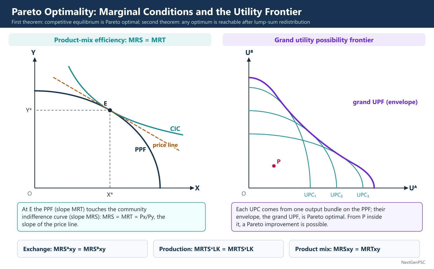
A state is Pareto optimal when no one can be made better off without making someone worse off (Pareto, 1906). It requires MRS equal across consumers, MRTS equal across goods and MRS = MRT. The first theorem says every competitive equilibrium is Pareto optimal; the second says any Pareto optimum can be reached by competition after lump-sum redistribution. Pareto optimality says nothing about distribution.
In simple words
Pareto optimality means resources are used so well that nobody can gain without someone else losing.
Think of sharing a pizza: if no slice is wasted and no swap would please both people, the sharing is Pareto optimal, even if one person got most of it.
Economists proved that perfect markets reach such efficient outcomes, but real markets fail through pollution, monopoly and missing information.
UPSC asks for the three marginal conditions, the two fundamental theorems and their limits.
1. Concepts and definitions
Welfare economics: the branch that judges economic states as better or worse for society; 'old' welfare economics (Pigou, The Economics of Welfare, 1920) used cardinal utility and interpersonal comparisons; 'new' welfare economics (from the late 1930s) uses ordinal utility and avoids such comparisons.
Pareto optimality: Vilfredo Pareto (Manuale di economia politica, 1906): a state is Pareto optimal (efficient) if no one can be made better off without making someone else worse off.
Pareto improvement: a change that makes at least one person better off and no one worse off.
Value judgements behind the criterion: individuals are the best judges of their own welfare; social welfare depends only on individual welfare; social welfare rises if one person is better off and none worse off.
2. The marginal conditions
Assumptions: two consumers, two goods, two factors, given tastes and technology, no externalities, convexity.
Exchange efficiency: the MRS between X and Y is equal for all consumers: MRSᴬxy = MRSᴮxy (on the consumption contract curve).
Production efficiency: the MRTS between L and K is equal in the production of every good: MRTSˣLK = MRTSʸLK (on the production contract curve, which maps into the production possibility frontier).
Product-mix (top-level) efficiency: every consumer's MRS equals the MRT, the slope of the PPF: MRSxy = MRTxy.
Second-order conditions: indifference curves and isoquants convex to the origin, and the PPF concave to the origin.
Utility possibility curve: each point on the consumption contract curve gives a pair (Uᴬ, Uᴮ); plotting them gives a utility possibility curve for one output bundle.
Grand utility possibility frontier: the envelope of the utility possibility curves from all points on the PPF where MRS = MRT; every point on it is Pareto optimal (Samuelson).
Infinity of optima: Pareto optimality gives a frontier, not a single best point; choosing among the points needs a social welfare function.
3. The fundamental theorems
First theorem: every competitive equilibrium is Pareto optimal, given complete markets, no externalities, no public goods and local non-satiation; it makes Adam Smith's invisible hand precise (Arrow, 1951; Debreu, 1959).
Why it holds: all consumers face the same price ratio, so MRSᴬ = MRSᴮ = Px/Py; all producers face the same factor prices, so MRTSˣ = MRTSʸ = w/r; profit maximisation gives MRT = MCx/MCy = Px/Py; hence MRS = MRT.
Second theorem: any Pareto optimal allocation can be reached as a competitive equilibrium after a suitable lump-sum redistribution of initial endowments, provided preferences and technologies are convex.
Meaning: efficiency and equity can be separated in principle: let markets allocate and use lump-sum transfers for distribution.
Market socialism link: Oskar Lange (1936–37) and Abba Lerner argued that a planner could mimic these conditions by setting prices equal to marginal cost.
4. Market failures and the second best
Externalities: Pigou (1920) showed that private and social marginal costs diverge; a Pigouvian tax equal to the marginal external cost restores efficiency; Ronald Coase (1960) argued that with clear property rights and low transaction costs, bargaining can do the same.
Public goods: non-rival and non-excludable goods are under-provided by markets; Samuelson's condition (1954) is ΣMRS = MRT.
Monopoly and increasing returns: P > MC violates the top-level condition.
Asymmetric information: George Akerlof's 'market for lemons' (1970); moral hazard and adverse selection in insurance and credit.
Theory of the second best: Richard Lipsey and Kelvin Lancaster (1956): if one Pareto condition cannot be met, it is generally not desirable to meet the remaining ones; piecemeal policy can lower welfare.
5. Diagrams to draw
Edgeworth box: the consumption contract curve joining the tangencies of A's and B's indifference curves; points off the curve allow Pareto improvements.
PPF and the top-level condition: a concave PPF in (X, Y) space with a community indifference curve tangent to it at E; the common slope gives MRS = MRT = Px/Py.
Utility possibility frontier: axes Uᴬ and Uᴮ; draw several utility possibility curves and their envelope, the grand UPF; add social indifference curves to locate the constrained bliss point.
6. Criticisms
Silent on distribution: an allocation in which one person has everything can be Pareto optimal; Sen observed that an economy can be Pareto optimal and still be 'perfectly disgusting'.
Status quo bias: the Pareto criterion cannot rank most real policies, because they always hurt someone.
Lump-sum transfers: rarely feasible; real taxes distort, so efficiency and equity cannot be fully separated.
Assumptions: perfect competition, complete markets, no externalities and convexity rarely hold together.
Individual sovereignty: preferences may be adaptive, misinformed or shaped by advertising.
7. Applications
India's subsidy reform: Direct Benefit Transfer (since 2013) moves subsidies closer to lump-sum income transfers and reduces price distortions.
Pigouvian instruments: the coal cess (introduced in 2010 as a clean energy cess) and the Carbon Credit Trading Scheme notified in 2023 address carbon externalities.
Public goods: defence, street lighting, disease surveillance and basic research are publicly funded because markets under-supply them.
Second best in India: the GST, with petroleum products and electricity outside its base and several rates, shows why partial reforms need second-best analysis.
8. Using it in the exam
10 marks: definition of Pareto optimality and the three marginal conditions.
15 marks: the first and second fundamental theorems with their logic and conditions.
20 marks: conditions, UPF diagram, theorems, market failures, second best and criticism with an Indian example.
Keywords: Pareto improvement, contract curve, MRS = MRT, utility possibility frontier, first and second theorems, lump-sum transfer, second best.
Definition: Pareto (1906): an allocation is Pareto optimal if no reallocation can make someone better off without making someone else worse off.
| Condition | Equation | Where shown | Achieved under competition because |
|---|---|---|---|
| Exchange efficiency | MRSᴬxy = MRSᴮxy | Consumption contract curve (Edgeworth box) | All consumers face the same Px/Py |
| Production efficiency | MRTSˣLK = MRTSʸLK | Production contract curve, PPF | All producers face the same w/r |
| Product-mix efficiency | MRSxy = MRTxy | Tangency of PPF and indifference curve | MRT = MCx/MCy = Px/Py = MRS |
Mains points
- Define Pareto optimality precisely and list the three marginal conditions with equations; add the second-order conditions for full marks.
- Show why competition satisfies each condition (common prices), which proves the first theorem in a few lines.
- Explain the second theorem and its policy meaning: separate efficiency from equity through lump-sum transfers, then note why such transfers are rarely possible.
- Draw the utility possibility frontier and show that Pareto optimality gives many optima; a social welfare function is needed to choose.
- Discuss market failures and the theory of second best (Lipsey and Lancaster, 1956) as limits.
- Use Indian examples: DBT as near-lump-sum transfer, carbon pricing, GST as a second-best reform.
Did you know?
- Pareto also gave the '80-20' observation: about 80% of Italy's land was owned by about 20% of the people, an idea now called the Pareto principle in management.
Compensation Criteria: Kaldor, Hicks, Scitovsky and Little
Compensation criteria rank changes that create gainers and losers. Kaldor (1939): gainers could compensate losers and still gain; Hicks (1939): losers could not bribe gainers to block the change. Scitovsky (1941) showed these tests can reverse and proposed a double criterion; Little added an explicit distributional judgement; Samuelson required the whole utility frontier to shift out.
In simple words
Most policies help some people and hurt others, like a new highway that helps travellers but takes farmers' land.
The compensation principle asks: could the winners pay the losers enough to make everyone at least as well off, and still have gains left over?
If yes, the change is called an improvement even if the payment is never made, which is why critics worry about fairness.
UPSC asks you to explain the Kaldor, Hicks, Scitovsky and Little criteria and their weaknesses.
1. The problem
Gainers and losers: most policy changes create both, so the Pareto criterion cannot rank them.
Robbins' challenge: Lionel Robbins (An Essay on the Nature and Significance of Economic Science, 1932) argued that interpersonal comparisons of utility are not scientific, which threatened welfare economics.
Response: compensation tests tried to rank changes without interpersonal comparisons, using money as the yardstick.
Compensation principle: a change is judged by whether the gainers could compensate the losers.
2. Kaldor criterion (1939)
Source: Nicholas Kaldor, 'Welfare Propositions of Economics and Interpersonal Comparisons of Utility', Economic Journal, 1939.
Statement: a change from A to B is an improvement if the gainers could compensate the losers and still be better off.
Hypothetical compensation: compensation need not actually be paid; whether it is paid is a separate, political question of distribution.
Kaldor's example: the repeal of the Corn Laws: landlords lost, but the gains of consumers and manufacturers exceeded the landlords' losses.
3. Hicks criterion (1939)
Source: J.R. Hicks, 'The Foundations of Welfare Economics', Economic Journal, 1939.
Statement: a change from A to B is an improvement if the losers could not profitably bribe the gainers to prevent it.
Relation: Hicks judges from the original position, Kaldor from the new one; together they form the Kaldor-Hicks criterion, the basis of cost-benefit analysis (total benefits exceed total costs, net present value above zero).
4. Scitovsky paradox and double criterion (1941)
Source: Tibor Scitovsky, 'A Note on Welfare Propositions in Economics', Review of Economic Studies, 1941.
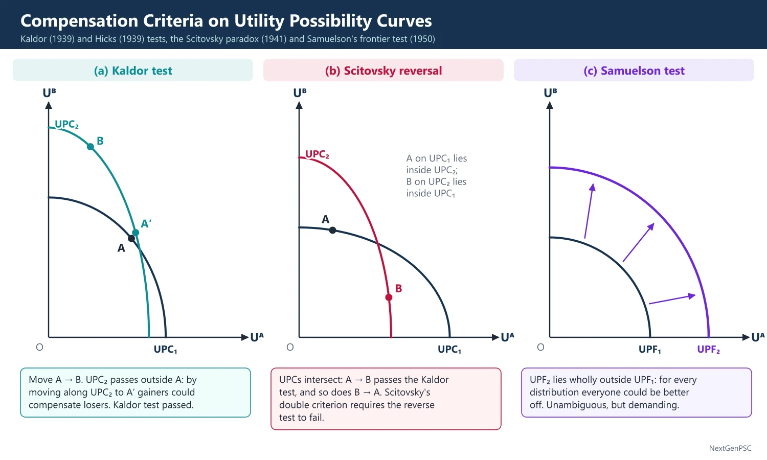
Paradox: when the utility possibility curves through A and B intersect, the Kaldor test can show that B is better than A and, after the move, that A is better than B; the criterion contradicts itself.
Cause: a change in output and distribution changes relative prices and hence the money valuations used in the test.
Double criterion: a move from A to B is an improvement only if (i) the gainers can compensate the losers (the Kaldor test passes for A to B) and (ii) the losers cannot bribe the gainers to reverse it (the Kaldor test fails for B to A).
Gorman (1955): showed that even the double criterion can give intransitive rankings across three or more states.
5. Little's criterion
Source: I.M.D. Little, A Critique of Welfare Economics (1950; second edition 1957).
Argument: compensation tests that ignore distribution are not value-free; distributional judgements must be made explicit.
Criterion: a change is an improvement if it passes the Kaldor-Hicks test, passes the Scitovsky reversal test, and the redistribution it causes is not judged to be bad; textbooks state the combination slightly differently, but all include an explicit distribution test.
Assessment: more realistic, but it brings back the value judgement that the new welfare economics tried to avoid.
6. Samuelson's utility possibility test (1950)
Statement: a change is an unambiguous improvement only if the new utility possibility frontier lies wholly outside the old one, so that for every distribution everyone could be better off.
Implication: tests based on a single point can mislead; comparisons need whole frontiers, which is very demanding.
7. Diagrams to draw
Kaldor test: axes Uᴬ and Uᴮ; draw UPC1 through A and UPC2 through B; if UPC2 passes outside (north-east of) A, the gainers could compensate the losers by moving along UPC2 to a point that dominates A.
Scitovsky reversal: draw UPC1 and UPC2 intersecting; place A on UPC1 inside UPC2 and B on UPC2 inside UPC1; the move A to B passes the Kaldor test and so does the move back from B to A.
Samuelson test: draw UPF2 lying entirely outside UPF1; only then is the change an unambiguous improvement.
8. Criticisms and debates
Potential versus actual: if compensation is not paid, the losers (often poorer) bear real losses; critics argue the Kaldor-Hicks test then carries a hidden value judgement in favour of the existing distribution of money.
Money metric: equal money values do not mean equal welfare when the marginal utility of income differs between rich and poor.
Inconsistency: reversals (Scitovsky) and intransitivity (Gorman).
Practical value: despite the flaws, the Kaldor-Hicks idea underlies the cost-benefit analysis of public projects.
9. Indian applications
Large dams: the Sardar Sarovar project brought large irrigation and drinking-water gains but displacement costs; rehabilitation and resettlement are attempts to pay actual compensation.
Land acquisition: the Right to Fair Compensation and Transparency in Land Acquisition, Rehabilitation and Resettlement Act, 2013 requires compensation of up to four times the market value in rural areas and two times in urban areas, plus rehabilitation, turning hypothetical compensation into actual payment.
Reform politics: tariff cuts or farm market reforms create diffuse gains and concentrated losses; the repeal in 2021 of the three farm laws of 2020 shows that losers who expect no compensation can block a potential Pareto improvement.
10. Using it in the exam
10 marks: the Kaldor and Hicks tests in one sentence each and the difference between them.
15 marks: the Scitovsky paradox with intersecting utility possibility curves and the double criterion.
20 marks: all criteria (Kaldor, Hicks, Scitovsky, Little, Samuelson), diagrams, criticisms and an Indian example such as land acquisition.
Keywords: potential compensation, Kaldor-Hicks, reversal paradox, double criterion, distributional value judgement, utility possibility frontier, cost-benefit analysis.
Definition: Kaldor (1939): a change is an improvement if the gainers could compensate the losers and still be better off.
| Criterion | Test | Main weakness |
|---|---|---|
| Pareto (1906) | Someone better off, no one worse off | Cannot rank changes with losers |
| Kaldor (1939) | Gainers could compensate losers and still gain | Compensation hypothetical; reversals possible |
| Hicks (1939) | Losers could not bribe gainers to block | Same as Kaldor; reversals possible |
| Scitovsky (1941) | Kaldor passes for A to B and fails for B to A | Intransitivity across three states (Gorman) |
| Little (1950) | Compensation tests plus redistribution not bad | Explicit value judgement needed |
| Samuelson (1950) | New utility frontier wholly outside old | Too demanding; rarely satisfied |
Mains points
- Begin with why compensation criteria arose: the Pareto criterion's silence on changes with losers and Robbins' attack on interpersonal comparisons.
- State Kaldor and Hicks precisely with their 1939 sources and stress that compensation is hypothetical.
- Draw intersecting utility possibility curves to show the Scitovsky reversal and explain the double criterion.
- Present Little's criterion as bringing distribution back explicitly, and Samuelson's frontier test as the strict version.
- Criticise: hypothetical compensation, money metric bias, intransitivity, and the hidden value judgement.
- Use India's land acquisition law (2013) or dam displacement as an example of turning potential compensation into actual compensation.
Did you know?
- Memory trick: 'Kaldor asks the Winners, Hicks asks the Losers': Kaldor tests whether winners can pay; Hicks tests whether losers can bribe.
Social Welfare Functions and Arrow's Impossibility Theorem
A social welfare function W = W(U₁, ..., Uₙ) (Bergson 1938, Samuelson 1947) ranks Pareto-optimal states and picks the constrained bliss point. Arrow (1951) proved that no rule can turn individual orderings into a rational social ordering while satisfying unrestricted domain, Pareto, independence of irrelevant alternatives and non-dictatorship. Ways out include single-peaked preferences and interpersonal comparisons.
In simple words
A social welfare function is a rule that tells society which outcome is best, combining everyone's well-being.
Imagine a family choosing a holiday spot by majority vote: sometimes the votes go round in circles, with hills beating the beach, the beach beating a city and the city beating hills.
Arrow proved that no voting rule can always avoid such problems while also being fair in four reasonable ways.
UPSC asks you to state Arrow's conditions, explain the theorem and discuss ways out.
1. The social welfare function
Purpose: Pareto optimality gives a frontier of efficient states; to choose among them, society needs a ranking based on value judgements about distribution.
Bergson-Samuelson SWF: Abram Bergson (Quarterly Journal of Economics, 1938) and Paul Samuelson (Foundations of Economic Analysis, 1947): W = W(U₁, U₂, ..., Uₙ), with ∂W/∂Uᵢ > 0, so the Pareto principle is built in.
Social indifference curves: combinations of individual utilities that give the same social welfare; they are convex to the origin if society values equality.
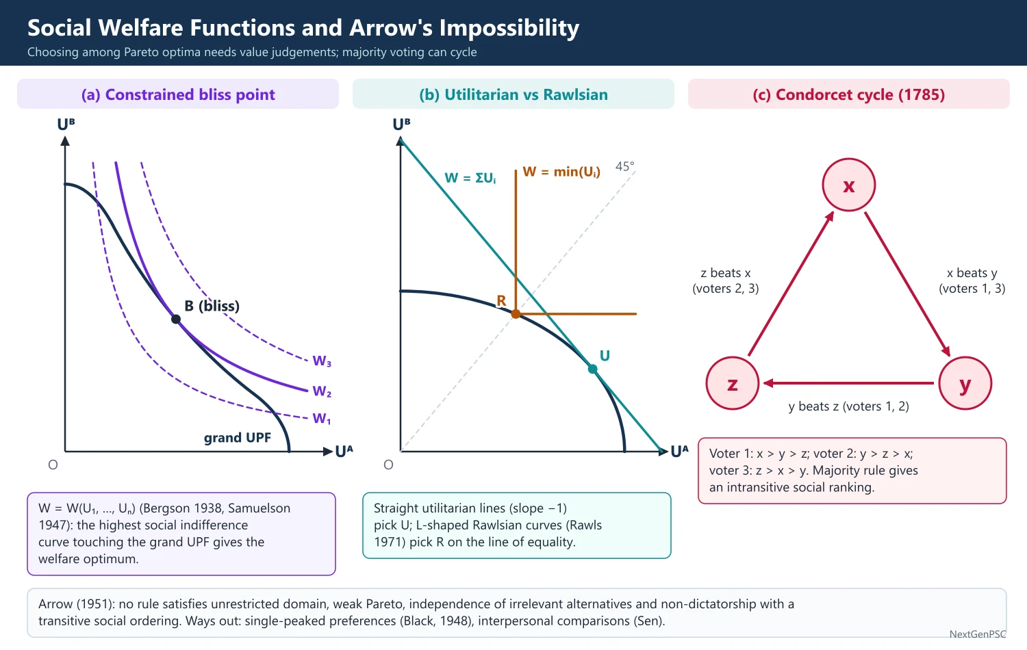
Constrained bliss point: the point where the highest attainable social indifference curve touches the grand utility possibility frontier; it is the welfare optimum.
Forms: utilitarian (Bentham) W = ΣUᵢ, with straight social indifference lines of slope −1; Rawlsian maximin (Rawls, A Theory of Justice, 1971) W = min(U₁, ..., Uₙ), with L-shaped curves; Bernoulli-Nash W = ΠUᵢ; the Atkinson (1970) family with an inequality-aversion parameter ε (ε = 0 utilitarian, ε → ∞ Rawlsian).
Where W comes from: the real question is how to build W from individual preferences by a democratic procedure; Arrow showed that this cannot be done under reasonable conditions.
2. The Condorcet paradox
Origin: the Marquis de Condorcet (1785) showed that majority voting can give cyclical social preferences.
Example: three voters and three options x, y, z; voter 1 ranks x over y over z; voter 2 ranks y over z over x; voter 3 ranks z over x over y.
Result: a majority prefers x to y, y to z and z to x, so the social ranking is intransitive and no option wins; the outcome depends on the order in which votes are taken (agenda power).
3. Arrow's impossibility theorem
Source: Kenneth Arrow, Social Choice and Individual Values (1951; second edition 1963).
Question: is there a rule (a social welfare function or 'constitution') that turns any set of individual preference orderings into a complete and transitive social ordering?
Condition U (unrestricted domain): the rule must work for every logically possible set of individual orderings.
Condition P (weak Pareto principle): if everyone prefers x to y, society must prefer x to y.
Condition I (independence of irrelevant alternatives): the social ranking of x and y depends only on individuals' rankings of x and y, not on their views about a third option z.
Condition D (non-dictatorship): there is no individual whose preference always becomes society's preference regardless of the others.
Collective rationality: the social ordering must be complete and transitive.
Theorem: with at least two individuals and at least three alternatives, no rule satisfies U, P, I and D together while giving a complete and transitive social ordering.
Intuition: the Pareto principle and independence together create 'decisive' groups; Arrow showed that a decisive group can be shrunk step by step to a single person, the dictator.
4. Ways out of the impossibility
Restrict the domain: Duncan Black (1948): if preferences are single-peaked along one dimension, majority voting is transitive and the median voter's preferred option wins.
Relax independence: positional rules such as Jean-Charles de Borda's count (1781) use intensity information and give complete rankings, but are open to manipulation.
Relax transitivity: Sen (1969) showed that requiring only quasi-transitivity allows a rule, but it creates an oligarchy with veto power (Gibbard).
Allow interpersonal comparisons: Sen showed that with comparable utilities (levels or units), utilitarian or Rawlsian SWFs become possible (Collective Choice and Social Welfare, 1970).
Gibbard-Satterthwaite theorem (1973, 1975): every non-dictatorial voting rule with three or more options can be manipulated by strategic voting.
5. Diagrams to draw
Constrained bliss: axes Uᴬ and Uᴮ; draw the grand utility possibility frontier concave to the origin and a family of convex social indifference curves; mark the tangency as the constrained bliss point B.
Forms of SWF: on the same axes draw straight utilitarian lines of slope −1 and L-shaped Rawlsian curves with corners on the 45° line; show that the Rawlsian optimum lies on or near the line of equality.
Condorcet cycle: draw a triangle x → y → z → x with arrows showing majority preference.
6. Debates
Samuelson's view: Arrow's theorem concerns a 'constitution' that aggregates many preference profiles, while the Bergson-Samuelson SWF is a single ordering for given tastes, so the SWF survives (debated).
Little (1952): questioned whether a social ordering must be as rational as an individual's.
Meaning for democracy: no voting system is perfect; each trades off some reasonable condition; this insight underlies modern social choice theory and mechanism design.
7. Applications
Voting systems in India: Lok Sabha elections use first-past-the-post; the President and members of the Rajya Sabha are elected by single transferable vote; each system meets some Arrow conditions and violates others.
Agenda-setting: committees and legislatures that vote on options in pairs can have outcomes fixed by the order of voting, as the Condorcet paradox predicts.
Coalition politics: multi-party bargaining over budgets or policies can produce shifting majorities, a practical face of cyclical preferences.
Policy SWFs: tax and transfer design implicitly uses an SWF; higher inequality aversion justifies more progressive taxes and targeted transfers.
8. Using it in the exam
10 marks: Arrow's four conditions plus collective rationality and the theorem in one line.
15 marks: the Condorcet paradox example, Arrow's theorem, and single-peakedness as a way out.
20 marks: the Bergson-Samuelson SWF with the bliss-point diagram, Arrow's theorem, ways out (Black, Sen) and the implications for democracy.
Keywords: social welfare function, social indifference curve, constrained bliss point, unrestricted domain, Pareto, independence of irrelevant alternatives, non-dictatorship, Condorcet cycle, single-peaked preferences.
Statement to quote: Arrow (1951): with at least three alternatives, no rule for aggregating individual orderings into a social ordering satisfies unrestricted domain, the Pareto principle, independence of irrelevant alternatives and non-dictatorship together.
| Condition | Meaning | If relaxed |
|---|---|---|
| Unrestricted domain (U) | Rule works for all preference profiles | Single-peaked preferences: majority rule works (Black, 1948) |
| Weak Pareto (P) | Unanimous preference respected | Rarely relaxed; imposed rules possible |
| Independence of irrelevant alternatives (I) | Ranking of x, y depends only on x, y | Borda count and other positional rules |
| Non-dictatorship (D) | No single decisive person | Dictatorship satisfies all others |
| Transitivity of social ordering | Complete and transitive ranking | Quasi-transitivity: oligarchy (Sen, 1969; Gibbard) |
Mains points
- Start from the need for an SWF: Pareto gives many optima, and an SWF picks the constrained bliss point; draw the diagram.
- Give the forms of SWF (utilitarian, Rawlsian, Bernoulli-Nash, Atkinson) and their social indifference curves.
- Explain the Condorcet paradox with a three-voter table before stating Arrow's theorem.
- State all of Arrow's conditions precisely (U, P, I, D and transitivity) with the number of voters and alternatives.
- Discuss ways out (Black's single-peakedness, Borda, Sen's interpersonal comparisons) and the Gibbard-Satterthwaite result.
- Conclude on implications for democracy and policy, with Indian voting systems as illustration.
Did you know?
- Memory trick for Arrow's conditions: 'U-P-I-D' (Unrestricted domain, Pareto, Independence, non-Dictatorship) plus transitivity.
Amartya Sen: Social Choice, Welfare and Capabilities
Amartya Sen (Nobel 1998) showed that Arrow's impossibility can be escaped by using more information, especially interpersonal comparisons. He proposed the welfare function W = μ(1 − G) and the Sen poverty index, proved the liberal paradox (1970), and built the capability approach: judge welfare by people's real freedoms to achieve valued functionings. His entitlement theory explains famines as a collapse of command over food.
In simple words
Amartya Sen asked what really makes a life go well: not just income or happiness, but what people are actually able to do and be.
Two people with the same income may live very differently if one is disabled or faces discrimination; a bicycle is useless to someone who cannot ride.
Sen calls these real freedoms capabilities, and his ideas shaped the Human Development Index and India's poverty debates.
UPSC asks about his response to Arrow, the liberal paradox, capabilities and famines.
1. Sen's place in welfare economics
Recognition: Amartya Sen (born 1933, Santiniketan) received the Nobel Memorial Prize in Economic Sciences in 1998 for his contributions to welfare economics, and the Bharat Ratna in 1999.
Core idea: Arrow's impossibility arises from using too little information; welfare judgements become possible once we allow interpersonal comparisons and look beyond utility to freedoms and capabilities.
Key works: Collective Choice and Social Welfare (1970); On Economic Inequality (1973); Poverty and Famines (1981); Commodities and Capabilities (1985); Development as Freedom (1999); The Idea of Justice (2009).
2. Informational broadening of social choice
Interpersonal comparability: with ordinal, non-comparable utilities Arrow's result holds; with comparability of levels the Rawlsian maximin becomes possible; with comparability of units the utilitarian sum becomes possible.
Weak Equity Axiom (On Economic Inequality, 1973): if person i has lower welfare than j at every income level, a just distribution should give i more income than utilitarianism would; it rejects pure utilitarianism, which ignores distribution.
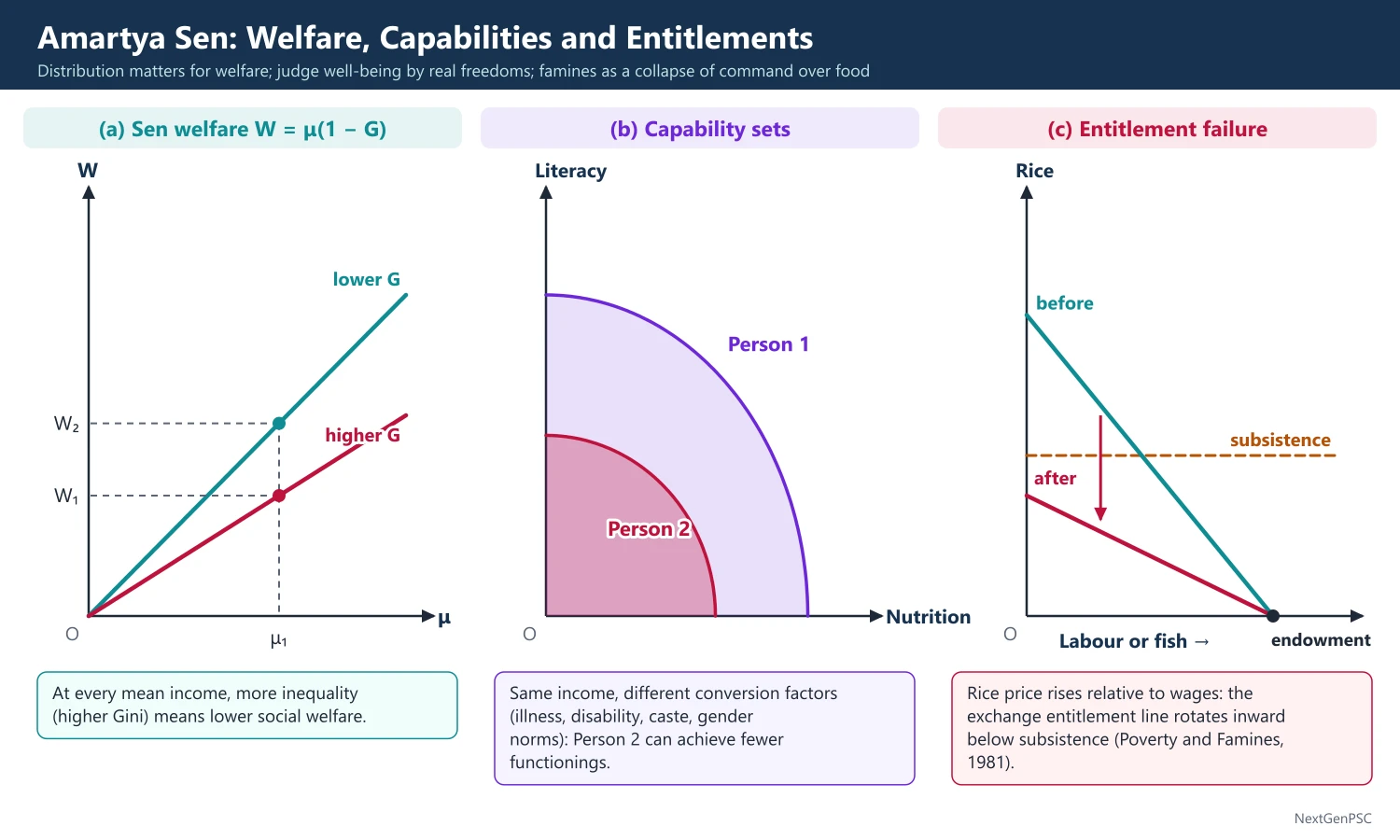
Sen's social welfare function: W = μ(1 − G), where μ is mean income and G the Gini coefficient; welfare rises with average income and falls with inequality (Sen, 1974).
Sen poverty index (Econometrica, 1976): P = H[I + (1 − I)Gₚ], where H is the headcount ratio, I the income-gap ratio and Gₚ the Gini coefficient among the poor; it satisfies the monotonicity and transfer axioms that the headcount ratio violates.
3. The liberal paradox
Source: 'The Impossibility of a Paretian Liberal', Journal of Political Economy, 1970.
Minimal liberalism: at least two persons are each decisive over at least one pair of alternatives that concern only their private lives.
Theorem: no social decision rule can satisfy unrestricted domain, the weak Pareto principle and minimal liberalism together.
Example: one copy of the book Lady Chatterley's Lover; a prude prefers that no one reads it, but if someone must, himself rather than the lewd; the lewd prefers that the prude read it rather than himself, and either rather than no one; liberal rights and the Pareto principle together produce a cycle.
Lesson: even the Pareto principle can conflict with individual liberty; welfarism (judging states only by utilities) is too narrow.
4. The capability approach
Functionings: the beings and doings a person values, such as being well nourished, healthy and literate, and taking part in community life.
Capabilities: the set of functionings a person can actually achieve, i.e. the real freedom to choose a life one has reason to value.
Conversion factors: the same income or primary goods give different capabilities depending on personal (disability, illness), social (gender norms, caste) and environmental factors.
Critique of utilitarianism: adaptive preferences (the deprived may learn to be content, so utility hides deprivation) and the neglect of rights and freedom.
Critique of Rawls: primary goods (income, rights, the bases of self-respect) are only means; people differ in turning them into freedoms.
Development as Freedom (1999): development is the expansion of real freedoms; Sen named five instrumental freedoms: political freedoms, economic facilities, social opportunities, transparency guarantees and protective security.
Nussbaum's extension: Martha Nussbaum proposed a list of ten central capabilities, whereas Sen deliberately leaves the list to public reasoning.
5. Entitlement approach to famines
Source: Poverty and Famines: An Essay on Entitlement and Deprivation (1981).
Entitlement: the set of commodity bundles a person can command through ownership and exchange (endowment, own production, trade, wages and transfers).
Argument: famines arise from the collapse of the entitlements of particular groups, not necessarily from a fall in total food availability (the 'FAD' view).
Bengal famine of 1943: Sen argued that food availability was not exceptionally low, while wartime inflation reduced the exchange entitlements of rural labourers, fishermen and artisans; some historians dispute parts of this reading.
Democracy and famine: Sen argued that no major famine has occurred in a functioning democracy with a free press, because governments face electoral and media pressure to act.
6. Influence on measurement
Human Development Index: launched by the UNDP in 1990 under Mahbub ul Haq, with Sen's capability approach as its foundation; it combines health, education and income.
Multidimensional Poverty Index: the Alkire-Foster method (2011) is used for the UNDP-OPHI global MPI (since 2010) and NITI Aayog's national MPI.
India's MPI: NITI Aayog's discussion paper (January 2024) estimated that multidimensional poverty fell from 29.17% in 2013–14 to 11.28% in 2022–23, with about 24.82 crore people moving out of it.
7. Diagrams to draw
Sen welfare: plot social welfare W on the vertical axis against mean income μ for two Gini values; the line with the higher G lies lower, showing that inequality reduces welfare at every mean income.
Capability set: draw the capability sets of two people with the same income in the space of two functionings (e.g. nutrition and literacy); the person with worse conversion factors (illness, discrimination) has a smaller set.
Entitlement collapse: draw a person's exchange entitlement line (labour or fish traded for rice); a rise in the rice price relative to wages rotates it inward, below the subsistence level.
8. Debates and applications
Criticism: capabilities are hard to measure and weigh; without a fixed list the approach can be vague; interpersonal comparisons remain value-laden.
The Idea of Justice (2009): Sen distinguished 'niti' (rules and institutions) from 'nyaya' (justice as actually realised) and argued for comparing feasible alternatives rather than identifying a perfectly just society.
India: Kerala's high life expectancy and literacy at modest income levels is the classic capability example; the National Food Security Act, 2013, the Right to Education Act, 2009 and rural employment guarantees are entitlement-protecting policies.
9. Using it in the exam
10 marks: functionings and capabilities, or the liberal paradox, in brief.
15 marks: Sen's response to Arrow through informational broadening and the SWF W = μ(1 − G).
20 marks: liberal paradox, informational broadening, capability approach, entitlement theory of famines and influence on HDI and MPI, with Indian examples.
Keywords: interpersonal comparability, weak equity axiom, liberal paradox, functionings, capabilities, conversion factors, entitlements, development as freedom.
Quotation (paraphrased): Sen sees development as a process of expanding the real freedoms that people enjoy.
| Contribution | Work and year | Key idea |
|---|---|---|
| Informational broadening of social choice | Collective Choice and Social Welfare (1970) | Interpersonal comparisons make SWFs possible |
| Liberal paradox | Journal of Political Economy (1970) | Pareto principle and minimal liberty conflict |
| Weak equity axiom; welfare W = μ(1 − G) | On Economic Inequality (1973); 1974 paper | Distribution matters for welfare |
| Sen poverty index | Econometrica (1976) | P = H[I + (1 − I)Gₚ] |
| Entitlement approach | Poverty and Famines (1981) | Famines from entitlement failure, not only food shortage |
| Capability approach | Commodities and Capabilities (1985); Development as Freedom (1999) | Welfare as real freedom to achieve functionings |
Mains points
- Present Sen as answering Arrow by enriching the information base: interpersonal comparability of levels or units makes Rawlsian or utilitarian SWFs possible.
- Explain the liberal paradox with the Lady Chatterley example and draw the lesson against pure welfarism.
- Define functionings, capabilities and conversion factors precisely, and contrast with utility and Rawls' primary goods.
- Give the formulas W = μ(1 − G) and P = H[I + (1 − I)Gₚ] for analytical depth.
- Use the entitlement approach for questions on famines and food security, citing the Bengal famine (1943) as Sen's case, noting the debate.
- Link to India: HDI, NITI Aayog's MPI (29.17% in 2013–14 to 11.28% in 2022–23), Kerala, NFSA 2013 and employment guarantees.
Did you know?
- Sen's first name was chosen by Rabindranath Tagore; 'Amartya' means 'immortal' or 'one who deserves to live beyond death'.
- Sen experienced the Bengal famine of 1943 as a nine-year-old in Santiniketan, which later shaped his work on entitlements.
Market Failure: Externalities, Public Goods and Asymmetric Information
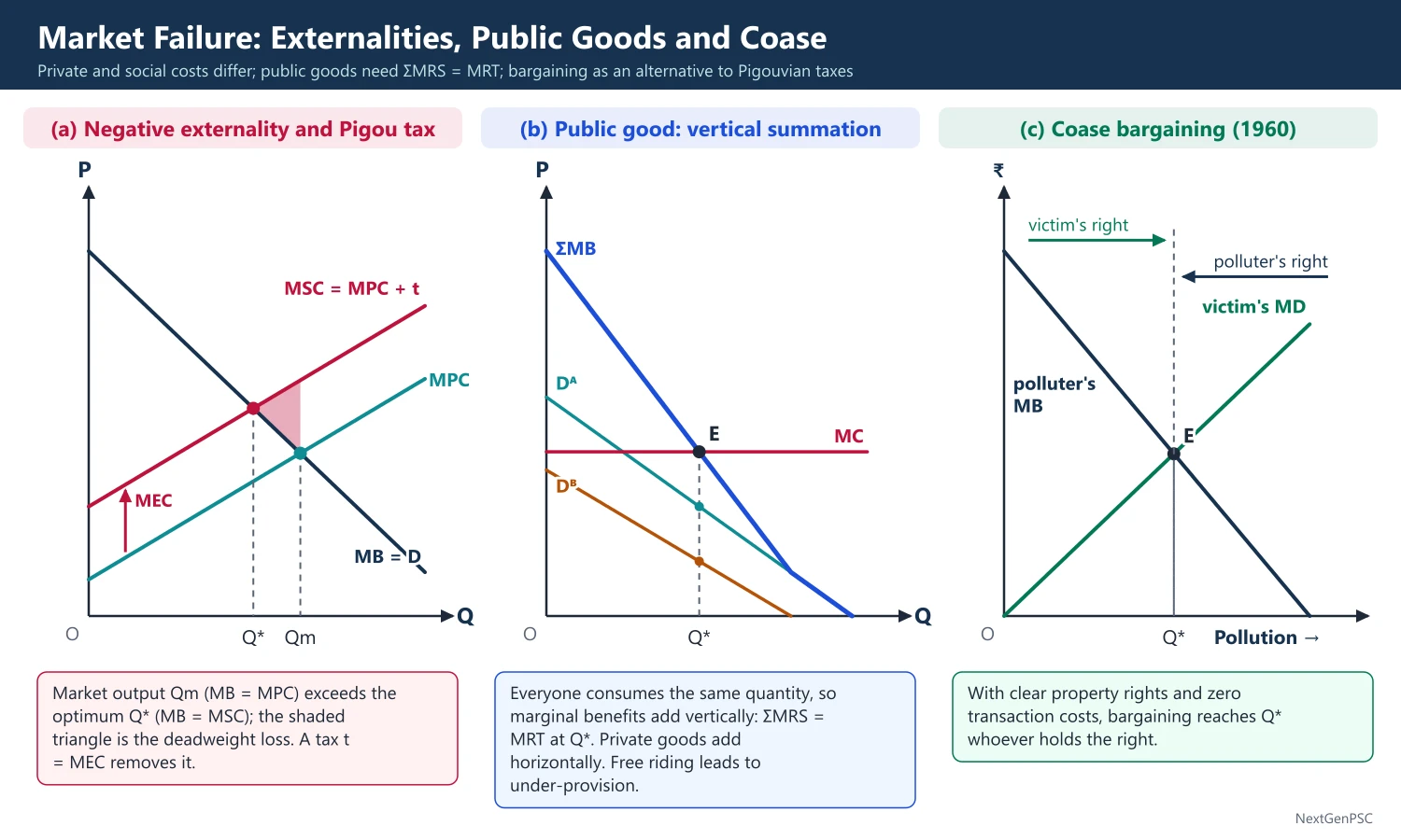
Market failure occurs when competitive markets do not reach a Pareto optimum. With externalities, private and social costs differ; Pigou proposed a tax equal to marginal external cost, while Coase (1960) showed that bargaining can solve the problem if property rights are clear and transaction costs are zero. Public goods need ΣMRS = MRT but suffer from free riding; asymmetric information causes adverse selection (Akerlof's lemons) and moral hazard, answered by signalling and screening.
In simple words
Market failure means a free market gives a wasteful result even when everyone acts sensibly.
A factory that pollutes a river does not pay for the harm to fishermen, so it produces too much; nobody pays for a streetlight because they can use it free; a used-car buyer cannot tell a good car from a bad one.
Governments and institutions fix these through taxes, rules, public provision and disclosure.
UPSC asks for the Pigouvian tax, the Coase theorem, the Samuelson condition and Akerlof's lemons.
1. What market failure means
Definition: the competitive outcome is not Pareto efficient because one or more conditions of the first fundamental theorem fail: externalities, public goods, asymmetric information, market power or incomplete markets.
Classification: Francis Bator's 'The Anatomy of Market Failure' (Quarterly Journal of Economics, 1958) classified failures by their source; this topic covers the three non-monopoly sources.
2. Externalities
Definition: an action of one agent directly affects the utility or production of others, not through prices; it can be negative (pollution, congestion) or positive (vaccination, research, beekeeping), and arise in production or consumption.
Pigou's analysis: A.C. Pigou (The Economics of Welfare, 1920) showed a divergence between marginal social net product and marginal private net product, building on Marshall's external economies.
Negative externality: MSC = MPC + MEC; the market produces where MPC = marginal benefit, which exceeds the social optimum where MSC = marginal benefit; the result is over-production and a deadweight loss.
Positive externality: MSB = MPB + MEB; the market under-produces.
Pigouvian tax and subsidy: a tax per unit equal to MEC at the optimal output makes the firm face social cost; a subsidy equal to the marginal external benefit corrects a positive externality.
Other instruments: standards (command and control), tradable permits (J.H. Dales, 1968), and Martin Weitzman's analysis (1974) of when to use prices (taxes) or quantities (permits) under uncertainty.
Double dividend: pollution tax revenue can replace distorting taxes, a debated claim of environmental tax reform.
3. The Coase theorem
Source: Ronald Coase, 'The Problem of Social Cost', Journal of Law and Economics, 1960.
Statement: if property rights are well defined and transaction costs are zero, private bargaining leads to the efficient outcome whoever holds the right; the assignment of rights affects only distribution.
Example: a factory and a fishery on a river; if the fishery holds the right, the factory pays it to allow pollution up to where the factory's marginal benefit equals the fishery's marginal damage; if the factory holds the right, the fishery pays it to cut pollution to the same level.
Reciprocal harm: Coase argued that harm is reciprocal: stopping the polluter harms the polluter, so the question is which harm is larger.
Limits: high transaction costs, many parties (free riding and hold-outs), asymmetric information, wealth effects and enforcement problems; the theorem is best read as showing why institutions and transaction costs matter (Coase received the Nobel Prize in 1991).
4. Public goods
Definition: Paul Samuelson ('The Pure Theory of Public Expenditure', Review of Economics and Statistics, 1954): goods that are non-rival (one person's use does not reduce another's) and non-excludable (people cannot be kept from using them).
Samuelson condition: efficiency requires ΣMRSᵢ = MRT, the sum of all consumers' marginal valuations equal to the marginal cost, because everyone consumes the same unit; for private goods each MRS = MRT.
Free-rider problem: each person gains from the good whether or not he pays, so people understate their preferences and voluntary provision falls short of the optimum.
Lindahl pricing (1919): each person pays a tax-price equal to his own marginal benefit; it is efficient but needs truthful revelation of preferences; Clarke (1971) and Groves (1973) designed demand-revealing mechanisms.
Impure goods: club goods are excludable but non-rival up to congestion (James Buchanan, 1965); common-pool resources are rival but non-excludable and suffer the 'tragedy of the commons' (Garrett Hardin, 1968), though Elinor Ostrom (Governing the Commons, 1990) showed communities often manage them well.
Merit goods: Richard Musgrave (1959): goods such as primary education and basic health that society wants provided irrespective of individual preferences.
5. Asymmetric information
Lemons model: George Akerlof, 'The Market for Lemons' (Quarterly Journal of Economics, 1970): buyers cannot tell good used cars from bad ones and offer the average value; owners of good cars withdraw; average quality and price fall, and the market can unravel.
Adverse selection: hidden characteristics before the contract: in insurance high-risk people buy more cover; in credit, Stiglitz and Weiss (1981) showed that higher interest rates attract riskier borrowers, so banks ration credit instead of raising rates.
Moral hazard: hidden action after the contract: insured people take less care; protected banks take more risk; it is a principal-agent problem.
Signalling: Michael Spence (1973): the informed party takes a costly action (such as acquiring education) that is cheaper for high-quality types, so a separating equilibrium can reveal quality; warranties are another signal.
Screening: Rothschild and Stiglitz (1976): the uninformed party offers a menu of contracts (e.g. insurance with different deductibles) so that types reveal themselves by their choice.
Remedies: disclosure rules, certification, warranties, deductibles and co-payments, collateral, credit bureaus and compulsory insurance; Akerlof, Spence and Stiglitz shared the Nobel Prize in 2001.
6. Diagrams to draw
Negative externality: axes Q and P; demand as marginal benefit; MPC rising and MSC above it by MEC; mark the market output Qm where MB = MPC and the optimum Q* where MB = MSC; shade the deadweight-loss triangle between Q* and Qm; show a Pigouvian tax shifting MPC up to pass through the optimum.
Public good: draw individual marginal benefit curves D_A and D_B and sum them vertically to get ΣMB; its intersection with MC gives the optimal quantity; contrast with horizontal summation for a private good.
Coase: horizontal axis pollution level; the polluter's marginal benefit falls and the victim's marginal damage rises; the efficient level is at their intersection, reached by bargaining from either end.
Lemons: show buyers' willingness to pay as the average quality of cars on sale, falling step by step as good cars leave the market.
7. Indian applications
Air pollution: stubble burning and urban smog are classic negative externalities; the National Clean Air Programme (2019) uses targets and standards, while Surat's emissions trading scheme for particulate matter (launched in 2019 by the Gujarat Pollution Control Board) uses tradable permits.
Market-based schemes: the Perform, Achieve and Trade scheme (from 2012) for industrial energy efficiency and the Carbon Credit Trading Scheme (2023).
Commons: free or flat-rate farm electricity has encouraged over-extraction of groundwater, a tragedy of the commons.
Asymmetric information: credit information companies, deposit insurance by the DICGC (cover raised to ₹5 lakh in 2020, with a moral hazard trade-off), RERA (2016) disclosure in real estate, and crop insurance under PMFBY (2016), which faces adverse selection and moral hazard.
Public goods: defence, disease surveillance and agricultural research are publicly funded because markets under-supply them.
8. Using it in the exam
10 marks: the Coase theorem with its conditions, or the Samuelson condition for public goods.
15 marks: the Pigouvian tax with a diagram, compared with the Coasian bargaining solution.
20 marks: market failure from externalities, public goods and asymmetric information, with remedies and Indian examples.
Keywords: MSC, MEC, Pigouvian tax, transaction costs, property rights, non-rival, non-excludable, free rider, ΣMRS = MRT, adverse selection, moral hazard, signalling, screening.
Definition: Coase (1960): with zero transaction costs and clear property rights, bargaining yields an efficient outcome whatever the initial allocation of rights.
| Source | Why the market fails | Key theorist | Remedies |
|---|---|---|---|
| Negative externality | MSC above MPC: over-production | Pigou (1920); Coase (1960) | Pigouvian tax, standards, tradable permits, bargaining |
| Positive externality | MSB above MPB: under-production | Pigou (1920) | Subsidy, public provision, patents |
| Public good | Non-rival, non-excludable: free riding | Samuelson (1954); Lindahl (1919) | Tax-financed public provision |
| Adverse selection | Hidden characteristics | Akerlof (1970) | Signalling, screening, mandatory insurance, certification |
| Moral hazard | Hidden action | Arrow; Stiglitz | Deductibles, co-payment, monitoring, collateral |
Mains points
- Draw the negative externality diagram with MPC, MSC and the deadweight-loss triangle, and show how a Pigouvian tax equal to MEC at the optimum corrects it.
- State the Coase theorem with both conditions (clear property rights, zero transaction costs) and explain why it often fails in practice.
- Derive the Samuelson condition ΣMRS = MRT and explain vertical summation and the free-rider problem.
- Distinguish adverse selection (hidden characteristics, before contract) from moral hazard (hidden action, after contract) with examples.
- Explain signalling (Spence) and screening (Rothschild-Stiglitz) as market responses to asymmetric information.
- Use Indian examples: stubble burning, Surat's emissions trading, groundwater commons, DICGC deposit insurance and crop insurance.
Did you know?
- Akerlof's 'lemons' paper was rejected by three journals, one reviewer saying it was too trivial, before the Quarterly Journal of Economics published it in 1970; it later earned him a share of the 2001 Nobel Prize.
UPSC Previous Year Questions: Welfare Economics
UPSC asked 19 question parts worth 265 marks on welfare economics between 2014 and 2026, all in Paper I. The most-asked topics are market failure (7 parts on public goods, externalities and asymmetric information), Pareto optimality (5 parts) and Arrow's theorem and social welfare functions (4 parts). Every question below has a model answer written to the UPSC word limit.
In simple words
Read the question, note the directive word (derive, distinguish, critically examine) and write your own answer first.
Then compare with the model answer: did you state the marginal conditions, name the economist and year, and draw the Edgeworth box or utility frontier?
Rewrite one weak answer each week until its structure matches the model.
1. Pareto Optimality and the Fundamental Theorems of Welfare Economics
Example 1 (UPSC 2026, 15 marks): Critically examine the statement, "Pareto optimality does not give a sufficient basis for ordering economic states from the perspective of social welfare". Can an economy with extreme inequality be considered Pareto efficient?
Paper and question: Paper I, Q2(b)
Approach: Define Pareto optimality, explain why it gives only an incomplete, distribution-blind ordering, and answer 'yes' to the second part with the contract-curve argument.
A state is Pareto optimal (Pareto, Manuale di economia politica, 1906) if no one can be made better off without making someone else worse off. The Pareto criterion ranks state A above B only if at least one person prefers A and no one prefers B.
Why it is not a sufficient basis: (i) it is incomplete: most policy changes create gainers and losers, and such states cannot be ranked; (ii) there are infinitely many Pareto optima, one for each initial distribution, and the criterion cannot choose among them; (iii) it is distribution-neutral, since it avoids interpersonal comparisons of utility; (iv) a Pareto-optimal state is not necessarily better than every non-optimal state.
Extreme inequality: yes, such an economy can be Pareto efficient. In an Edgeworth box, the corner allocation where one person owns everything lies on the contract curve: the poor person cannot be made better off without taking something from the rich. As Sen argued in Collective Choice and Social Welfare (1970), a state can be Pareto optimal with some people starving and others in luxury.
Diagram: the grand utility possibility frontier in (UA, UB) space; points near the axes (extreme inequality) and the middle point are all Pareto optimal; social indifference curves of a Bergson-Samuelson welfare function pick the bliss point on the frontier.
Hence the statement is correct: ranking states needs a social welfare function with explicit value judgements on distribution, which is why India pairs efficiency with redistributive policies such as food security and direct transfers.
Example 2 (UPSC 2024, 20 marks): Derive Pareto optimality conditions in production in a two commodities-two factors-two producers framework. Show that Pareto optimality does not necessarily guarantee for equity.
Paper and question: Paper I, Q2(a)
Approach: Set up the 2×2×2 production problem, derive MRTS equality by a Lagrangian or the Edgeworth production box, derive the production possibility curve, then show with the utility frontier that efficiency can coexist with inequity.
Framework: two goods X and Y, produced by two producers (one for each good) using two factors, labour L and capital K, in fixed total supply L̄ and K̄. Production functions X = X(Lₓ, Kₓ) and Y = Y(Lᵧ, Kᵧ) have diminishing MRTS.
Derivation: production is Pareto optimal when the output of one good cannot be raised without reducing the other. Maximise X(Lₓ, Kₓ) subject to Y(L̄ − Lₓ, K̄ − Kₓ) = Ȳ. The Lagrangian Z = X(Lₓ, Kₓ) + λ[Y(L̄ − Lₓ, K̄ − Kₓ) − Ȳ] gives ∂X/∂Lₓ = λ·∂Y/∂Lᵧ and ∂X/∂Kₓ = λ·∂Y/∂Kᵧ. Dividing, MPLₓ/MPKₓ = MPLᵧ/MPKᵧ, i.e. MRTSₓ = MRTSᵧ: the isoquants of the two producers must be tangent.
Edgeworth production box: the box has sides L̄ and K̄; X's isoquants are measured from the lower-left origin and Y's from the upper-right. Points of tangency form the production contract curve; off it, as at a point where isoquants cross, a reallocation of factors can raise both outputs.
Diagram: left panel, the production box with origins Oₓ and Oᵧ, tangency points E1, E2, E3 joined into the contract curve, and a non-tangency point A; right panel, the production possibility curve obtained by plotting the outputs at E1, E2, E3, concave to the origin, with A lying inside it.
Competitive attainment: with competitive factor markets each producer sets MRTS = w/r, and since both face the same w/r, MRTSₓ = MRTSᵧ holds automatically.
Not a guarantee of equity: every point on the contract curve, and hence the PPC, is Pareto optimal. Adding exchange efficiency (MRSᴬ = MRSᴮ) and MRS = MRT, every point on the grand utility possibility frontier is efficient, including points where one person gets almost everything. Which point is reached depends on the initial ownership of factors, not on efficiency.
Equity therefore requires a value judgement, a Bergson-Samuelson social welfare function, and lump-sum redistribution (the second fundamental theorem); in practice India relies on taxes and transfers.
Example 3 (UPSC 2022, 15 marks): A competitive equilibrium is both Pareto efficient and equitable. Do you agree? Justify your answer.
Paper and question: Paper I, Q2(c)
Approach: Agree with the first half (first fundamental theorem) and disagree with the second (equity depends on endowments); use the second theorem and the utility frontier.
Only half the statement is true. The first fundamental theorem of welfare economics (formalised by Arrow and Debreu in the 1950s) states that, with complete competitive markets, no externalities and locally non-satiated preferences, every competitive equilibrium is Pareto efficient.
Why efficient: all consumers face the same prices, so MRSᴬ = MRSᴮ = Px/Py (exchange efficiency); all producers face the same factor prices, so MRTSₓ = MRTSᵧ = w/r (production efficiency); and price equals marginal cost, so MRS = MRT (product-mix efficiency).
Why not equitable: the equilibrium reached depends on the initial endowments. If one person owns most land and capital, the competitive outcome is efficient but highly unequal. Efficiency is a property of the allocation, equity a value judgement on distribution, and the market makes no such judgement.
Second fundamental theorem: with convex preferences and technology, any Pareto-efficient allocation, including an equitable one, can be achieved as a competitive equilibrium after suitable lump-sum redistribution of endowments. Equity therefore needs state action; but lump-sum transfers are hard to design, and distortionary taxes create an efficiency-equity trade-off.
Diagram: Edgeworth box with two endowment points W1 and W2; competitive price lines through each reach different points on the contract curve, E1 (unequal) and E2 (more equal), both efficient.
Hence I disagree: competition delivers efficiency, while equity requires redistribution, as India attempts through progressive taxes and transfers such as PM-KISAN.
Example 4 (UPSC 2020, 15 marks): In an economy with only two commodities, two consumers and two producers with single factor of production, derive the necessary conditions for Pareto optimality in a 'perfect' economy.
Paper and question: Paper I, Q8(b)
Approach: Set up the economy (two goods produced with labour only, two consumers), derive the exchange, production and product-mix conditions by maximising one consumer's utility, and show how perfect competition satisfies them.
The economy: consumers A and B consume X and Y; producer 1 makes X = f(L₁), producer 2 makes Y = g(L₂), with L₁ + L₂ = L̄. Pareto optimality means maximising Uᴬ subject to Uᴮ = Ūᴮ, xᴬ + xᴮ = f(L₁) and yᴬ + yᴮ = g(L̄ − L₁).
Condition 1, exchange: the first-order conditions give MRSᴬₓᵧ = MRSᴮₓᵧ: both consumers' indifference curves are tangent (a point on the exchange contract curve).
Condition 2, production: with a single factor, production is efficient when no labour is idle and, if both producers could make the same good, the marginal product of labour in that good is equal across them; with each producer specialised, full employment of L̄ puts the economy on its production possibility curve.
Condition 3, product mix: shifting dL of labour from Y to X raises X by f′·dL and lowers Y by g′·dL, so MRTₓᵧ = g′(L₂)/f′(L₁) = MPLᵧ/MPLₓ. Optimality requires MRSᴬₓᵧ = MRSᴮₓᵧ = MRTₓᵧ.
Second-order conditions: convex indifference curves and a production possibility curve concave to the origin (diminishing marginal products).
Perfect economy: under perfect competition each consumer sets MRS = Px/Py; each producer hires labour until w = Px·f′ = Py·g′, so Px/Py = g′/f′ = MRT. Hence MRSᴬ = MRSᴮ = Px/Py = MRT, and the competitive equilibrium is Pareto optimal (first fundamental theorem), provided there are no externalities or public goods.
Diagram: the concave production possibility curve with an Edgeworth exchange box drawn inside it from the origin to the chosen output point; at the efficient point the slope of the indifference curves' common tangent equals the slope of the PPC.
Example 5 (UPSC 2019, 10 marks): What criteria will have to be satisfied to obtain a Pareto efficient allocation?
Paper and question: Paper I, Q5(c)
Approach: List the three marginal conditions (exchange, production, product mix) with the second-order and institutional conditions, briefly, with the Edgeworth box.
An allocation is Pareto efficient (Pareto, 1906) if no reallocation can make someone better off without making someone else worse off. In a 2 goods × 2 consumers × 2 factors economy it requires:
1. Efficiency in exchange: MRSᴬₓᵧ = MRSᴮₓᵧ; goods are distributed so that consumers' indifference curves are tangent (exchange contract curve).
2. Efficiency in production: MRTSˣₗₖ = MRTSʸₗₖ; factors are allocated so that the producers' isoquants are tangent (production contract curve), placing the economy on its production possibility curve.
3. Efficiency in product mix: MRSₓᵧ = MRTₓᵧ; the rate at which consumers are willing to substitute goods equals the rate at which the economy can transform one into the other.
Other criteria: second-order conditions (convex indifference curves and isoquants, a concave PPC) and the absence of externalities, public goods and monopoly; otherwise private marginal rates diverge from social ones.
Diagram: an Edgeworth box with consumers' indifference curves tangent along the contract curve; points off the curve allow a mutually beneficial trade.
Perfect competition satisfies all three because everyone faces the same prices.
2. Compensation Criteria: Kaldor, Hicks, Scitovsky and Little
Example 6 (UPSC 2025, 15 marks): What is Scitovsky Paradox? Explain it in the context of Kaldor-Hicks compensation test.
Paper and question: Paper I, Q2(c)
Approach: State the Kaldor-Hicks test, show with crossing utility possibility curves how it can approve a move from A to B and also the reverse move, and give Scitovsky's double criterion as the remedy.
Kaldor-Hicks test: Kaldor (1939) and Hicks (1939) held that a move from A to B is an improvement if the gainers could compensate the losers and still be better off, even if compensation is not paid.
Scitovsky paradox (Tibor Scitovsky, 'A Note on Welfare Propositions in Economics', Review of Economic Studies, 1941): the test can give contradictory verdicts. A move from A to B may pass the test, and the reverse move from B back to A may also pass it, so each state is judged better than the other.
Reason: a change in policy also changes the bundle of goods produced and its distribution, so each state has its own utility possibility curve (UPC). If the UPCs through A and B intersect, then from B redistribution along UPC_B can reach a point that dominates A, while from A redistribution along UPC_A can reach a point that dominates B.
Diagram: UA on the horizontal and UB on the vertical axis; two intersecting UPCs, UPC_A through A and UPC_B through B; B′ on UPC_B lies north-east of A, so B passes Kaldor-Hicks against A; A′ on UPC_A lies north-east of B, so A passes against B.
Scitovsky double criterion: B is better than A only if (i) the gainers could compensate the losers in moving to B (Kaldor-Hicks) and (ii) the losers could not bribe the gainers to oppose the move (the reversal test fails). This removes the contradiction.
Limits: even the double criterion ignores distribution and can be intransitive across three states (Gorman, 1955); Little (1950) added a distributional test.
Example 7 (UPSC 2015, 10 marks): How is Kaldor-Hicks compensation principle an improvement over Pareto optimality criterion? What are Scitovsky's views in this regard?
Paper and question: Paper I, Q2(c)
Approach: Explain the limitation of the Pareto criterion, how the Kaldor-Hicks potential compensation test overcomes it, and Scitovsky's paradox and double criterion.
The Pareto criterion can rank two states only if someone gains and nobody loses. Since almost every policy (a tariff cut, a dam, a road) hurts someone, it is silent on most real choices.
Improvement by Kaldor (1939) and Hicks (1939): a change is an improvement if the gainers could compensate the losers and still be better off, even without actual payment. This ranks changes with gainers and losers by asking whether total gains exceed total losses, the basis of cost-benefit analysis.
Scitovsky's views (1941): the Kaldor-Hicks test can be self-contradictory. If the utility possibility curves of the two states intersect, a move from A to B passes the test and so does the move back from B to A. Scitovsky therefore proposed a double criterion: B is better than A only if the move passes the Kaldor test and the reverse move fails it.
Diagram: two intersecting utility possibility curves in (UA, UB) space through A and B, each containing a point that dominates the other state.
Even the double test ignores whether compensation is actually paid, so distribution needs a separate judgement (Little, 1950).
3. Social Welfare Functions and Arrow's Impossibility Theorem
Example 8 (UPSC 2021, 20 marks): What is Buchanan's criticism of Arrow's theorem? Show how A. K. Sen proved Arrow's theorem without the overall consistency of social choice to avoid the criticism of Buchanan.
Paper and question: Paper I, Q8(c)
Approach: State Buchanan's 1954 objection that 'social rationality' (transitivity) is an illegitimate requirement, then explain Sen's demonstration that Arrow-type impossibility survives without any internal consistency of social choice, because the inter-profile conditions do the work; add the Paretian liberal result.
Arrow's theorem (Social Choice and Individual Values, 1951) shows that no rule aggregating individual orderings into a complete and transitive social ordering can satisfy unrestricted domain, weak Pareto, independence of irrelevant alternatives and non-dictatorship.
Buchanan's criticism ('Social Choice, Democracy, and Free Markets', Journal of Political Economy, 1954): requiring a transitive social ordering attributes individual rationality to 'society', an organic view of the state. Only individuals choose; collective decisions need not be consistent, and the intransitivity of majority voting can even be a virtue, since it prevents a permanent majority.
Sen's response: in 'Internal Consistency of Choice' (Econometrica, 1993) and 'Rationality and Social Choice' (American Economic Review, 1995), Sen reformulated the problem with social choice functions carrying no condition of internal consistency (no transitivity, no consistency across subsets) and still proved an Arrow-type impossibility.
How the proof works: the work is done by conditions linking choices across preference profiles: unrestricted domain, Pareto and independence of irrelevant alternatives. A group decisive over one pair is shown to be decisive over every pair (field expansion), and a decisive group can be shrunk to one person (group contraction), a dictator, without any step needing social transitivity.
Earlier result: Sen's 'Impossibility of a Paretian Liberal' (Journal of Political Economy, 1970) had already shown that even the minimal demand that social choice pick a best element (acyclicity, far weaker than transitivity) conflicts with the Pareto principle and minimal liberty, again sidestepping Buchanan's objection.
Implication: the impossibility arises from the poverty of information used (ordinal, non-comparable rankings), so Sen's constructive route is to admit interpersonal comparisons.
Example 9 (UPSC 2020, 10 marks): State Arrow's five reasonable conditions which a social welfare function must satisfy.
Paper and question: Paper I, Q5(a)
Approach: List Arrow's conditions precisely with a one-line meaning each, and state the theorem in one sentence.
Kenneth Arrow (Social Choice and Individual Values, 1951) asked whether individual preference orderings can be aggregated into a social ordering by a rule (a social welfare function) satisfying reasonable conditions:
1. Collective rationality: the social ordering must be complete and transitive (if society prefers x to y and y to z, it prefers x to z).
2. Unrestricted domain: the rule must work for every logically possible set of individual orderings.
3. Pareto principle (weak): if every individual prefers x to y, society must prefer x to y.
4. Independence of irrelevant alternatives: the social ranking of x and y depends only on individuals' rankings of x and y, not on their views of a third alternative z.
5. Non-dictatorship: there is no individual whose strict preference always becomes society's preference regardless of others.
Theorem: with at least three alternatives and two individuals, no social welfare function satisfies all five; majority voting can cycle (Condorcet's paradox).
Example 10 (UPSC 2017, 15 marks): "Pareto optimality conditions are necessary but not sufficient conditions for social welfare maximisation." Comment.
Paper and question: Paper I, Q2(a)
Approach: Explain why the marginal conditions define only the utility possibility frontier (necessary), and why a social welfare function is needed to choose the optimum on it (sufficient); draw the grand UPF with social indifference curves.
The Pareto conditions, MRSᴬ = MRSᴮ (exchange), MRTSˣ = MRTSʸ (production) and MRS = MRT (product mix), identify allocations at which no one can be made better off without making someone worse off.
Necessary: if any condition fails, a reallocation can raise someone's welfare without lowering anyone's, so social welfare cannot be at its maximum; any reasonable social welfare function that respects individual preferences (increasing in each person's utility) is maximised only on the Pareto frontier.
Not sufficient: the conditions are satisfied at infinitely many points, which together form the grand utility possibility frontier. They differ in distribution, and the Pareto criterion cannot rank one against another. A Pareto-optimal point with extreme inequality may even be judged worse than a non-optimal but more equal point.
Completing the analysis: Bergson (1938) and Samuelson (1947) introduced the social welfare function W = W(UA, UB), which embodies explicit value judgements about distribution. Its highest social indifference curve touches the grand UPF at one point, the 'constrained bliss' point, which is the welfare maximum.
Diagram: UA on the horizontal and UB on the vertical axis; the grand UPF concave to the origin; social indifference curves W1, W2, W3; W2 tangent to the UPF at B (bliss point); point C on the UPF lies on the lower W1, and point D inside the UPF lies on a higher curve than C, showing that a non-optimal point can be socially preferred to an optimal one.
Hence the statement is correct: efficiency must be combined with an equity judgement, which is why Arrow's search for a democratic social welfare function became important.
Example 11 (UPSC 2017, 15 marks): State and discuss Arrow Impossibility theorem. How does Sen modify it for social welfare maximisation?
Paper and question: Paper I, Q7(b)
Approach: State the theorem and its conditions, illustrate with the voting paradox, then explain Sen's modifications: interpersonal comparability (enabling Rawlsian and utilitarian SWFs), weaker rationality (quasi-transitivity) and the capability approach.
Theorem: Arrow (1951) proved that, with at least three alternatives, no social welfare function can turn individual orderings into a complete, transitive social ordering while satisfying unrestricted domain, the weak Pareto principle, independence of irrelevant alternatives and non-dictatorship.
Illustration: with three voters ranking (x, y, z), (y, z, x) and (z, x, y), majorities prefer x to y, y to z and z to x, a cycle (Condorcet's paradox). Any rule that avoids such cycles for every profile must violate one condition, ultimately giving one person decisive power.
Sen's modification 1, information: in Collective Choice and Social Welfare (1970) Sen traced the impossibility to Arrow's use of only ordinal, non-comparable utilities. If levels of welfare are comparable, the Rawlsian maximin is possible; if units are comparable, utilitarian summation is possible.
Modification 2, weaker rationality: Sen showed that if transitivity is relaxed to quasi-transitivity (only strict preference need be transitive), a non-dictatorial rule, the Pareto-extension rule, satisfies the other conditions; later work (Gibbard) showed this leads to oligarchy, so the gain is limited.
Modification 3, beyond utility: Sen argued welfare should be judged by capabilities, what people are able to do and be, rather than utility alone; this underlies the UNDP Human Development Index (1990), with Mahbub ul Haq.
Diagram: social indifference curves in (UA, UB) space: L-shaped curves for the Rawlsian maximin and straight lines of slope −1 for the utilitarian sum, each touching the utility possibility frontier at a different point.
Sen thus made social welfare judgements possible by admitting richer information.
4. Amartya Sen: Social Choice, Welfare and Capabilities
Example 12 (UPSC 2021, 10 marks): Using generalised Lorenz dominance show that lower inequality represents a higher social welfare state.
Paper and question: Paper I, Q1(b)
Approach: Define the Lorenz and generalised Lorenz curves, state Shorrocks' theorem linking GL dominance to welfare for all increasing, S-concave welfare functions, and show with a numerical example that lower inequality at the same mean gives higher welfare.
The Lorenz curve L(p) plots the cumulative share of income received by the poorest fraction p of the population. The generalised Lorenz curve (Shorrocks, 1983) scales it by mean income: GL(p) = μ·L(p), so it reflects both the size and the distribution of income.
Theorem: Atkinson (1970) showed that, for equal means, Lorenz dominance implies higher welfare under every additive welfare function with increasing, concave u. Shorrocks (1983) showed that x generalised-Lorenz-dominates y if and only if W(x) ≥ W(y) for all increasing, S-concave welfare functions, even with different means.
Example: mean income 50, x = (40, 60) and y = (20, 80): GL(0.5) is 20 for x and 10 for y, so x dominates. With u = √y, W(x) = 6.32 + 7.75 = 14.07 exceeds W(y) = 4.47 + 8.94 = 13.42: lower inequality gives higher welfare.
Diagram: p on the horizontal axis (0 to 1) and cumulative income per head on the vertical; the line of equality from the origin to μ; GL curve of x lying above that of y; both meeting at μ when p = 1.
The result connects inequality measurement with welfare and underlies Sen's welfare index W = μ(1 − G).
5. Market Failure: Externalities, Public Goods and Asymmetric Information
Example 13 (UPSC 2026, 10 marks): Differentiate between public goods and private goods. What is a 'Free Rider' problem?
Paper and question: Paper I, Q1(d)
Approach: Distinguish using rivalry and excludability (Samuelson, 1954), give examples, and define the free-rider problem with its consequence.
Following Samuelson ('The Pure Theory of Public Expenditure', 1954) and Musgrave, goods are classified by two properties.
Private goods are rival (one person's use reduces what is left for others) and excludable (non-payers can be kept out), e.g. food or a mobile phone; markets supply them efficiently, and market demand is the horizontal sum of individual demands.
Public goods are non-rival (an extra user costs nothing) and non-excludable, e.g. defence or street lighting; demand is the vertical sum of marginal valuations, and efficiency needs ΣMRS = MRT (the Samuelson condition).
Free-rider problem: since no one can be excluded, each person has an incentive to hide his true valuation and let others pay, hoping to enjoy the good free. If everyone does this, voluntary contributions fall short and the market under-provides or fails to provide the good.
Remedy: provision by the state financed through compulsory taxation, as with defence and public health programmes in India.
Example 14 (UPSC 2025, 10 marks): What are the major reasons for market failure? Explain the role of the government in this context.
Paper and question: Paper I, Q1(d)
Approach: List the main sources of market failure (public goods, externalities, asymmetric information, market power, incomplete markets) with one line each, then the corresponding government roles with Indian examples.
Market failure occurs when a free market fails to allocate resources efficiently, i.e. the outcome is not Pareto optimal (Francis Bator, 'The Anatomy of Market Failure', 1958).
Reasons: (i) public goods, non-rival and non-excludable, are under-provided because of free riding; (ii) externalities: when private and social costs or benefits differ, as with pollution or vaccination, output is too high or too low; (iii) asymmetric information causes adverse selection and moral hazard (Akerlof, 1970); (iv) market power (monopoly) restricts output and sets price above marginal cost; (v) incomplete markets, e.g. for long-term credit or insurance for small farmers.
Role of government: (i) direct provision of public goods financed by taxes; (ii) Pigouvian taxes, subsidies, standards or tradable permits for externalities, e.g. India's Carbon Credit Trading Scheme (2023); (iii) disclosure rules and regulators for information problems (SEBI, IRDAI); (iv) competition law (Competition Act, 2002) and regulation of natural monopolies; (v) institutions that fill missing markets, such as crop insurance.
Government action must weigh government failure (rent-seeking, poor information) against market failure.
Example 15 (UPSC 2024, 15 marks): Distinguish between public goods and private goods. Explain how market failure occurs in the case of public goods.
Paper and question: Paper I, Q4(b)
Approach: Distinguish public and private goods by rivalry and excludability, then show why the market fails for public goods: vertical summation and the Samuelson condition versus private provision with free riding, with a diagram.
Private goods are rival and excludable: a mango eaten by one cannot be eaten by another, and non-payers can be refused. Public goods (Samuelson, 1954) are non-rival (an extra user costs nothing) and non-excludable (non-payers cannot be shut out): defence, lighthouses, clean air.
Efficient provision: for private goods, market demand is the horizontal sum of individual demands, and efficiency requires each consumer's MRS to equal MRT. For a public good, each unit is consumed jointly, so its social value is the sum of all consumers' marginal valuations: efficiency requires ΣMRS = MRT (the Samuelson condition), i.e. the vertically summed demand curve must cut the marginal cost curve.
Why the market fails: (i) non-excludability creates the free-rider problem: each consumer understates his valuation, expecting others to pay; (ii) private suppliers cannot collect revenue from non-payers, so they supply little or nothing; (iii) even if exclusion were possible, charging a positive price for a non-rival good excludes users whose consumption costs nothing, a deadweight loss; (iv) the Lindahl solution (personalised tax prices equal to each person's marginal valuation) is efficient in theory but fails because people have no incentive to reveal true preferences.
Diagram: quantity of the public good on the horizontal axis and price on the vertical; individual demand curves DA and DB; their vertical sum ΣD; a horizontal MC line; the efficient output Q* where ΣD cuts MC; private provision Qₚ, smaller than Q*, where only one consumer's demand meets MC.
Public goods are therefore provided by the state through taxation, as in India's defence, policing and disease-surveillance programmes.
Example 16 (UPSC 2022, 15 marks): Give economic rationale for public expenditure on elementary education — a merit good.
Paper and question: Paper I, Q4(b)
Approach: Define a merit good (Musgrave), then give the economic rationale for public spending on elementary education: externalities, human capital and growth, information and credit failures, equity, with Indian policy (Article 21A, RTE 2009, Samagra Shiksha, PM POSHAN).
A merit good (Musgrave, The Theory of Public Finance, 1959) is one society judges people should consume more of than they would choose, because private choices under-value its benefits.
1. Positive externalities: an educated person benefits others through better citizenship, lower crime, better public health and the spread of ideas; since private demand reflects only private benefits, the market produces less than the social optimum (marginal social benefit exceeds marginal private benefit).
2. Human capital and growth: Schultz (1961) and Becker (1964) treated education as investment; endogenous growth models (Lucas, 1988) show that human capital raises the productivity of all factors, so public investment yields high social returns.
3. Information and myopia: poor parents may under-estimate the returns to schooling or face short horizons, preferring child labour income today.
4. Credit market failure: households cannot borrow against a child's future earnings, so poor families under-invest even when returns are high.
5. Equity and capabilities: education is a basic capability (Sen) and the main route to equality of opportunity; leaving it to the market would reproduce inequality across generations.
Indian policy: Article 21A (86th Amendment, 2002) and the RTE Act, 2009 guarantee free education at ages 6–14, supported by Samagra Shiksha (2018) and PM POSHAN.
Example 17 (UPSC 2018, 10 marks): How do externalities lead to market failure? How can this situation be remedied?
Paper and question: Paper I, Q5(d)
Approach: Define externalities, show with the MSC/MPC diagram how a negative externality causes over-production, and list remedies: Pigouvian tax, regulation, permits and Coasian bargaining.
An externality is a cost or benefit of an activity that falls on third parties and is not reflected in market prices (Pigou, The Economics of Welfare, 1920). Negative examples are factory pollution and stubble burning; positive ones are vaccination and research.
Market failure: a polluting firm produces where price equals its marginal private cost (MPC), ignoring the external cost; marginal social cost (MSC) = MPC + marginal external cost lies above MPC. The market output Qₘ exceeds the efficient output Q*, where demand meets MSC, causing a deadweight loss. With positive externalities, output is too low.
Diagram: quantity on the horizontal and price on the vertical axis; demand D; MPC and a higher MSC; market equilibrium at Qₘ (D = MPC) and the optimum at Q* (D = MSC); the triangle between MSC and D from Q* to Qₘ is the welfare loss; a tax equal to the marginal external cost at Q* shifts MPC up to pass through the optimum.
Remedies: (i) a Pigouvian tax equal to marginal external damage, or a subsidy for positive externalities; (ii) regulation and standards, e.g. Bharat Stage VI emission norms (2020); (iii) tradable permits that put a price on pollution; (iv) Coase (1960): if property rights are clear and bargaining costs low, private bargaining reaches the efficient outcome regardless of who holds the rights.
Example 18 (UPSC 2016, 15 marks): What is a Lemon Market? What is the role of signalling and screening in it? Explain.
Paper and question: Paper I, Q3(c)
Approach: Explain Akerlof's lemons model with the adverse-selection unravelling, then signalling (Spence) and screening (Stiglitz) as market responses, with examples.
A lemon market (George Akerlof, 'The Market for Lemons', Quarterly Journal of Economics, 1970) is one in which sellers know the quality of a product but buyers do not, as in used cars, where a bad car is a 'lemon'.
Mechanism: suppose good cars are worth ₹4 lakh and lemons ₹2 lakh to buyers, in equal numbers. Unable to tell them apart, buyers offer only the average, ₹3 lakh. Owners of good cars, who value them above ₹3 lakh, withdraw; the share of lemons rises, buyers lower their offer further, and in the limit only lemons are traded. This is adverse selection: bad quality drives out good, and mutually beneficial trades in good cars do not occur.
Signalling (Michael Spence, 1973): the informed side takes a costly action that low-quality types find too expensive to imitate, so it credibly reveals quality. Examples: warranties and certified pre-owned programmes for cars, educational degrees for workers (Spence's job-market model), brand reputation.
Screening (Joseph Stiglitz; Rothschild and Stiglitz, 1976): the uninformed side designs a menu of contracts that makes different types sort themselves. Examples: insurers offering low-premium/high-deductible and high-premium/low-deductible policies; banks using collateral requirements; employers using probation periods.
Diagram: a supply curve of used cars rising with price (average quality rises with price) and a demand curve that depends on expected quality; as price falls, average quality falls and demand shifts down, the market shrinking towards only lemons.
Akerlof, Spence and Stiglitz shared the 2001 Nobel prize; in India, certified used-car platforms and the Insurance Regulatory and Development Authority's disclosure norms are applications.
Example 19 (UPSC 2016, 20 marks): What is asymmetric information? How could it lead to adverse selection and market failure? Discuss.
Paper and question: Paper I, Q4(a)
Approach: Define asymmetric information, distinguish adverse selection (hidden type, before the contract) from moral hazard (hidden action, after), show with the lemons and insurance examples how markets fail, and discuss remedies.
Asymmetric information exists when one party to a transaction knows something relevant that the other does not: sellers know product quality, borrowers know their riskiness, the insured know their health. Standard welfare theorems assume full information, so asymmetry can make competitive outcomes inefficient.
Adverse selection (hidden characteristics, before the contract): the uninformed side cannot distinguish types and offers an average price, which attracts the worst types and drives away the best. In Akerlof's (1970) used-car market, good cars are withdrawn because buyers pay only for average quality; the market shrinks and may collapse to lemons only.
Insurance example: if an insurer charges a premium based on average risk, low-risk people find it too expensive and drop out, while high-risk people buy; average claims rise, the premium is raised, more low-risk people leave, and the market may unravel (a 'death spiral'). In credit markets, Stiglitz and Weiss (1981) showed that raising interest rates attracts riskier borrowers, so banks ration credit instead of raising rates.
Moral hazard (hidden action, after the contract): once insured or financed, people take less care because they do not bear the full cost, e.g. reckless driving after full insurance or risky lending by banks expecting a bail-out.
Diagram: insurance market with premium on the vertical and coverage on the horizontal axis; demand from high-risk buyers above that of low-risk buyers; an average-risk premium line above the low-risk willingness to pay, showing low-risk buyers dropping out.
Remedies: (i) signalling and screening (warranties, deductibles, collateral); (ii) mandatory pooling: compulsory or group insurance, as in Ayushman Bharat–PMJAY (2018) or employer health cover, which keeps low risks in the pool; (iii) disclosure regulation and credit bureaus (CIBIL) that reduce information gaps; (iv) co-payments and monitoring against moral hazard.
Asymmetric information is thus a major source of market failure, but appropriate institutions can restore much of the lost efficiency.
Mains points
- Pareto questions want the three marginal conditions (exchange, production, product-mix) with the Edgeworth box and the point that efficiency says nothing about equity.
- Compensation questions are answered with Kaldor (1939), Hicks (1939), the Scitovsky reversal (1941) on crossing utility possibility curves, and Little's distributional criterion.
- For Arrow, list the conditions precisely (unrestricted domain, weak Pareto, independence of irrelevant alternatives, non-dictatorship, transitive social ordering) and show Sen's ways out: interpersonal comparability and weaker consistency.
- Market failure answers score with a crisp classification (public goods, externalities, asymmetric information, market power) plus a remedy for each and an Indian example.
- Diagrams expected: Edgeworth box with contract curve, grand utility possibility frontier with social indifference curves, crossing UPFs for Scitovsky, and the marginal social cost diagram for externalities.
Did you know?
- Arrow proved his impossibility theorem in his 1951 doctoral thesis, published as Social Choice and Individual Values; Condorcet had already noticed the voting cycle at its heart in 1785.
Economics Optional: All chapters
- Exam Pattern, Syllabus and Strategy
- Price Determination and Theories of Distribution
- Market Structures
- Welfare Economics
- Theories of Employment, Income and Interest
- Money and Monetary Management
- Public Finance
- Theories of International Trade
- Trade Policy, Protection and the WTO
- Balance of Payments and Exchange Rates
- Theories of Growth
- Economic Development
- Indian Economy in the Pre-Independence Era
- Planning in India
- Agriculture before Liberalisation
- Industry before Liberalisation
- National Income, Poverty and Inequality
- Agriculture after Liberalisation
- Industry after Liberalisation
- External Sector after Liberalisation
- Public Finance and Fiscal Federalism in India
- Monetary System and the RBI
- Employment, Wages and Poverty Alleviation