
Economics Optional · UPSC Notes
Theories of Employment, Income and Interest — UPSC Economics Optional Notes
Free, exam-focused notes for UPSC Prelims and Mains, with Prelims tips and Mains points for every topic. 7 topics.
Open in the interactive reader: bookmarks, progress tracking and read-aloud.
Classical Theory of Employment and Output
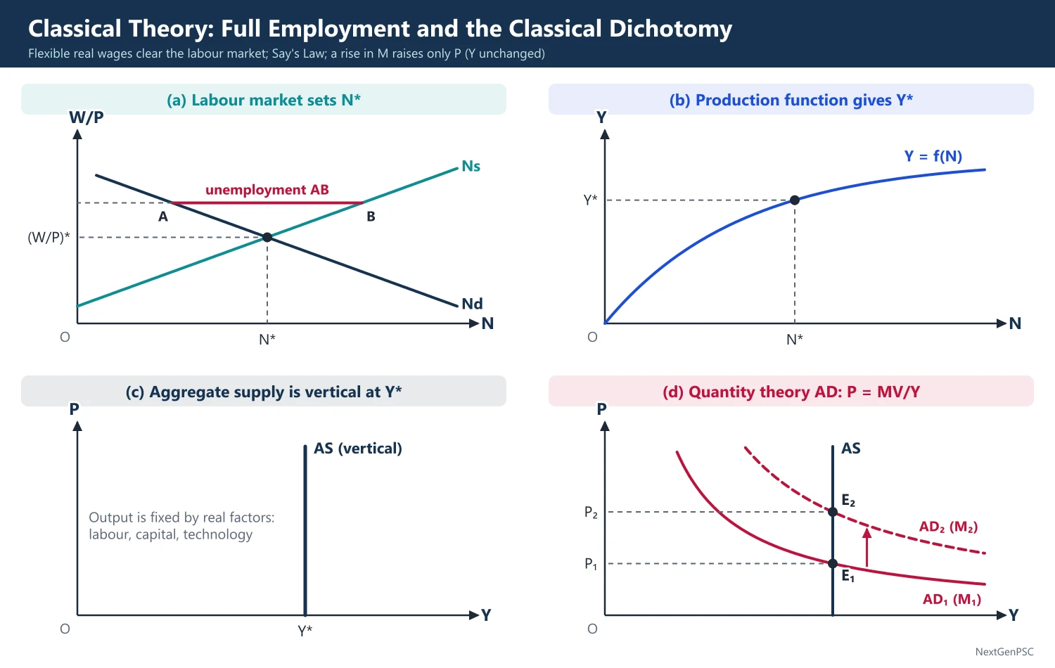
The classical theory holds that a market economy settles at full employment: flexible real wages clear the labour market, Say's Law ensures that output is demanded, the interest rate equates saving and investment, and money only fixes the price level (classical dichotomy). Output is set by real factors, so the aggregate supply curve is vertical. Keynes attacked it in 1936.
In simple words
The classical economists believed that anyone willing to work at the going wage would find a job, so mass unemployment could only be temporary.
If there were too many workers, wages would fall until employers hired them all, just as a vegetable seller cuts prices at the end of the day to sell everything.
Money, in their view, only changed prices, not real output; this is the classical dichotomy.
UPSC asks you to explain Say's Law, the classical model and Keynes' criticism.
1. The classical school
Who: Adam Smith, David Ricardo, J.B. Say and J.S. Mill; Keynes also counted Marshall and Pigou (Pigou's The Theory of Unemployment, 1933) as 'classical' because they shared the same conclusions.
Core beliefs: full employment is the normal state; output is determined by real factors (labour, capital, technology); money is neutral; wages, prices and the interest rate are flexible.
Method: long-run, equilibrium analysis in which markets clear through price adjustment.
2. Assumptions
Competition: perfect competition in goods and labour markets.
Flexibility: money wages and prices adjust freely; no money illusion, so labour supply and demand depend on the real wage W/P.
Say's Law: production creates income equal to its value, and that income is spent, either on consumption or (through saving) on investment.
Setting: closed economy, given capital stock and technology in the short run.
3. The model step by step
Production function: Y = f(N, K̄), with diminishing marginal product of labour.
Labour demand: profit-maximising firms hire until W/P = MPN, so labour demand Nd falls as the real wage rises.
Labour supply: Ns = g(W/P), rising with the real wage (workers trade leisure for income).
Labour market equilibrium: W/P adjusts so that Nd = Ns at full employment N*; output is Y* = f(N*), independent of the price level, so the aggregate supply curve is vertical.
Unemployment: only frictional or voluntary; any involuntary unemployment would be removed by money wage cuts (Pigou's prescription).
Say's Law: 'supply creates its own demand', Keynes' summary of J.B. Say (Traité d'économie politique, 1803); a general glut is impossible.
Saving and investment: the interest rate adjusts so that S(r) = I(r); saving rises and investment falls as r rises; thrift is spent on capital goods, so demand never falls short.
Price level: the quantity theory MV = PY with V constant and Y fixed at Y* makes P proportional to M (classical dichotomy and neutrality of money).
4. Comparative statics
Rise in money supply: P and W rise in the same proportion; real wage, N, Y and r are unchanged.
Rise in thriftiness: the saving curve shifts right; r falls; investment rises by the amount consumption falls; Y is unchanged.
Technical progress: MPN rises, labour demand shifts right; the real wage, employment and output rise.
Fiscal expansion: government borrowing raises r and crowds out an equal amount of private investment (full crowding out).
5. Diagrams to draw
Four-panel diagram: (a) labour market with Nd and Ns in (N, W/P) space meeting at N*; (b) production function Y = f(N) giving Y* at N*; (c) a vertical AS at Y* in (Y, P) space; (d) the quantity-theory AD curve P = MV/Y, a rectangular hyperbola; a rise in M shifts AD up and raises P with Y unchanged.
Saving-investment: axes S, I and r; a rising S(r) and falling I(r) meet at the equilibrium interest rate; a rise in thrift shifts S right and lowers r.
Wage cut: in the labour market show a real wage above W*/P with unemployment AB, and the fall in money wages that removes it.
6. Keynes' criticism
Say's Law fails in a monetary economy: income saved may be held as money (liquidity preference) instead of being invested, so aggregate demand can fall short of full-employment output.
Wage cuts: workers bargain over money wages, not real wages; a general cut in money wages lowers incomes and prices, so the real wage need not fall and employment need not rise.
Saving and investment: both depend mainly on income, not the interest rate; the interest rate is set by liquidity preference and the money supply.
Time horizon: 'In the long run we are all dead' (Keynes, A Tract on Monetary Reform, 1923).
Evidence: the Great Depression (1929–33), when US unemployment reached about a quarter of the labour force, contradicted the self-correcting view.
7. The classical reply and debates
Pigou (real balance) effect: Pigou (1943) argued that falling prices raise the real value of money holdings and hence consumption, so full employment can be restored in principle even in a liquidity trap.
Limits of the Pigou effect: falling prices raise the real burden of debt (Irving Fisher's debt deflation, 1933; Kalecki), and the effect may be small and slow.
Revival: monetarists and New Classical economists restored classical results for the long run through the natural rate of unemployment and rational expectations (later topics).
8. Relevance to India
Structural features: a large informal sector and disguised unemployment in agriculture mean the classical labour market, with a single flexible real wage, does not describe India well.
Measured unemployment: the Periodic Labour Force Survey 2023–24 put the unemployment rate at 3.2% (usual status, age 15 and above), but underemployment and low-productivity self-employment are large.
Supply-side policies: labour law consolidation into four codes (2019–20), ease of doing business and infrastructure reflect the classical stress on the supply side.
9. Using it in the exam
10 marks: Say's Law and its implication, or the classical dichotomy.
15 marks: the classical labour market and vertical AS with a diagram, plus Keynes' criticism.
20 marks: the full model (labour market, production function, saving-investment, quantity theory), comparative statics, the Pigou effect and Keynes' critique.
Keywords: Say's Law, flexible real wage, voluntary unemployment, loanable funds, neutrality of money, classical dichotomy, vertical AS, Pigou effect.
Quotation: 'Supply creates its own demand', Keynes' summary of Say's Law.
| Issue | Classical | Keynes (1936) |
|---|---|---|
| Normal state | Full employment | Underemployment equilibrium possible |
| Output determined by | Supply (real factors) | Effective demand |
| Wages | Flexible real wage clears labour market | Money wages rigid; cuts do not cure unemployment |
| Interest rate | Saving = investment (loanable funds) | Liquidity preference and money supply |
| Money | Neutral; affects only prices | Affects interest, investment and output |
| Policy | Laissez-faire | Active fiscal (and monetary) policy |
Mains points
- Present the classical model as a system: labour market, production function, saving-investment and quantity theory, with the four-panel diagram.
- State Say's Law precisely and explain how the interest rate makes it hold even with saving.
- Show the classical dichotomy: money changes P and W proportionally, leaving real variables unchanged.
- Give Keynes' criticisms point by point: money wage cuts, liquidity preference, saving and investment depending on income.
- Add the Pigou effect and its limits (debt deflation) for a balanced answer.
- Note the relevance and limits for India: informal labour, disguised unemployment, PLFS data.
Did you know?
- Say himself never wrote the exact words 'supply creates its own demand'; the phrase is Keynes' summary of Say's view.
Keynesian Theory of Income and Employment
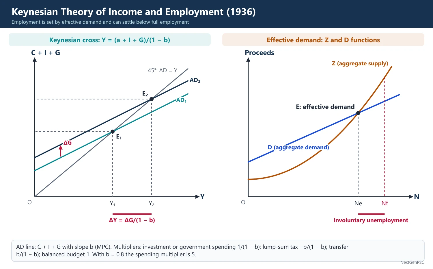
Keynes (General Theory, 1936) argued that employment is set by effective demand, the point where aggregate demand equals aggregate supply, and that this can occur below full employment (underemployment equilibrium). With C = a + bY, equilibrium income is Y = (a + I + G)/(1 − b) and the multiplier is 1/(1 − b). Deficient demand, not rigid real wages, causes involuntary unemployment, so government spending can raise output.
In simple words
Keynes said that jobs depend on how much people and the government want to spend; if spending is too low, factories cut output and workers lose jobs.
One person's spending is another's income: if the government builds a road, workers spend their wages at shops, shopkeepers spend again, and so on; this chain is the multiplier.
This explains why governments spend more during recessions.
UPSC asks you to explain effective demand, the multiplier and Keynes' break from classical theory.
1. Concepts and definitions
Source: J.M. Keynes, The General Theory of Employment, Interest and Money (1936), written during the Great Depression.
Aggregate supply price: the proceeds that entrepreneurs must expect in order to employ N workers; it rises with N (the Z function).
Aggregate demand price: the proceeds that entrepreneurs actually expect from the output of N workers (the D function).
Effective demand: the point where the aggregate demand function cuts the aggregate supply function; it fixes the level of employment, which need not be full employment.
Involuntary unemployment: workers willing to work at the current money wage (or even a little less) but unable to find jobs because demand is deficient.
2. Assumptions
Short run: capital stock, technology and labour force are given.
Prices: money wages are rigid downward, and prices are stable until full employment (in the simple model).
Closed economy: first without government; then government and foreign trade are added.
Demand-determined output: output adjusts to aggregate demand because there is spare capacity.
3. The consumption function
Psychological law: Keynes held that 'men are disposed, as a rule and on the average, to increase their consumption as their income increases, but not by as much as the increase in their income'.
Linear form: C = a + bY, where a is autonomous consumption and b the marginal propensity to consume (MPC), with b between 0 and 1.
Average propensity: APC = C/Y = a/Y + b falls as income rises; the saving function is S = −a + (1 − b)Y, with MPS = 1 − b.
Later theories: Simon Kuznets (1946) found the long-run APC roughly constant, which led to Duesenberry's relative income hypothesis (1949), Modigliani's life-cycle hypothesis (Modigliani and Brumberg, 1954) and Friedman's permanent income hypothesis (1957).
4. Equilibrium income and the multiplier
Two-sector equilibrium: Y = C + I with I autonomous; Y = a + bY + I gives Y = (a + I)/(1 − b); equivalently planned saving equals planned investment, S = I.
Investment multiplier: k = ΔY/ΔI = 1/(1 − b) = 1/MPS; with b = 0.8, k = 5; R.F. Kahn (1931) first gave the employment multiplier, and Keynes the investment multiplier.
Process: an extra ₹100 of investment raises income by 100, then by 80 as consumption, then 64, and so on: 100(1 + b + b² + ...) = 100/(1 − b).
Three-sector model: Y = C + I + G with C = a + b(Y − T); the government spending multiplier is 1/(1 − b), the lump-sum tax multiplier is −b/(1 − b), and the balanced budget multiplier is 1 (Haavelmo, 1945).
With proportional tax and imports: k = 1/[1 − b(1 − t) + m], where t is the tax rate and m the marginal propensity to import; leakages reduce the multiplier.
Paradox of thrift: if everyone tries to save more, income falls until saving returns to the level of investment; total saving does not rise (and falls if investment depends on income).
5. Diagrams to draw
Keynesian cross: axes Y (horizontal) and expenditure (vertical); draw the 45° line and the aggregate demand line C + I + G with slope b; equilibrium E where they cross; a rise in G shifts AD up by ΔG and income rises by ΔG/(1 − b).
Saving-investment: axes Y and S, I; an upward saving line −a + (1 − b)Y and a horizontal investment line; equilibrium where S = I; show the paradox of thrift by shifting S up and getting lower Y with the same S.
Effective demand: axes N and proceeds; draw the Z (aggregate supply) and D (aggregate demand) functions; their intersection gives employment Ne, short of full employment Nf.
6. Keynes versus the classics
Rejection of Say's Law: saving is a leakage that may not be matched by investment; output adjusts to demand.
Investment: depends on the marginal efficiency of capital and the interest rate, and is volatile because of 'animal spirits' (expectations).
Interest rate: a monetary phenomenon set by liquidity preference and money supply, not by saving and investment.
Policy: public works and deficit spending can raise demand when private demand is weak; monetary policy may fail in a liquidity trap.
7. Criticisms and debates
Neglect of supply: the simple model assumes spare capacity and fixed prices; at full employment extra demand raises prices.
Short-run focus: Keynes ignored capacity growth, later addressed by Harrod and Domar.
Relevance to developing countries: V.K.R.V. Rao (1952) argued that the multiplier works weakly in underdeveloped economies because supply is inelastic, a large part of income is spent on food, and disguised unemployment is structural, not demand-deficient.
Monetarist and New Classical critiques: crowding out, expectations and the Lucas critique (later topics).
8. Indian applications
Public capital expenditure: the Union Budget's capital expenditure was raised to ₹11.21 lakh crore in 2025–26 (budget estimate), justified by the higher multiplier of public capital spending.
COVID-19 response: the 2020 relief packages combined demand support (free foodgrains under PM Garib Kalyan Anna Yojana) with credit guarantees, a Keynesian response to a collapse of demand.
Rural demand: rural employment guarantee spending and income transfers such as PM-KISAN (2019) support consumption with a high MPC.
9. Using it in the exam
10 marks: the multiplier with derivation and a numerical example.
15 marks: effective demand and underemployment equilibrium with the Keynesian cross.
20 marks: consumption function, equilibrium, multipliers (investment, government, tax, balanced budget), paradox of thrift, criticism (including V.K.R.V. Rao) and Indian examples.
Keywords: effective demand, aggregate supply and demand functions, MPC, MPS, multiplier, leakages, balanced budget multiplier, paradox of thrift, involuntary unemployment.
Formula to quote: k = 1/(1 − MPC) = 1/MPS.
| Multiplier | Formula | Value when b = 0.8, t = 0, m = 0 |
|---|---|---|
| Investment / government spending | 1/(1 − b) | 5 |
| Lump-sum tax | −b/(1 − b) | −4 |
| Transfer payment | b/(1 − b) | 4 |
| Balanced budget | 1 | 1 |
| Open economy with proportional tax | 1/[1 − b(1 − t) + m] | 5 (falls as t and m rise) |
Mains points
- Define effective demand through the aggregate demand and supply functions, not just as 'total spending'.
- Derive the multiplier algebraically and through the geometric series, and give a numerical example.
- Show the Keynesian cross and the saving-investment diagrams with a shift and the new equilibrium.
- Contrast Keynes with the classics on Say's Law, wages, interest and policy in a short table.
- Cite V.K.R.V. Rao (1952) on the weak operation of the multiplier in underdeveloped economies; examiners value this Indian link.
- Use current Indian fiscal examples (capital expenditure push, COVID relief) carefully with years.
Did you know?
- Keynes joked that if the Treasury filled old bottles with banknotes, buried them in disused mines and let private firms dig them up, unemployment would fall; his point was that useful public works would be even better.
IS-LM Model and the Neo-classical Synthesis
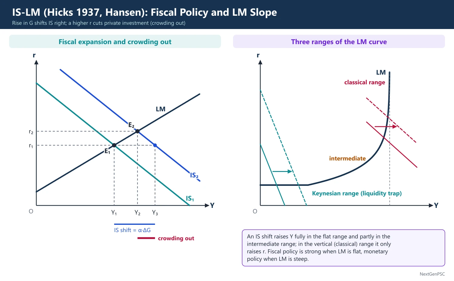
The IS-LM model (Hicks, 1937; Hansen) determines income and the interest rate together: the IS curve shows goods-market equilibrium and slopes down; the LM curve shows money-market equilibrium and slopes up. Policy effectiveness depends on the slopes: fiscal policy is strong when LM is flat (liquidity trap), monetary policy when LM is steep (classical case). The neo-classical synthesis treated Keynesian results as short-run outcomes of rigid wages and classical results as the long run.
In simple words
The IS-LM model links two markets: the market for goods (spending and income) and the market for money (interest rates).
Think of two roads crossing: one shows where spending balances income, the other where money demand balances money supply; the crossing gives the economy's income and interest rate.
It shows when government spending works better and when the central bank's interest rate changes work better.
UPSC asks you to derive both curves, show policy effects and explain the neo-classical synthesis.
1. Origin and concepts
Origin: J.R. Hicks, 'Mr. Keynes and the Classics: A Suggested Interpretation', Econometrica, 1937; developed by Alvin Hansen (A Guide to Keynes, 1953), hence the Hicks-Hansen model.
Purpose: Keynes' theory of income needs the interest rate (through investment), and his theory of interest needs income (through money demand); IS-LM solves both together, removing the indeterminacy of each theory alone.
IS curve: combinations of income Y and interest rate r at which the goods market is in equilibrium (investment = saving).
LM curve: combinations of Y and r at which the money market is in equilibrium (liquidity preference = money supply).
2. Deriving the IS curve
Equations: Y = C + I + G, with C = a + c(Y − T) and I = I₀ − br, where b measures the interest sensitivity of investment.
Solution: Y = α(A − br), where α = 1/(1 − c) is the multiplier and A = a − cT + I₀ + G is autonomous spending.
Slope: a lower r raises investment and, through the multiplier, income, so IS slopes down; it is flatter when b and α are large.
Shifts: a rise in G or I₀, or a tax cut, shifts IS to the right by α·ΔA.
3. Deriving the LM curve
Equations: real money demand L = kY − hr (transactions demand kY and speculative demand −hr); real money supply M/P is fixed by the central bank.
Solution: M/P = kY − hr gives r = (kY − M/P)/h.
Slope: higher income raises transactions demand; with fixed money supply, r must rise to cut speculative demand, so LM slopes up with slope k/h.
Shifts: a rise in M or a fall in P shifts LM to the right (down).
4. Equilibrium and policy multipliers
Equilibrium income: solving IS and LM gives Y = [h·α·A + α·b·(M/P)]/(h + k·α·b).
Fiscal multiplier: dY/dG = α·h/(h + k·α·b), smaller than the simple multiplier α because the rise in r crowds out investment.
Monetary multiplier: dY/d(M/P) = α·b/(h + k·α·b).
Liquidity trap (h very large): LM is horizontal; the fiscal multiplier approaches α and monetary policy has no effect (the extreme Keynesian case).
Classical case (h = 0): LM is vertical; fiscal policy has no effect on income (full crowding out) and monetary policy is fully effective.
Investment insensitive to r (b = 0): IS is vertical; monetary policy cannot change income, fiscal policy has its full multiplier.
Policy mix: fiscal expansion with monetary accommodation raises income without raising r; fiscal consolidation with monetary easing can keep output stable while lowering the deficit.
5. Diagrams to draw
Derivation of IS: four quadrants: investment schedule I(r); saving equals investment; saving function S(Y); and the resulting downward IS in (Y, r) space.
Derivation of LM: speculative demand L2(r), the money supply split between L1 and L2, transactions demand L1(Y), and the resulting upward LM.
Fiscal expansion: IS shifts from IS1 to IS2; equilibrium moves from E1 to E2 with higher Y and r; mark the horizontal shift of IS (α·ΔG) and the smaller actual rise in Y; the gap is crowding out.
Three ranges of LM: a horizontal Keynesian range at low r, an intermediate rising range and a vertical classical range; show that IS shifts raise Y only in the first two ranges.
6. The neo-classical synthesis
Meaning: a term popularised by Paul Samuelson (Economics, 1955 edition) for the view that Keynesian analysis applies in the short run when money wages and prices are rigid, while classical results hold in the long run when they are flexible.
Modigliani (1944): showed that in IS-LM, unemployment equilibrium depends on rigid money wages (except in the liquidity trap).
Pigou and Patinkin: the real balance effect shifts IS (or consumption) to the right as prices fall, so full employment is possible in theory even in a liquidity trap; Keynesian unemployment is then a matter of slow adjustment.
AD-AS and the Phillips curve: the synthesis added an aggregate supply side and the Phillips curve (Phillips, 1958; Samuelson and Solow, 1960) as a menu of inflation and unemployment for policy makers.
Policy era: the synthesis guided demand management in Western economies in the 1950s and 1960s until stagflation in the 1970s.
7. Criticisms and debates
Static and price-fixed: IS-LM ignores expectations, the dynamics of adjustment and the price level unless extended to AD-AS.
Hicks' own doubts: in 'IS-LM: An Explanation' (1980) Hicks admitted that combining a stock (money) equilibrium with a flow (saving-investment) equilibrium over a period is problematic.
Post-Keynesian critique: Joan Robinson and others called it 'bastard Keynesianism' for losing Keynes' emphasis on uncertainty (debated).
Modern versions: since central banks target interest rates, the LM curve is often replaced by a monetary policy rule (the IS-MP model of David Romer, 2000).
8. Indian applications
Monetary easing: the RBI cut the repo rate to 4% in May 2020 during the pandemic (a rightward LM shift) while the government expanded spending and guarantees (an IS shift).
Recent cycle: the repo rate was raised to 6.5% by February 2023 to fight inflation, then cut from 6.5% to 5.5% between February and June 2025 as inflation fell.
Crowding out debate: high central and state borrowing raises government bond yields, a crowding-out channel discussed in India's fiscal policy debates.
9. Using it in the exam
10 marks: derive the IS or LM curve with its slope and shift factors.
15 marks: relative effectiveness of fiscal and monetary policy with the three LM ranges.
20 marks: full IS-LM algebra, multipliers, crowding out, extreme cases, the neo-classical synthesis and its critics, with an Indian example.
Keywords: goods market, money market, interest sensitivity of investment, liquidity trap, classical range, crowding out, policy mix, real balance effect, neo-classical synthesis.
Quotable line: Hicks (1937) presented Keynes' theory and the classical theory as special cases of one general system.
| Case | Condition | Fiscal policy | Monetary policy |
|---|---|---|---|
| Liquidity trap (Keynesian) | LM horizontal (h very large) | Fully effective, no crowding out | Ineffective |
| Classical case | LM vertical (h = 0) | Ineffective, full crowding out | Fully effective |
| Interest-inelastic investment | IS vertical (b = 0) | Fully effective | Ineffective |
| Intermediate case | IS down, LM up | Partly effective, partial crowding out | Partly effective |
Mains points
- Derive IS and LM with equations and four-quadrant diagrams; state what determines each slope (α, b, k, h).
- Give the fiscal and monetary multipliers in IS-LM and show they are smaller than the simple multiplier.
- Explain the liquidity trap and the classical case as the two extremes, with a three-range LM diagram.
- Show crowding out as the gap between the horizontal IS shift and the actual rise in income.
- Present the neo-classical synthesis: Keynes in the short run with rigid wages, classics in the long run; mention Modigliani (1944), Pigou and Patinkin.
- Use Indian monetary-fiscal episodes (2020 easing, 2022–23 tightening, 2025 cuts) as illustrations.
Did you know?
- Hicks originally called the curves 'IS' and 'LL'; the label 'LM' (liquidity preference and money supply) became standard later through Hansen's work.
New Classical and New Keynesian Macroeconomics
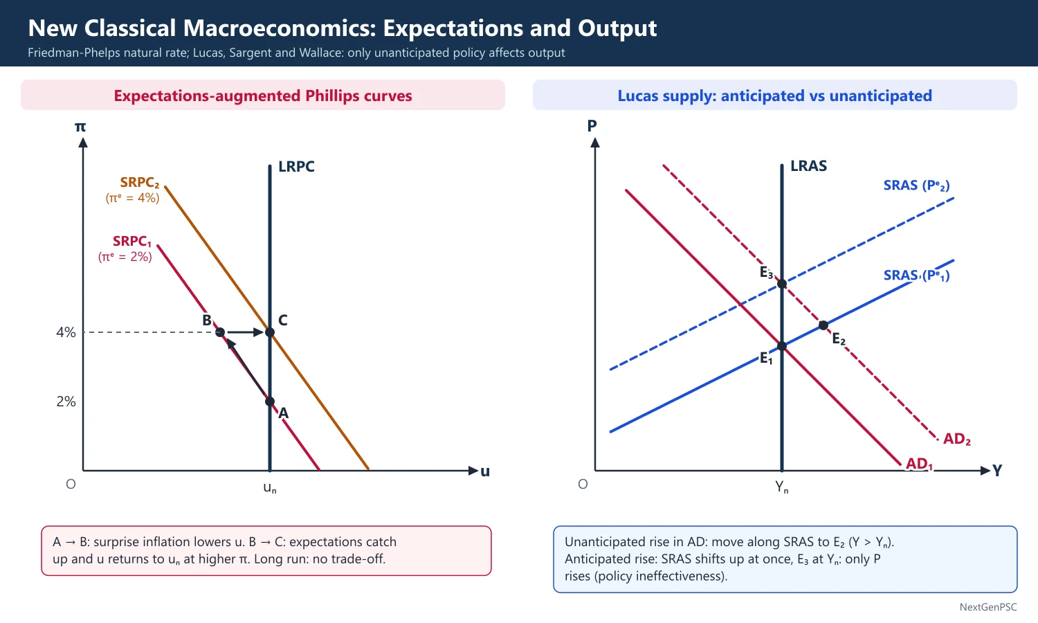
New Classical economists (Lucas, Sargent, Wallace, Barro) combined rational expectations with continuous market clearing: only unanticipated policy affects output (policy ineffectiveness), and the Lucas critique warns that policy changes alter behaviour. New Keynesians (Mankiw, Akerlof, Fischer, Taylor, Calvo) accept rational expectations but give micro-foundations for sticky prices and wages (menu costs, staggered contracts, efficiency wages), so demand policy still matters in the short run.
In simple words
These schools ask whether people can see government policy coming and adjust in advance.
New Classical economists say yes: if everyone expects the central bank to print money, shops raise prices at once and output does not change, like a magic trick that fails once the audience knows the secret.
New Keynesians reply that prices and wages are sticky because changing them is costly and contracts last a while, so policy can still help in the short run.
UPSC asks you to compare the two schools and explain rational expectations.
1. Background: monetarism and the natural rate
Original Phillips curve: A.W. Phillips (1958) found an inverse relation between wage inflation and unemployment in the UK; Samuelson and Solow (1960) presented it as a policy menu.
Natural rate hypothesis: Milton Friedman (AEA presidential address, 1968) and Edmund Phelps (1967–68) argued that there is a natural rate of unemployment uₙ set by real factors; policy can hold unemployment below it only by causing ever-rising inflation.
Expectations-augmented Phillips curve: π = πᵉ − β(u − uₙ); with adaptive expectations (πᵉ follows past inflation), the short-run curve shifts up whenever inflation exceeds expectations, and the long-run Phillips curve is vertical at uₙ.
Stagflation: the high inflation and high unemployment of the 1970s, after the oil shocks of 1973 and 1979, supported the natural-rate view.
2. New Classical assumptions
Rational expectations: John Muth (1961): agents use all available information, including knowledge of how policy works, so their forecasts are not systematically wrong.
Continuous market clearing: prices and wages adjust quickly so that markets clear.
Optimising agents: macro models are built on the choices of households and firms (micro-foundations).
Aggregate supply: output departs from its natural level only when the price level differs from what was expected.
3. New Classical model step by step
Lucas supply function: Y = Yₙ + α(P − Pᵉ), from Robert Lucas' 'islands' model (1972), in which producers confuse a general price rise with a rise in their relative price.
Policy ineffectiveness proposition: Thomas Sargent and Neil Wallace (1975): if the public anticipates a systematic monetary rule, Pᵉ moves with P and output stays at Yₙ; only unanticipated policy (surprises) moves output, and only temporarily.
Lucas critique (1976): the parameters of econometric models depend on the policy regime, so a model estimated under one policy cannot predict the effects of a new policy.
Ricardian equivalence: Robert Barro (1974): if households foresee that today's debt-financed tax cut means higher future taxes, they save the whole cut, and the fiscal stimulus has no effect (an idea discussed by Ricardo, who doubted it held in practice).
Time inconsistency: Finn Kydland and Edward Prescott (1977): a discretionary policy maker is tempted to create surprise inflation; the public anticipates this, so the result is higher inflation with no output gain; this supports rules and independent central banks.
Real business cycle theory: Kydland and Prescott (1982): fluctuations are efficient responses to real (technology) shocks, so stabilisation policy is unnecessary (see the investment and cycles topic).
4. New Keynesian economics
Aim: to explain, with rational, optimising agents, why prices and wages are sticky and why markets may not clear, so that demand shocks have real effects.
Menu costs: N. Gregory Mankiw (1985) and George Akerlof and Janet Yellen (1985): small costs of changing prices can cause large output fluctuations, because the private gain from adjusting price is second-order while the social cost of not adjusting is first-order.
Staggered contracts: Stanley Fischer (1977) and John Taylor (1979, 1980): wages are set for several periods and not all at once, so even fully anticipated monetary policy affects output in the short run.
Calvo pricing (1983): each firm can reset its price only with a fixed probability in each period, giving gradual price adjustment.
Efficiency wages: Shapiro and Stiglitz (1984): firms pay above market-clearing wages to reduce shirking and turnover, leaving involuntary unemployment.
Insider-outsider and hysteresis: Lindbeck and Snower: employed insiders keep wages high; Blanchard and Summers (1986): long recessions raise the natural rate itself (hysteresis).
New Keynesian Phillips curve: πₜ = β·Eₜπₜ₊₁ + κ·(yₜ − yₙ): current inflation depends on expected future inflation and the output gap.
5. The new neoclassical synthesis
Meaning: modern dynamic stochastic general equilibrium (DSGE) models combine New Classical tools (optimisation, rational expectations, real shocks) with New Keynesian price stickiness (Goodfriend and King, 1997).
Taylor rule (1993): i = r* + π + 0.5(π − π*) + 0.5(y − y*): the central bank raises the policy rate more than one-for-one with inflation; it describes how many central banks behave.
Policy lessons: credibility and anchored expectations matter; inflation targeting by independent central banks became standard from the 1990s.
6. Diagrams to draw
Expectations-augmented Phillips curves: axes u and π; draw short-run curves SRPC1 and SRPC2 for expected inflation of 2% and 4% and a vertical LRPC at uₙ; show a move from A to B (lower u, higher π) and back to C on LRPC as expectations adjust.
Lucas supply curve: axes Y and P; an upward short-run AS through (Yₙ, Pᵉ) and a vertical long-run AS at Yₙ; an anticipated rise in AD shifts AS up at once and leaves Y at Yₙ; an unanticipated rise moves along AS.
Menu costs: a monopolist's demand falls; show the small profit triangle gained by cutting price and the large welfare loss from not cutting.
7. Debates
Against New Classical theory: wages and prices are visibly sticky; rational expectations demand much information; recessions such as 2008–09 look like demand failures, not efficient responses.
Against New Keynesian theory: critics argue that menu costs are too small, and that DSGE models failed to anticipate the 2008 financial crisis because they had little role for finance.
Consensus: most economists accept rational (or at least forward-looking) expectations and a vertical long-run Phillips curve, along with short-run price stickiness that gives demand policy a stabilising role.
8. Indian applications
Inflation targeting: the amended RBI Act (2016) set up the Monetary Policy Committee and a CPI inflation target of 4% with a band of 2% to 6%, a framework built on anchoring expectations and rule-based credibility (time inconsistency).
Expectations data: the RBI's Inflation Expectations Survey of Households is used by the MPC as an indicator of how well expectations are anchored.
Sticky prices in India: administered prices (fuel, fertiliser, electricity tariffs) and annual wage revisions create stickiness that New Keynesian models capture.
9. Using it in the exam
10 marks: the policy ineffectiveness proposition, or the Lucas critique.
15 marks: the expectations-augmented Phillips curve and the natural rate with a diagram.
20 marks: compare New Classical and New Keynesian schools on assumptions, mechanisms and policy, with menu costs, staggered contracts and India's inflation targeting.
Keywords: natural rate, adaptive and rational expectations, Lucas supply function, policy ineffectiveness, Lucas critique, time inconsistency, menu costs, staggered contracts, efficiency wages, Taylor rule.
Quotable point: Sargent and Wallace (1975): systematic monetary policy cannot affect real output when expectations are rational and markets clear.
| Basis | New Classical | New Keynesian |
|---|---|---|
| Key names | Lucas, Sargent, Wallace, Barro, Kydland, Prescott | Mankiw, Akerlof, Yellen, Fischer, Taylor, Calvo, Stiglitz |
| Expectations | Rational | Rational |
| Markets | Clear continuously | Prices and wages sticky; may not clear |
| Anticipated monetary policy | No real effect | Real effect in the short run |
| Source of cycles | Price surprises, real (technology) shocks | Demand shocks with nominal rigidities |
| Policy view | Rules; no active stabilisation | Active, credible stabilisation (e.g. Taylor rule) |
Mains points
- Trace the sequence: Phillips curve, Friedman-Phelps natural rate, rational expectations, New Classical, New Keynesian.
- Write the expectations-augmented Phillips curve and the Lucas supply function, and draw the short- and long-run curves.
- State the policy ineffectiveness proposition and the Lucas critique with their authors and years.
- For New Keynesians, explain at least three sources of stickiness (menu costs, staggered contracts, efficiency wages) and Fischer's result that anticipated policy can matter.
- Mention time inconsistency as the basis for central bank independence and inflation targeting.
- Apply to India's flexible inflation targeting (2016) and the role of household inflation expectations.
Did you know?
- Lucas (1995), Kydland and Prescott (2004), Sargent (2011) and Phelps (2006) all received Nobel Prizes, showing how much the expectations revolution reshaped macroeconomics.
Theories of Interest Rate Determination and the Term Structure
The classical theory sets the interest rate where saving equals investment; the loanable funds theory (Wicksell, Robertson, Ohlin) adds bank credit and hoarding; Keynes' liquidity preference theory makes interest the reward for parting with liquidity, set by money demand and supply. Hansen showed each is indeterminate alone; IS-LM determines r and Y together. The term structure (yield curve) is explained by the expectations, liquidity premium, segmented markets and preferred habitat theories.
In simple words
The interest rate is the price of borrowing money, and economists disagree about what sets it.
Classical economists said it is like any price, set by how much people save and how much firms want to borrow; Keynes said it is the reward for giving up cash, like a fee for lending your umbrella on a rainy day.
The yield curve shows how interest rates differ for loans of different lengths, and it often signals where the economy is heading.
UPSC asks you to compare these theories and explain the term structure.
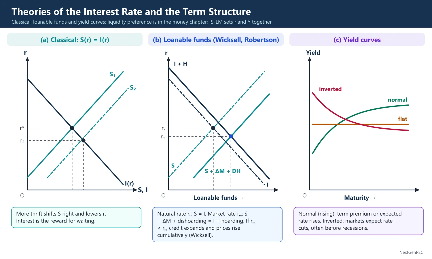
1. Concepts and definitions
Interest rate: the price paid for the use of loanable money over time, expressed as a percentage per year.
Nominal and real rates: Irving Fisher (The Theory of Interest, 1930): i = r + πᵉ, the nominal rate equals the real rate plus expected inflation (the Fisher equation).
Fisher's real theory: the real rate reflects time preference (impatience) and the investment opportunities available; Eugen von Böhm-Bawerk had earlier stressed the productivity of roundabout production and the discount on future goods.
2. Classical theory
Assumptions: full employment, given income, flexible interest rate, money neutral.
Supply of saving: S(r) rises with the interest rate, the reward for abstinence or waiting.
Demand for investment: I(r) falls with the interest rate, reflecting the diminishing marginal productivity of capital.
Equilibrium: r* where S(r) = I(r); a rise in thrift lowers r and raises investment; a rise in productivity raises r.
Criticism: it ignores the effect of income on saving, the role of money and hoarding, and assumes full employment.
3. Loanable funds (neo-classical) theory
Authors: Knut Wicksell (Interest and Prices, 1898), Dennis Robertson, Bertil Ohlin and Gunnar Myrdal.
Supply of loanable funds: saving + new bank credit (ΔM) + dishoarding + disinvestment.
Demand for loanable funds: investment + hoarding (adding to idle balances) + consumption loans.
Equilibrium: the interest rate equates the demand and supply of loanable funds; it recognises that money and credit affect the interest rate.
Wicksell's cumulative process: when the market (bank) rate is below the natural rate (the return on capital), investment exceeds saving, credit expands and prices rise cumulatively; when above, prices fall.
Strengths and criticism: it is realistic in including credit, but saving still depends on income, so the theory is indeterminate unless income is known (Hansen).
4. Keynes' liquidity preference theory
Definition: Keynes (General Theory, 1936): interest is the reward for parting with liquidity for a specified period, not a reward for saving.
Motives for holding money: transactions and precautionary motives, L1 = kY, depending on income; speculative motive, L2 = L2(r), falling as r rises because bond prices move inversely with r.
Speculative demand: each person holds a 'normal' rate in mind; if r is below it, people expect r to rise (bond prices to fall) and prefer money.
Equilibrium: the money supply M (fixed by the central bank) equals L1(Y) + L2(r); an increase in M lowers r, unless the economy is in a liquidity trap.
Liquidity trap: at a very low interest rate everyone expects r to rise, so speculative demand becomes perfectly elastic and extra money is simply held.
Criticism: it is also indeterminate without knowing income; it ignores real factors (productivity, thrift); it treats bonds and money as the only assets (Tobin's portfolio approach, 1958, broadened this).
5. The Hicks-Hansen synthesis
Indeterminacy: Alvin Hansen (Monetary Theory and Fiscal Policy, 1949) showed that the classical and loanable funds theories need income to locate the saving curve, and Keynes' theory needs income to locate L1, so none determines r alone.
Solution: the IS curve (from the classical and Keynesian goods market) and the LM curve (from liquidity preference) together determine both r and Y.
Stock versus flow: liquidity preference is a stock theory (demand for money holdings), loanable funds a flow theory (lending per period); in equilibrium they give the same result (debated by Hicks and others).
6. The term structure of interest rates
Yield curve: a plot of yields on bonds of the same risk against their maturity; it is normally upward sloping, may be flat, and is sometimes inverted.
Expectations hypothesis: Irving Fisher and Friedrich Lutz (1940): long-term rates equal the average of expected future short-term rates, e.g. i₂ = (i₁ + i₁ᵉ)/2 for a two-year bond; an upward curve signals expected rises in short rates.
Liquidity premium theory: J.R. Hicks (Value and Capital, 1939): lenders demand a premium for tying up funds longer, so long rates = average expected short rates + a term premium; this explains why the curve usually slopes up.
Segmented markets theory: J.M. Culbertson (1957): short and long bonds are not substitutes; each maturity's yield is set by its own demand and supply.
Preferred habitat theory: Franco Modigliani and Richard Sutch (1966): investors prefer certain maturities but will move to others for a sufficient premium, a blend of the above.
Inverted yield curve: when short rates exceed long rates, markets expect future rate cuts, often before recessions.
Risk structure: rates also differ by default risk, liquidity and tax treatment, giving spreads between government and corporate bonds.
7. Diagrams to draw
Classical: axes S, I and r; upward S(r) and downward I(r) meeting at r*; shift S right for more thrift.
Loanable funds: supply curve S + ΔM + dishoarding to the right of S; demand I + hoarding to the right of I; the market rate rₘ (where S + ΔM + dishoarding = I + hoarding) lies below the natural rate rₙ (where S = I).
Liquidity preference: axes money and r; a vertical money supply line M and a downward L curve flattening to horizontal at low r (liquidity trap); a rise in M from M1 to M2 lowers r except in the flat range.
Yield curves: axes maturity and yield; draw normal (rising), flat and inverted curves and label what each signals.
8. Indian applications
Deregulation: interest rates were largely administered before the 1990s; following the Narasimham Committee (1991), deposit and lending rates were freed in stages, ending with savings deposit rates in October 2011.
Lending benchmarks: the marginal cost of funds based lending rate (MCLR) from April 2016 and the external benchmark-linked lending rate (repo-linked) from October 2019 improved transmission of policy rates.
Small savings rates: after the Shyamala Gopinath Committee (2011), small savings rates were linked to government securities yields and are reset quarterly.
Government securities yield curve: the RBI watches the G-sec yield curve, with the 10-year bond as benchmark, for signals of inflation expectations and fiscal pressure.
9. Using it in the exam
10 marks: liquidity preference with the three motives and the liquidity trap, or the Fisher equation.
15 marks: loanable funds versus liquidity preference, with the indeterminacy critique.
20 marks: all theories, the Hicks-Hansen synthesis, the term structure theories with yield-curve diagrams and the Indian interest rate framework.
Keywords: time preference, productivity, loanable funds, natural and market rates, liquidity preference, speculative demand, liquidity trap, indeterminacy, yield curve, term premium, preferred habitat.
Definition to quote: Keynes (1936): interest is the reward for parting with liquidity for a specified period.
| Theory | Interest is set by | Nature | Main criticism |
|---|---|---|---|
| Classical (real) | Saving = investment | Real, flow | Ignores income and money; assumes full employment |
| Loanable funds (Wicksell, Robertson) | Demand = supply of loanable funds incl. credit and hoarding | Real and monetary, flow | Indeterminate without income |
| Liquidity preference (Keynes, 1936) | Money demand = money supply | Monetary, stock | Indeterminate without income; ignores real factors |
| Hicks-Hansen (IS-LM) | Goods and money markets together | General equilibrium | Static; fixed prices |
| Theory | Author and year | Key assumption | Explains |
|---|---|---|---|
| Expectations | Fisher; Lutz (1940) | Bonds of all maturities are perfect substitutes | Why yields move together; inverted curves |
| Liquidity premium | Hicks (1939) | Lenders need a premium for longer maturities | Why the curve usually slopes up |
| Segmented markets | Culbertson (1957) | Maturities are not substitutes | Independent movement of short and long rates |
| Preferred habitat | Modigliani and Sutch (1966) | Investors shift maturities for a premium | Both co-movement and upward slope |
Mains points
- Present the theories in sequence (classical, loanable funds, liquidity preference, IS-LM) and show how each improves on the last.
- Draw the liquidity preference diagram with the liquidity trap, and the loanable funds diagram with bank credit and hoarding.
- Explain Hansen's indeterminacy critique clearly; it is the bridge to IS-LM.
- Use the Fisher equation to distinguish nominal and real rates, especially for inflation questions.
- For the term structure, give all four theories with authors, a yield-curve diagram and what an inverted curve signals.
- Add India's interest rate deregulation, MCLR and external benchmark lending, and the G-sec yield curve.
Did you know?
- Memory trick for term structure theories: 'E-L-S-P': Expectations, Liquidity premium, Segmented markets, Preferred habitat.
Investment, Business Cycles and Aggregate Demand–Supply
Investment depends on the marginal efficiency of capital (the IRR of a project) compared with the interest rate, on the change in output (accelerator) and on Tobin's q. Samuelson (1939) showed that the interaction of the multiplier and accelerator can generate cycles; Hicks (1950) bounded them by a ceiling and a floor; real business cycle theory traces cycles to technology shocks. In the AD-AS model, AS is vertical with flexible wages (classical) and upward-sloping or flat with fixed money wages (Keynesian).
In simple words
Firms invest in machines and factories when the expected return beats the cost of borrowing, and when sales are rising fast.
Because investment reacts to changes in sales, a small rise in spending can set off a boom and a small fall a slump, like a swing that keeps moving once pushed.
The AD-AS model then shows whether extra demand raises output or only prices.
UPSC asks about MEC versus MEI, Tobin's q, the multiplier-accelerator model, Hicks' trade cycle and classical versus Keynesian AS.
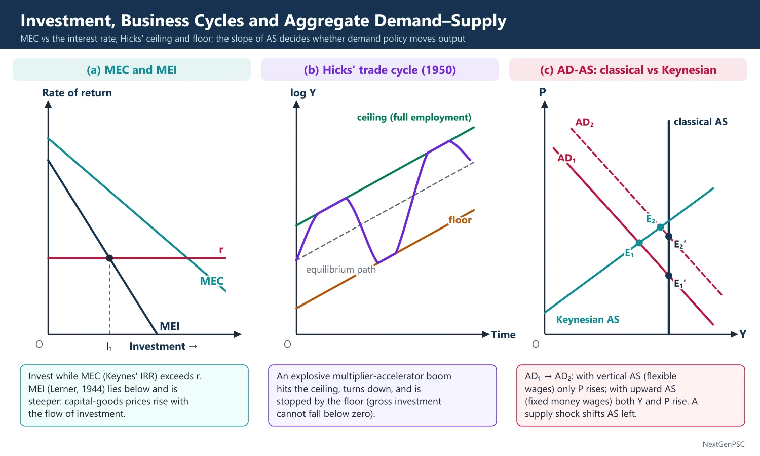
1. Theories of investment: MEC and MEI
Marginal efficiency of capital (MEC): Keynes (General Theory, 1936, chapter 11): the rate of discount that makes the present value of the expected returns from a capital asset equal to its supply price; invest while MEC exceeds the interest rate.
Equation: C = R₁/(1 + m) + R₂/(1 + m)² + ... + Rₙ/(1 + m)ⁿ, where C is the supply price, Rₜ the expected returns and m the MEC.
MEC schedule: slopes down because, as the capital stock grows, expected returns fall and the supply price of capital goods rises; it shifts with expectations ('animal spirits').
Marginal efficiency of investment (MEI): Abba Lerner (The Economics of Control, 1944): the rate of return when the supply price of capital goods rises with the rate of aggregate investment; the MEI curve lies below and is steeper than the MEC; MEC relates to the stock of capital, MEI to the flow of investment.
Net present value: NPV = −C + Σ Rₜ/(1 + i)ᵗ at the market interest rate i; invest if NPV is positive.
Internal rate of return: the discount rate that makes NPV zero; Keynes' MEC is the IRR; invest if IRR exceeds i; NPV is preferred when projects are mutually exclusive or cash flows change sign more than once.
2. The accelerator and Tobin's q
Simple accelerator: J.M. Clark (1917): with a fixed capital-output ratio v, desired capital K* = vY, so net investment Iₜ = v(Yₜ − Yₜ₋₁); investment depends on the change, not the level, of output.
Limits of the simple accelerator: it assumes no excess capacity and instant adjustment, and is asymmetric because gross investment cannot fall below zero.
Flexible accelerator: Goodwin (1951), Chenery (1952) and Koyck (1954): Iₜ = λ(K* − Kₜ₋₁), with 0 less than λ less than 1, so firms close only part of the gap each period.
Neo-classical theory: Dale Jorgenson (1963): desired capital depends on output and the user cost of capital (interest rate, depreciation, taxes, price of capital goods).
Tobin's q (1969): q = market value of a firm's capital / replacement cost of that capital; firms invest when q exceeds 1 because new capital is worth more than it costs.
Tobin's q in IS-LM: monetary easing lowers r and raises share prices, so q and investment rise; this adds a wealth and asset-price channel to the IS curve, making investment respond to stock markets as well as to r, so IS shifts with asset prices.
3. Business cycles: phases and causes
Phases: expansion (recovery and boom), peak, contraction (recession, and depression if severe) and trough.
Autonomous expenditure: changes in autonomous investment, government spending or exports start the process; the multiplier spreads the change to income, and the accelerator feeds it back to investment.
Other theories: Schumpeter's innovation waves, Keynes' collapse of the MEC, Kaldor's non-linear model (1940), monetary theories (Hawtrey, Friedman) and political business cycles.
4. Samuelson's multiplier-accelerator interaction (1939)
Source: Paul Samuelson, 'Interactions between the Multiplier Analysis and the Principle of Acceleration', Review of Economics and Statistics, 1939, building on Alvin Hansen.
Equations: Yₜ = G + Cₜ + Iₜ; Cₜ = b·Yₜ₋₁; Iₜ = v·(Cₜ − Cₜ₋₁); hence Yₜ = G + b(1 + v)·Yₜ₋₁ − b·v·Yₜ₋₂.
Outcomes: the path depends on b (MPC) and v (accelerator): if b(1 + v)² is less than 4v the path oscillates; with oscillation, cycles are damped if bv is less than 1, regular if bv = 1 and explosive if bv exceeds 1; without oscillation the path converges or explodes steadily.
Insight: a once-for-all rise in autonomous spending can generate cycles purely from the internal dynamics of the economy.
Criticism: realistic values of b and v tend to give explosive cycles, but actual cycles are neither explosive nor perfectly regular, which led to Hicks' constrained model.
5. Hicks' theory of the trade cycle (1950)
Source: J.R. Hicks, A Contribution to the Theory of the Trade Cycle (1950).
Assumptions: autonomous investment grows at a steady rate; the multiplier and accelerator values are such that the interaction is explosive; output grows along an equilibrium path.
Ceiling: the full-employment output line, growing at the natural rate; a boom hits the ceiling, output growth slows, and the accelerator turns investment down.
Floor: in the downswing, gross investment cannot fall below zero, so the accelerator stops working; autonomous investment and the multiplier set a floor from which recovery begins.
Result: cycles are bounded between the ceiling and the floor around a rising trend; criticism: the ceiling and floor are imposed rather than explained, and autonomous investment is assumed to grow steadily.
6. Real business cycle theory
Authors: Finn Kydland and Edward Prescott (1982); John Long and Charles Plosser (1983).
Mechanism: random technology (productivity) shocks, measured by the Solow residual, shift the production function; households choose to work and save more in good times (intertemporal substitution), so output, employment and investment move together.
Implications: cycles are efficient, money is neutral, and stabilisation policy is unnecessary or harmful.
Criticism: negative technology shocks large enough to cause recessions are hard to identify; labour supply is not that elastic; the theory struggles to explain the Great Depression and the 2008–09 recession, which look like demand collapses.
7. The AD-AS model
Aggregate demand: derived from IS-LM: a lower price level raises real money supply M/P, shifting LM right, lowering r and raising investment (Keynes effect), and raises real wealth and consumption (Pigou effect); so AD slopes down in (Y, P) space.
Classical AS: with flexible money wages and no money illusion, the labour market always clears at N*, so AS is vertical at Y*; demand changes affect only prices.
Keynesian AS with fixed money wages: with W fixed, a higher P lowers the real wage W/P, firms hire more and output rises, so AS slopes up; in the extreme Keynesian case with spare capacity AS is horizontal up to full employment (the reverse-L shape).
Short run and long run: money wages rise over time when unemployment is below the natural rate, shifting short-run AS up until the economy returns to the vertical long-run AS.
Shocks: a demand shock moves the economy along AS (output and prices move together); a supply shock such as the oil shocks of 1973 and 1979 shifts AS left (stagflation: higher prices, lower output).
8. Diagrams to draw
MEC and MEI: axes investment and rate of return; a downward MEC and a steeper MEI below it; the interest rate line gives the level of investment where it cuts MEI.
Hicks' trade cycle: axes time and log output; a rising ceiling line (full employment), a rising floor line below it and an equilibrium path between; draw output rising to the ceiling, moving along it, turning down to the floor, then recovering.
AD-AS: axes Y and P; a downward AD; a vertical classical AS at Y*; an upward Keynesian AS; show that an AD shift raises only P with vertical AS but raises both Y and P with upward AS; show a leftward AS shift for a supply shock.
Derivation of AD: upper panel IS-LM with LM shifting right as P falls; lower panel plotting the resulting (Y, P) pairs as AD.
9. Indian applications and the exam
India's cycles: monsoon shocks act as supply shocks to agriculture; real GDP contracted in 2020–21 because of the pandemic, the first annual fall since 1979–80; the investment cycle (gross fixed capital formation) has been led by public capital expenditure since 2021.
10 marks: MEC versus MEI, or Tobin's q.
15 marks: Samuelson's multiplier-accelerator model with conditions, or classical versus Keynesian AS.
20 marks: investment theories, multiplier-accelerator and Hicks' trade cycle with diagrams, real business cycle theory and AD-AS with an Indian example.
Keywords: MEC, MEI, NPV, IRR, accelerator, capital-output ratio, Tobin's q, ceiling and floor, real business cycle, Solow residual, Keynes effect, Pigou effect, vertical AS.
Definition to quote: Keynes (1936): the MEC is the rate of discount that equates the present value of the expected returns of a capital asset with its supply price.
| Condition on b and v | Path of income |
|---|---|
| b(1 + v)² less than 4v and bv less than 1 | Damped oscillations (converge to equilibrium) |
| b(1 + v)² less than 4v and bv = 1 | Regular oscillations of constant amplitude |
| b(1 + v)² less than 4v and bv greater than 1 | Explosive oscillations |
| b(1 + v)² ≥ 4v and bv less than 1 | Monotonic convergence |
| b(1 + v)² ≥ 4v and bv greater than 1 | Monotonic explosion |
| Basis | Classical AS | Keynesian AS |
|---|---|---|
| Money wages | Flexible | Fixed (rigid downward) |
| Shape | Vertical at full employment Y* | Upward-sloping, or horizontal up to full employment |
| Effect of AD increase | Only prices rise | Output and prices rise |
| Policy implication | Demand policy ineffective | Demand policy can raise output |
Mains points
- Define MEC with its equation and distinguish it from MEI (stock versus flow, Lerner, 1944); link MEC to IRR and contrast with NPV.
- Explain the simple and flexible accelerator and Tobin's q, and show how q adds an asset-price channel to IS-LM.
- Write Samuelson's second-order difference equation and give the conditions for damped, regular and explosive cycles.
- Draw Hicks' ceiling-floor diagram and explain why the accelerator stops working in the downswing.
- Contrast Keynesian (demand-driven) and real business cycle (technology-driven) explanations of cycles.
- Derive AD from IS-LM and compare classical (vertical) and Keynesian (fixed money wage) AS, with demand and supply shocks.
Did you know?
- Samuelson wrote his multiplier-accelerator paper as a 24-year-old graduate student at Harvard; it became one of the most cited papers in business cycle theory.
UPSC Previous Year Questions: Theories of Employment, Income and Interest
This is the most-asked chapter of Paper I: UPSC set 58 question parts worth 830 marks on it between 2014 and 2026. The IS-LM model leads with 18 parts (several numerical), followed by new classical and new Keynesian macroeconomics (13), the Keynesian theory (10) and the classical theory (7). Every question below has a model answer written to the UPSC word limit, with full working for the numericals.
In simple words
Attempt each question on paper first; for IS-LM numericals write the IS and LM equations before solving.
Then compare with the model answer: check your equations, signs, diagram labels and the economist and year you cited.
Keep a list of the diagrams you could not draw (IS-LM shifts, AD-AS, Phillips curves) and practise them until they take under a minute.
1. Classical Theory of Employment and Output
Example 1 (UPSC 2026, 10 marks): Show how the aggregate demand curve is derived in the classical system. Mention its special property.
Paper and question: Paper I, Q1(b)
Approach: Derive the classical AD curve from the quantity equation MV = PY, show it is a rectangular hyperbola in (Y, P) space, and state its special property of unit elasticity.
In the classical system aggregate demand comes from the quantity theory of money, not from the components of spending. Fisher's equation of exchange, written for final output, is MV = PY, where M is the money supply, V the income velocity, P the price level and Y real output.
Derivation: with M fixed by the monetary authority and V constant (set by payment habits and institutions), the total money value of spending is fixed at MV. Solving for real demand, Y = MV/P: at a lower price level the same nominal spending buys more real output, so the AD curve slopes down.
Diagram: Y on the horizontal and P on the vertical axis; a rectangular hyperbola AD₁ with P₁Y₁ = P₂Y₂ = MV; an increase in M shifts it outward to AD₂; a vertical classical AS at full-employment output Yf cuts AD₁ at P₁ and AD₂ at the proportionally higher P₂.
Special property: AD is a rectangular hyperbola with unit price elasticity, since nominal income PY = MV is the same at every point. It shifts only when M or V changes; real factors such as government spending or thrift do not shift it.
Combined with the vertical AS, a change in money alters only the price level, the basis of the classical dichotomy and neutrality of money.
Example 2 (UPSC 2026, 15 marks): (i) Show how automatic full-employment is guaranteed in the classical model.
(ii) How does Keynes show the possibility of underemployment equilibrium in the labour market?
Paper and question: Paper I, Q3(b)
Approach: Part (i): Say's law, flexible wages and prices, and the interest rate equating saving and investment, with the labour-market diagram. Part (ii): Keynes' argument from money-wage rigidity and deficient effective demand, showing involuntary unemployment.
(i) Classical guarantee: three mechanisms ensure full employment. First, the labour market: demand for labour depends on the real wage (Nᵈ = MPL), supply rises with the real wage, and flexible money wages move the real wage W/P to the level where Nᵈ = Nˢ; anyone willing to work at that wage finds a job, so unemployment is only voluntary or frictional.
Second, Say's law (J.B. Say, 1803): supply creates its own demand, since income earned in production is spent. Third, the interest rate equates saving and investment, so any saving out of full-employment income is invested. With the quantity theory fixing only P, output stays at full employment.
Diagram: real wage W/P on the vertical and employment N on the horizontal axis; downward Nᵈ and upward Nˢ crossing at (w*, Nf); the production function below maps Nf into Yf; with money wage rigid at W̄ and P too low, the real wage w₁ lies above w*, and the gap between Nˢ and Nᵈ at w₁ is involuntary unemployment.
(ii) Keynes' argument (General Theory, 1936): (a) workers bargain over money wages and resist cuts, and labour supply depends partly on the money wage, so the money wage is rigid downwards; at the going real wage more people want work than are employed, which is involuntary unemployment. (b) Even if money wages fell, the fall would cut workers' incomes and consumption, so prices would fall too and the real wage need not fall; employment is set by effective demand, not the labour market. (c) Equilibrium is where aggregate demand equals aggregate supply, which can occur below full employment, because saving and investment are equated by changes in income, not by the interest rate.
Example 3 (UPSC 2025, 10 marks): What is classical dichotomy? Is it the same as neutrality of money? Explain.
Paper and question: Paper I, Q1(c)
Approach: Define the classical dichotomy and neutrality of money, show how the dichotomy implies neutrality, then explain why they are not the same (Patinkin's invalid dichotomy; neutrality without dichotomy).
The classical dichotomy is the separation of the economy into a real sector and a monetary sector: relative prices, output, employment, real wages and the real interest rate are determined by real forces (tastes, technology, resources) in the goods and labour markets, while money determines only the absolute price level through the quantity theory.
Neutrality of money means that a change in the money supply changes nominal variables (prices, money wages) proportionately and leaves real variables unchanged.
Relation: the dichotomy implies neutrality: if real variables are determined without reference to money, a change in money can affect only nominal ones.
Not the same: the dichotomy is a property of a model's structure, neutrality a comparative-static result. Patinkin (Money, Interest and Prices, 1956) showed the classical dichotomy is invalid, since the price level is determinate only if real balances M/P enter real demand; yet money remains neutral in his model, because doubling M doubles P. Neutrality can thus hold without a dichotomy.
Example 4 (UPSC 2024, 10 marks): Discuss critically the phenomenon of classical dichotomy.
Paper and question: Paper I, Q1(b)
Approach: Explain the dichotomy and its basis, then criticise it: Patinkin's real balance effect, Keynes' integration of money through the interest rate, and short-run non-neutrality.
The classical dichotomy divides the economy into two parts: the real sector, where demand and supply functions depend only on relative prices and determine output, employment and relative prices; and the monetary sector, where the quantity theory MV = PY determines the absolute price level. Money is a 'veil'.
Criticism 1, inconsistency: Patinkin (1956) showed that if real demands are homogeneous of degree zero in money prices alone, the price level is indeterminate, because Walras' law then makes the money market equation dependent on the others. Introducing the real balance effect (demand depends on M/P) restores determinacy but breaks the dichotomy, while preserving long-run neutrality.
Criticism 2, Keynes: in the General Theory (1936) money affects the interest rate through liquidity preference, and hence investment and output, so the monetary and real sectors are integrated.
Criticism 3, evidence: with sticky prices and wages, monetary policy has real effects in the short run, as RBI rate changes affect credit and output; the dichotomy holds, if at all, only in the long run.
Example 5 (UPSC 2017, 10 marks): Show that full employment is the logical conclusion of the Classical macro model.
Paper and question: Paper I, Q1(e)
Approach: Trace the classical model block by block (labour market, production function, Say's law and interest rate, quantity theory) to show that equilibrium is always at full employment, with the four-quadrant diagram.
In the classical model full employment follows from its assumptions: perfect competition, flexible money wages and prices, no money illusion, and Say's law.
Labour market: firms hire until the real wage equals the marginal product of labour, Nᵈ = f(W/P); workers supply more labour at higher real wages. Flexible money wages adjust until Nᵈ = Nˢ at full employment Nf; any unemployment pushes money wages down until it disappears.
Output: the production function Y = F(N, K̄) converts Nf into full-employment output Yf, so aggregate supply is vertical at Yf, independent of the price level.
Demand side: Say's law ensures all income is spent; saving is not a leak because the rate of interest equates saving and investment. The quantity theory MV = PY then fixes only the price level.
Diagram: four quadrants: labour market fixing Nf and w*; production function giving Yf; vertical AS at Yf; AD from MV = PY cutting AS to give P.
Since every market clears, full employment is the logical conclusion; Keynes attacked precisely these assumptions.
Example 6 (UPSC 2017, 20 marks): Explain how the equilibrium employment and real wage would change in a typically classical model if, in the event of increase in supply of labour, money wage becomes rigid.
Paper and question: Paper I, Q2(c)
Approach: Show the flexible-wage outcome first (real wage falls, employment and output rise), then the rigid money-wage case: with AD given by MV = PY and P unchanged, the real wage and employment stay put and the extra labour is involuntarily unemployed; use the labour-market diagram.
In the classical model employment is set where labour demand Nᵈ = f(W/P), equal to the marginal product of labour, meets labour supply Nˢ = g(W/P). Output follows from Y = F(N, K̄), and the price level from MV = PY.
Benchmark with flexible wages: an increase in labour supply (population growth, higher participation) shifts Nˢ to the right. At the old real wage there is excess supply, money wages fall, and the real wage falls from w₀ to w₁. Employment rises from N₀ to N₁ along the demand curve, output rises from Y₀ to Y₁, and with MV given, the price level falls in proportion. Full employment is restored at a lower real wage.
Rigid money wage: now suppose the money wage is fixed at W̄. The real wage can change only if P changes. Output is determined by employment, which is set by the short side of the market, labour demand at the going real wage W̄/P.
Result: since nothing has changed on the demand side or in technology, employment, output and therefore the price level (from MV = PY) stay at N₀, Y₀ and P₀. The real wage W̄/P₀ remains at w₀, above the new market-clearing level w₁. Labour supply at w₀ is now N₂, greater than N₀, so N₂ − N₀ workers are involuntarily unemployed: they would work at the going wage but cannot find jobs.
Diagram: real wage on the vertical and employment on the horizontal axis; downward Nᵈ; Nˢ₀ and Nˢ₁ (shifted right); initial equilibrium E₀ at (N₀, w₀); flexible-wage equilibrium E₁ at (N₁, w₁); with rigidity the real wage stays at w₀, employment at N₀ on Nᵈ, and the horizontal gap to Nˢ₁ at w₀ marks unemployment N₂ − N₀.
Example 7 (UPSC 2014, 10 marks): Discuss the classical dichotomy that money is neutral.
Paper and question: Paper I, Q4(c)
Approach: State the dichotomy, show neutrality through MV = PY with a vertical AS, and add the main criticisms briefly.
The classical dichotomy holds that real variables (output, employment, relative prices, real wage, real interest rate) are determined in the real sector by technology, preferences and resources, while money determines only the general price level. Money is therefore neutral: it is a veil over real transactions.
Mechanism: flexible wages and prices keep the labour market at full employment, so aggregate supply is vertical at Yf. The quantity equation MV = PY, with V and Y given, makes P proportional to M. If M doubles, P and money wages double, and the real wage, output and relative prices are unchanged.
Diagram: (Y, P) space with a vertical AS at Yf; AD₁ and AD₂ rectangular hyperbolas from MV = PY; doubling M shifts AD to AD₂ and doubles P with Y unchanged.
Criticism: Patinkin (1956) showed the dichotomy is internally inconsistent unless real balances enter real demand; Keynes (1936) linked money to output through the interest rate; and with sticky wages and prices money is non-neutral in the short run, though neutrality is widely accepted in the long run.
2. Keynesian Theory of Income and Employment
Example 8 (UPSC 2025, 15 marks): "The failure of classical full employment equilibrium paved the way for Keynes' theory of underemployment equilibrium." Discuss critically.
Paper and question: Paper I, Q3(c)
Approach: Explain how the Great Depression exposed the classical mechanisms, set out Keynes' alternative (effective demand, underemployment equilibrium), and then critically assess it (Pigou effect, neoclassical synthesis, role of rigidities).
Classical failure: the classical model predicted that flexible wages, Say's law and the interest rate would keep the economy at full employment. The Great Depression (1929–33), when US unemployment reached about a quarter of the labour force and money wages and prices fell sharply without restoring employment, contradicted this.
Keynes' theory (General Theory, 1936): (i) employment depends on effective demand, the point where aggregate demand equals aggregate supply; (ii) saving and investment are equated by changes in income, not by the interest rate, so an excess of planned saving lowers income; (iii) the interest rate is set by liquidity preference and money supply, and investment depends on volatile expectations (marginal efficiency of capital); (iv) wage cuts lower incomes and demand, so they need not cure unemployment. Equilibrium can thus persist below full employment, with involuntary unemployment.
Diagram: Keynesian cross with income on the horizontal axis and expenditure on the vertical; C + I + G cutting the 45-degree line at Ye, left of full-employment output Yf; the vertical gap at Yf is the deflationary gap.
Critical assessment: Pigou (1943) and Patinkin (1956) argued that falling prices raise real balances and consumption (the real balance effect), so with full flexibility unemployment is not a true equilibrium; Keynes' result rests on rigid wages, a liquidity trap or interest-inelastic investment, which is how the neoclassical synthesis (Hicks, 1937; Modigliani, 1944) read him. Yet the real balance effect is weak, and deflation raises the real burden of debt (Fisher, 1933), so Keynes' case for active demand management remains valid, as the responses of 2008 and 2020 show.
Example 9 (UPSC 2024, 20 marks): Explain the concept of underemployment equilibrium with graphical illustration. Why full employment cannot be reached automatically in Keynes' approach? Analyse.
Paper and question: Paper I, Q3(a)
Approach: Define underemployment equilibrium with the Keynesian cross (or AD-AS), then analyse why automatic forces fail: wage rigidity, wage cuts reducing demand, liquidity trap, interest-inelastic investment and expectations.
Underemployment equilibrium (Keynes, General Theory, 1936) is a state in which aggregate demand equals aggregate supply, so there is no tendency for output to change, yet output is below the full-employment level and some workers are involuntarily unemployed.
Mechanism: income is determined where planned expenditure C + I + G equals output Y, i.e. where planned saving equals planned investment. With C = a + cY, equilibrium is Y = (a + I + G)/(1 − c). Nothing ensures that this Y equals full-employment output Yf; if investment is low because of pessimistic expectations, equilibrium falls short of Yf.
Diagram: expenditure on the vertical and income on the horizontal axis; a 45-degree line; aggregate expenditure C + I + G cutting it at E (income Ye) to the left of Yf; the vertical gap between the 45-degree line and expenditure at Yf is the deflationary gap; firms producing Yf would accumulate unsold stocks and cut back to Ye.
Why full employment is not automatic: (i) money-wage rigidity: workers resist money-wage cuts, so the labour market does not clear. (ii) Even with flexible wages, a wage cut lowers workers' incomes and consumption, so prices fall and the real wage need not fall; effective demand, not wages, governs employment. (iii) The interest-rate mechanism may fail: the fall in prices raises real balances and should lower interest rates (the Keynes effect), but in a liquidity trap the interest rate cannot fall further. (iv) Investment may be interest-inelastic in a slump, so even a lower rate does not raise investment. (v) Falling prices raise the real burden of debt and create expectations of further falls, depressing spending.
Assessment: the neoclassical synthesis argued that the Pigou effect would eventually restore full employment, but it is weak and slow. Keynes therefore concluded that the state must raise effective demand through fiscal policy, a conclusion India applied in the 2020 pandemic package and the rise in public capital expenditure since 2021–22.
Underemployment equilibrium is thus a consequence of deficient effective demand combined with rigidities and expectations that block self-correction.
Example 10 (UPSC 2023, 10 marks): Explain the major differences between classical and Keynesian macroeconomics.
Paper and question: Paper I, Q1(c)
Approach: Contrast the two schools point by point: Say's law versus effective demand, wage-price flexibility, saving-investment and interest, money, equilibrium, time horizon and policy.
(i) Demand: classical economists accept Say's law, supply creates its own demand; Keynes holds that output is determined by effective demand. (ii) Wages and prices: flexible in the classical system, so markets clear; rigid downwards (especially money wages) for Keynes. (iii) Equilibrium: always at full employment for the classics; for Keynes an underemployment equilibrium is possible, with involuntary unemployment.
(iv) Saving and investment: equated by the interest rate in the classical theory; by changes in income in Keynes, with interest determined by liquidity preference and the money supply.
(v) Money: neutral in the classical dichotomy (quantity theory); in Keynes money affects output through the interest rate. (vi) AS curve: vertical for the classics, horizontal or upward-sloping for Keynes in the short run.
(vii) Time horizon and policy: classical analysis is long-run and favours laissez-faire and balanced budgets; Keynes focused on the short run ('in the long run we are all dead', A Tract on Monetary Reform, 1923) and advocated active fiscal policy.
Example 11 (UPSC 2023, 15 marks): How important is speculative demand for money in achieving unemployment equilibrium in the Keynesian model? Discuss.
Paper and question: Paper I, Q3(c)
Approach: Explain how speculative demand produces the liquidity trap that blocks the interest-rate route to full employment, then assess its importance: unemployment can also arise from interest-inelastic investment or rigid wages, and the Pigou effect challenges the trap.
Keynes (1936) divided the demand for money into transactions, precautionary and speculative motives. Speculative demand arises because people expect interest rates to return to a 'normal' level: when the rate is low, bond prices are high and expected to fall, so wealth holders prefer money. Speculative demand is therefore inversely related to the interest rate.
Role in unemployment equilibrium: in the classical view, unemployment lowers wages and prices, raises real money balances and lowers the interest rate, which raises investment until full employment is restored (the Keynes effect). Speculative demand can break this chain: at a very low rate everyone expects bond prices to fall, demand for money becomes perfectly elastic (the liquidity trap), and extra real balances are hoarded instead of lowering the interest rate. Investment then cannot rise to equal full-employment saving, and the economy remains at an unemployment equilibrium.
Diagram: IS-LM with an LM curve horizontal at the trap rate r_min; IS cuts LM in the flat part at Ye less than Yf; an increase in real money balances shifts the vertical part of LM right but leaves equilibrium unchanged.
How important? (i) It is not necessary: unemployment equilibrium also arises if investment is interest-inelastic (a steep IS that cuts the income axis below Yf at any positive rate) or if money wages are rigid (Modigliani, 1944). (ii) It is not sufficient: even in a trap, falling prices raise real wealth and consumption through the Pigou effect, shifting IS right. (iii) Empirically, a pure trap is rare; Japan in the 1990s and advanced economies after 2008, at the zero lower bound, came closest.
Example 12 (UPSC 2020, 20 marks): You are given the data on the following variables in an economy:
Government spending = 300
Planned investment = 200
Net exports = 50
Autonomous taxes = 250
Income-tax rate = 0·1
Marginal propensity to consume = 0·5
(i) Consumption (C) is 600, when income (Y) is equal to 1500. Solve for autonomous consumption.
(ii) Solve for the equilibrium levels of output denoted (respectively by Y*w and Y*wo) in the two scenarios—presence and absence of income tax in the economy.
(iii) Solve for the change in net exports that would bring the equilibrium output level in the economy with the income tax to the level of Y*wo that you found in (ii). Specify both the magnitude and sign of the change.
[Figures are in ₹ '000 crore, obviously except tax rate and MPC]
Paper and question: Paper I, Q3(c)
Approach: Write the consumption function on disposable income Y − T₀ − tY, solve for autonomous consumption, solve the two equilibria using the expenditure identity, then use the tax-economy multiplier to find the required change in net exports.
In the Keynesian income-expenditure model, equilibrium output satisfies Y = C + I + G + NX, with consumption depending on disposable income: C = a + c(Y − T), where total taxes are T = T₀ + tY (autonomous taxes plus income tax). Figures are in ₹ '000 crore.
Step 1 (i): at Y = 1500, T = 250 + 0.1 × 1500 = 400, so disposable income = 1100. Then 600 = a + 0.5 × 1100 gives a = 600 − 550 = 50.
Step 2 (ii), with income tax: Y = 50 + 0.5(Y − 250 − 0.1Y) + 200 + 300 + 50 = 475 + 0.45Y, so 0.55Y = 475 and Y*w = 863.64 (multiplier 1/[1 − c(1 − t)] = 1/0.55 = 1.818).
Step 3 (ii), without income tax: Y = 50 + 0.5(Y − 250) + 550 = 475 + 0.5Y, so 0.5Y = 475 and Y*wo = 950 (multiplier 1/(1 − c) = 2).
Step 4 (iii): required rise in output ΔY = 950 − 863.64 = 86.36. With the income tax, ΔY = ΔNX/0.55, so ΔNX = 86.36 × 0.55 = 47.5. Check: (475 + 47.5)/0.55 = 950.
Results: autonomous consumption is 50; equilibrium output is 863.64 with the income tax and 950 without it; net exports must rise by 47.5 (₹47,500 crore, a positive change) to bring the tax economy's output up to 950.
Interpretation: the income tax is an automatic stabiliser: it creates a leakage that grows with income, so every rupee of extra spending raises disposable income by only 90 paise and the multiplier falls from 2 to about 1.82. That is why the same autonomous spending of 475 supports a lower equilibrium output when the tax is present. To close the gap of 86.36 the economy needs an injection equal to the gap divided by the multiplier; a rise in exports or a fall in imports of 47.5 does this, and an equal rise in government spending or investment would have the same effect, since all autonomous injections share the same multiplier.
The tax also reduces the economy's sensitivity to shocks: a fall in exports would reduce output less in the tax economy than in the economy without the income tax, which is the stabilising role of proportional taxation emphasised in Keynesian fiscal theory.
Example 13 (UPSC 2019, 10 marks): Show that in a simple Keynesian model, equal expansion in tax and government expenditure does not always lead to balanced budget theorem.
Paper and question: Paper I, Q1(e)
Approach: Derive the unit balanced-budget multiplier under lump-sum taxes, then show with a proportional income tax and with imports that equal changes in G and T do not raise income by the same amount.
The balanced budget multiplier theorem (Haavelmo, 1945) states that an equal increase in government spending and taxes raises income by the same amount, i.e. the multiplier is 1.
Lump-sum case: with C = a + c(Y − T), ΔY = ΔG/(1 − c) − c·ΔT/(1 − c). Setting ΔG = ΔT gives ΔY = ΔG(1 − c)/(1 − c) = ΔG: multiplier 1.
Proportional tax: with T = tY, Y(1 − c + ct) = A + G. If G rises by ΔG and the tax rate by Δt so that revenue at the initial income rises by Y·Δt = ΔG, then ΔY = ΔG(1 − c)/(1 − c + ct), less than ΔG; with c = 0.8 and t = 0.25, ΔY = 0.5·ΔG.
Open economy: with imports M = mY, ΔY = ΔG(1 − c)/(1 − c + m), which is less than ΔG; with c = 0.8 and m = 0.2 the balanced-budget multiplier is 0.2/0.4 = 0.5.
Example 14 (UPSC 2018, 15 marks): In the simple Keynesian model, if consumption and investment are both functions of income, how would the multiplier be affected?
Paper and question: Paper I, Q3(a)
Approach: Write consumption and investment as linear functions of income, derive the multiplier 1/(1 − c − i) (the super-multiplier), compare with 1/(1 − c), and state the stability condition c + i less than 1, with a diagram.
In the simple Keynesian model investment is autonomous, and the multiplier is k = 1/(1 − c), where c is the marginal propensity to consume. If investment also rises with income, because higher sales raise expected profits and capacity use, the multiplier becomes larger.
Derivation: let C = a + cY and I = I₀ + iY, where i is the marginal propensity to invest. Equilibrium Y = C + I gives Y = a + I₀ + (c + i)Y, so Y = (a + I₀)/(1 − c − i). The multiplier for any autonomous change is k′ = 1/(1 − c − i), which Hicks (A Contribution to the Theory of the Trade Cycle, 1950) called the super-multiplier.
Comparison: with c = 0.6 and no induced investment, k = 2.5; with i = 0.2, k′ = 1/(1 − 0.8) = 5. Each round of rising income now induces both extra consumption and extra investment, so the leakage per round is smaller.
Stability: the result requires c + i less than 1. If the marginal propensity to spend (c + i) were 1 or more, any rise in spending would raise income without limit, and the equilibrium would be unstable.
Diagram: expenditure on the vertical and income on the horizontal axis; the 45-degree line; C + I₀ (flatter, slope c) and C + I₀ + iY (steeper, slope c + i); an equal autonomous rise shifts each up by the same amount, but the steeper schedule gives a larger rise in equilibrium income.
Induced investment thus strengthens both expansions and contractions, which helps explain cumulative business cycle movements.
Example 15 (UPSC 2015, 20 marks): Show that liquidity preference is neither necessary nor sufficient for the existence of involuntary unemployment in Keynesian system.
Paper and question: Paper I, Q3(b)
Approach: Show 'not necessary' (unemployment from interest-inelastic investment or rigid money wages without any trap) and 'not sufficient' (even in a liquidity trap, flexible prices restore full employment through the Pigou effect), using IS-LM diagrams.
In the Keynesian system liquidity preference, especially its extreme form the liquidity trap, is often presented as the cause of involuntary unemployment, because it stops the interest rate from falling enough to raise investment to the full-employment level. The neoclassical synthesis (Modigliani, 1944; Patinkin, 1956) showed it is neither necessary nor sufficient.
Not necessary (1), interest-inelastic investment: if investment is insensitive to the interest rate, the IS curve is steep or vertical. If it cuts the income axis at Y₁ less than Yf, no positive interest rate can equate saving and investment at full employment. Falling prices shift LM right and lower r, but output cannot rise beyond Y₁: unemployment exists although money demand is normal.
Not necessary (2), rigid money wages: Modigliani (1944) showed that with a normal LM curve but money wages rigid downwards, the real wage stays above the market-clearing level and employment is set by labour demand, giving involuntary unemployment without any trap.
Not sufficient, the Pigou effect: suppose the economy is in the liquidity trap. If wages and prices are flexible, unemployment lowers prices; the real value of money balances M/P (and wealth) rises, consumption rises and the IS curve shifts right until it cuts LM at Yf. Pigou (1943) and Patinkin (1956) thus showed that full employment is restored even in the trap, so the trap alone does not guarantee unemployment equilibrium.
Diagram: panel 1: a vertical IS at Y₁ left of Yf with LM₁ and LM₂ (after a price fall) cutting it at falling interest rates but the same Y₁; panel 2: LM horizontal at r_min with IS₁ cutting it at Ye; the Pigou effect shifts IS to IS₂, which cuts LM at Yf.
Conclusion: involuntary unemployment in the Keynesian system rests on either rigid money wages or a failure of real-balance and interest-rate adjustment (interest-inelastic investment, weak wealth effects). Liquidity preference matters as one channel, not as the essential cause.
Example 16 (UPSC 2015, 10 marks): Explain the meaning and significance of money illusion on the part of workers in the Keynesian theory of employment.
Paper and question: Paper I, Q4(c)
Approach: Define money illusion (workers respond to money rather than real wages), show how it makes labour supply depend on the money wage and permits rising prices to cut real wages, and give its significance and criticism.
Money illusion (Irving Fisher, The Money Illusion, 1928) is judging magnitudes in money rather than real terms: in Keynes, workers resist money-wage cuts but accept real-wage cuts through rising prices.
In the labour market: labour supply depends on the money wage, at least downwards: Nˢ = f(W) rather than f(W/P). Keynes argued this was not irrational, since workers care about relative wages and a money-wage cut in one industry lowers its relative position, whereas a general price rise affects all workers alike.
Significance: (i) it explains downward money-wage rigidity and hence involuntary unemployment; (ii) it allows an expansion of demand to raise prices, lower the real wage and increase employment along the labour demand curve, so demand management works; (iii) it underlies the upward-sloping Keynesian AS curve and the original Phillips curve trade-off.
Diagram: labour supply horizontal at the going money wage up to full employment; a rise in P shifts labour demand in money terms and raises employment without a change in W.
Criticism: Friedman (1968) and Phelps (1967) argued that workers learn: once inflation is anticipated, money illusion disappears, wage demands rise with expected prices and the trade-off vanishes in the long run.
Example 17 (UPSC 2014, 10 marks): Explain the paradox of thrift.
Paper and question: Paper I, Q1(e)
Approach: State the paradox (an attempt to save more lowers income and may leave total saving unchanged or lower), show it with the S = I diagram for autonomous and induced investment, and note its limits.
The paradox of thrift, popularised by Keynes (General Theory, 1936, drawing on Mandeville's Fable of the Bees), states that if everyone tries to save a larger part of income, aggregate income falls and total saving may not rise at all.
Mechanism: an increase in the desire to save is a fall in consumption at every income level. Aggregate demand falls, firms cut output, and income falls through the multiplier until planned saving again equals planned investment. With autonomous investment I₀, equilibrium saving must still equal I₀, so total saving is unchanged while income is lower. If investment rises with income (induced investment), the fall in income reduces investment, and total saving actually falls.
Diagram: saving and investment on the vertical and income on the horizontal axis; S₁ shifts up to S₂; with horizontal I₀ equilibrium moves from Y₁ to Y₂ at the same saving; with an upward-sloping I, the new intersection is at lower income and lower saving.
Limits: the paradox holds when there is unemployment and investment does not respond to lower interest rates; at full employment or in the long run, higher saving finances more investment and growth (Solow), as in East Asia.
3. IS-LM Model and the Neo-classical Synthesis
Example 18 (UPSC 2026, 20 marks): The following values for an economy are given:
C = 0·8 (1 − t)Y
t = 0·25
I = 900 − 50r, G = 800,
L = 0·25Y − 62·5r
M̄/P = 500, P = 1
The variables have their usual meaning. Find the following:
(i) The equilibrium values of Y and r
(ii) Slopes of IS and LM curves
(iii) Expression of government expenditure multiplier for income in terms of slopes of savings function, investment function and money demand function
(iv) If the government expenditure goes up by 240, how much will be the rise in Y in terms of the multiplier derived in the part (iii) above?
Paper and question: Paper I, Q3(a)
Approach: Derive IS from the goods market and LM from the money market, solve them together, read off the slopes, derive the fiscal multiplier with the crowding-out term b·k/h, and apply it to ΔG = 240 (checking by re-solving).
In the IS-LM model (Hicks, 1937) income and the interest rate are determined jointly by goods-market equilibrium (IS) and money-market equilibrium (LM).
Step 1 (IS): C = 0.8(1 − 0.25)Y = 0.6Y. Y = 0.6Y + 900 − 50r + 800, so 0.4Y = 1700 − 50r and Y = 4250 − 125r.
Step 2 (LM): 500 = 0.25Y − 62.5r, so Y = 2000 + 250r.
Step 3 (i): 4250 − 125r = 2000 + 250r gives 375r = 2250, r = 6 and Y = 2000 + 250(6) = 3500 (check on IS: 4250 − 750 = 3500).
Step 4 (ii): in (Y, r) space IS is r = 34 − Y/125, slope −1/125 = −0.008; LM is r = (Y − 2000)/250, slope 1/250 = +0.004.
Multiplier (iii): write IS as sY = A − br and LM as kY − hr = M/P, where s = 1 − c(1 − t) = 0.4 is the slope of the saving-plus-tax (leakage) function, b = 50 the interest slope of investment, k = 0.25 and h = 62.5 the income and interest slopes of money demand. Then dY/dG = 1/[s + b·k/h] = 1/[0.4 + 50(0.25)/62.5] = 1/(0.4 + 0.2) = 1.667.
Step 6 (iv): ΔY = 1.667 × 240 = 400. Check: the new IS is Y = 4850 − 125r; with LM, r = 7.6 and Y = 3900, a rise of 400.
Results and interpretation: equilibrium income is 3500 at an interest rate of 6 per cent; the IS curve slopes down (−0.008) and the LM curve up (+0.004). The government expenditure multiplier is 1/[s + bk/h] = 1.667, so a rise of 240 in G raises income by 400 and the interest rate from 6 to 7.6 per cent. The simple Keynesian multiplier 1/s would have been 2.5, giving a rise of 600; the shortfall of 200 is crowding out: higher income raises the demand for money, the fixed money supply forces up the interest rate, and private investment falls by 50 × 1.6 = 80, which, multiplied by 2.5, removes 200 of income. The term b·k/h measures this effect: crowding out is larger when investment is more interest-sensitive (larger b), money demand more income-sensitive (larger k) and less interest-sensitive (smaller h).
Diagram: r on the vertical and Y on the horizontal axis; IS₁ and an upward LM crossing at E₁ (3500, 6); IS shifts right by 600 (the simple-multiplier distance) to IS₂, crossing LM at E₂ (3900, 7.6); the horizontal gap between 4100 and 3900 marks crowding out.
Example 19 (UPSC 2025, 10 marks): Interpret the slope of the IS curve. Why is IS curve normally negatively sloped?
Paper and question: Paper I, Q1(b)
Approach: Derive the slope of IS, dr/dY = −[1 − c(1 − t)]/b, explain the economic logic of the negative slope, and state what makes it steep or flat.
The IS curve (Hicks, 1937) is the locus of combinations of income Y and interest rate r at which the goods market is in equilibrium: planned investment equals planned saving (I = S, or Y = C + I + G).
Slope: with C = a + c(1 − t)Y and I = I₀ − br, equilibrium gives Y = [a + I₀ + G − br]/[1 − c(1 − t)]. Hence dr/dY = −[1 − c(1 − t)]/b. The slope shows how much the interest rate must fall to support one more unit of income in goods-market equilibrium.
Why negative: a lower interest rate lowers the cost of borrowing, so investment rises; through the multiplier, income rises until the extra saving equals the extra investment. So lower r goes with higher Y.
Steepness: IS is flatter when investment is more interest-sensitive (large b) and the multiplier is larger (high c, low t); it is steep or vertical when investment is interest-inelastic, as in a deep slump.
Diagram: r on the vertical and Y on the horizontal axis; a downward IS; points r₁ and r₂ (lower) correspond to Y₁ and Y₂ (higher).
Example 20 (UPSC 2025, 20 marks): Define liquidity trap. Show that fiscal policy is fully effective in the horizontal part while the monetary policy is fully effective in the vertical part of the LM curve. Illustrate your answer graphically with economic reasons.
Paper and question: Paper I, Q3(a)
Approach: Define the liquidity trap, divide the LM curve into Keynesian (flat), intermediate and classical (vertical) ranges, and show with shifts of IS and LM why fiscal policy works fully in the flat range and monetary policy in the vertical range.
A liquidity trap (Keynes, 1936; the term is due to Dennis Robertson) is a situation in which the interest rate is so low that everyone expects it to rise and bond prices to fall, so the speculative demand for money becomes perfectly elastic: any additional money is held idle and the interest rate cannot fall further.
Shape of LM: the LM curve has slope k/h. In the trap h is infinite, so LM is horizontal at the minimum rate (Keynesian range). At high interest rates speculative balances are zero and money demand depends only on income (h = 0), so LM is vertical (classical range). In between it slopes upward.
Fiscal policy in the horizontal range: a rise in G shifts IS to the right. Extra income raises the transactions demand for money, but this is met from idle speculative balances without any rise in the interest rate. Investment is not crowded out, so income rises by the full Keynesian multiplier ΔG/(1 − c). Monetary policy here is useless: an increase in M only adds to idle balances, and LM does not shift in the flat part.
Monetary policy in the vertical range: all money is held for transactions, so an increase in M must be spent: people buy bonds, the interest rate falls, investment rises and income rises by the full amount ΔY = ΔM/k, as in the quantity theory. Fiscal policy here is useless: a rise in G raises the interest rate until private investment falls by exactly ΔG (complete crowding out), because income cannot rise without more money.
Diagram: r on the vertical and Y on the horizontal axis; an LM curve flat at r_min, then rising, then vertical at Y_c; IS₁ to IS₂ in the flat range raises Y at the same r; IS₃ to IS₄ in the vertical range raises only r; LM₁ to LM₂ (rightward in the vertical part) raises Y where IS cuts the vertical part, but leaves the flat part unchanged.
Example 21 (UPSC 2024, 15 marks): Calculate the equilibrium national income (Y) and interest rate (r) by using an appropriate macroeconomic model from the information given below:
Aggregate saving function : s = −40 + 0·5(Y − T) + 0·25r
Tax function : T = 20 + 0·2Y
Investment function : I = 20 − 0·25r
Money demand function : L = 0·4Y − 0·5r
Aggregate money supply : M = 40 (rupees in crore)
How will the equilibrium values change when money supply is increased by ₹20 crore?
Paper and question: Paper I, Q3(b)
Approach: Use the IS-LM model: derive disposable income and saving, take goods-market equilibrium as S = I (the government spending what it collects), derive LM, solve, then repeat with M = 60 and compare.
The appropriate model is the IS-LM model, in which income and the interest rate clear the goods and money markets together. No government spending figure is given, so we take goods-market equilibrium as S = I, which is equivalent to S + T = I + G with the government spending its tax revenue (G = T).
Step 1: disposable income Y − T = Y − 20 − 0.2Y = 0.8Y − 20; saving S = −40 + 0.5(0.8Y − 20) + 0.25r = −50 + 0.4Y + 0.25r.
Step 2 (IS): S = I gives −50 + 0.4Y + 0.25r = 20 − 0.25r, so 0.4Y = 70 − 0.5r and Y = 175 − 1.25r.
Step 3 (LM): 40 = 0.4Y − 0.5r, so Y = 100 + 1.25r.
Step 4: 175 − 1.25r = 100 + 1.25r gives r = 30 and Y = 137.5 (check: 0.4 × 137.5 − 0.5 × 30 = 55 − 15 = 40).
Step 5 (M = 60): the new LM is 60 = 0.4Y − 0.5r, or Y = 150 + 1.25r. With IS, 175 − 1.25r = 150 + 1.25r gives r = 10 and Y = 162.5.
Result: the initial equilibrium is Y = ₹137.5 crore with r = 30 (per cent); after the money supply rises by ₹20 crore, income rises by 25 to ₹162.5 crore and the interest rate falls by 20 points to 10.
Interpretation: the monetary expansion creates an excess supply of money at the old interest rate; wealth holders buy bonds, bond prices rise and the interest rate falls. The lower rate raises investment (by 0.25 × 20 = 5 units) and saving rises with income until S = I again. The money multiplier here is ΔY/ΔM = 25/20 = 1.25. Its size depends on the interest sensitivity of investment and saving relative to that of money demand: because saving here also rises with the interest rate, the IS curve is fairly flat, which strengthens the effect of monetary policy on income. Graphically, LM shifts right from LM₁ to LM₂ and the equilibrium moves down along IS.
Diagram: r on the vertical and Y on the horizontal axis; a downward IS (Y = 175 − 1.25r) and LM₁ crossing at E₁ (137.5, 30); LM₂ shifted right by 50 at each r, crossing IS at E₂ (162.5, 10).
Example 22 (UPSC 2023, 15 marks): In the IS-LM framework, the effectiveness of monetary and fiscal policies depend on the interest elasticity of investment. Explain.
Paper and question: Paper I, Q3(b)
Approach: Relate the slope of IS to the interest elasticity of investment, then show with IS-LM diagrams that high elasticity strengthens monetary policy and weakens fiscal policy (large crowding out), and low elasticity the reverse.
In the IS-LM model the slope of the IS curve is dr/dY = −[1 − c(1 − t)]/b, where b measures the response of investment to the interest rate. A high interest elasticity of investment gives a flat IS; a low one gives a steep IS (vertical if investment ignores the interest rate).
Monetary policy: an increase in the money supply shifts LM to the right and lowers the interest rate. Its effect on income works entirely through investment. If investment is highly interest-elastic (flat IS), the fall in r raises investment sharply and income rises a lot. If investment is inelastic (steep IS), the interest rate falls but investment and income hardly change: monetary policy is weak, as in a slump when expectations are poor.
Fiscal policy: a rise in G shifts IS right; higher income raises money demand and the interest rate. If investment is highly interest-elastic, the rise in r chokes off much private investment (large crowding out), so income rises little. If investment is inelastic, crowding out is small and fiscal policy is powerful; with a vertical IS it is fully effective.
Diagram: two panels with the same LM shift (LM₁ to LM₂) and the same IS shift (by ΔG times the multiplier); with a flat IS the monetary shift gives a large ΔY and the fiscal shift a small ΔY; with a steep IS the opposite.
Formally: the fiscal multiplier 1/[s + bk/h] falls as b rises, and the monetary multiplier (b/h)/[s + bk/h] rises with b.
Example 23 (UPSC 2022, 15 marks): IS curve is the locus of equilibrium points in the commodity market. What do the points above and below the IS curve signify?
Paper and question: Paper I, Q3(a)
Approach: Define IS, then show that points above it have I less than S (excess supply of goods) and points below have I greater than S (excess demand), with the direction of output adjustment and a diagram.
The IS curve (Hicks, 1937) shows all combinations of income Y and interest rate r at which planned investment equals planned saving, i.e. aggregate demand equals output. It slopes downward because a lower interest rate raises investment and, through the multiplier, income.
Points above IS: take a point A directly above a point E on IS, with the same income but a higher interest rate. Saving depends on income, so it is the same as at E; but investment is lower because the interest rate is higher. Hence I is less than S: aggregate demand falls short of output and there is an excess supply of goods. Unsold stocks accumulate and firms cut output, so the economy moves leftward towards IS.
Points below IS: at a point B below E, income is the same but the interest rate is lower, so investment exceeds saving: there is an excess demand for goods. Inventories run down and firms raise output, moving the economy rightward towards IS.
Diagram: r on the vertical and Y on the horizontal axis; a downward IS; region above labelled 'I less than S, excess supply, Y falls' with arrows pointing left; region below labelled 'I greater than S, excess demand, Y rises' with arrows pointing right.
Use: with the corresponding regions of the LM curve (above LM excess supply of money, below excess demand for money), these regions show the adjustment of an economy out of equilibrium: output responds to goods-market imbalance and the interest rate to money-market imbalance, so the economy moves towards the IS-LM intersection.
Example 24 (UPSC 2021, 10 marks): The slope of the IS schedule will become steeper if the government reduces the rate of proportional tax but will not change at all if the government reduces the level of a lump sum tax. True or false? Explain.
Paper and question: Paper I, Q1(e)
Approach: Derive the IS slope −[1 − c(1 − t)]/b; show that a lower tax rate makes IS flatter (so the first claim is false) while a lump-sum tax cut only shifts IS (second claim true).
Answer: the statement is false in its first part and true in its second.
IS slope: with C = a + c(Y − T₀ − tY), I = I₀ − br and G given, goods-market equilibrium gives Y = [a − cT₀ + I₀ + G − br]/[1 − c(1 − t)], so the slope of IS in (Y, r) space is dr/dY = −[1 − c(1 − t)]/b.
Proportional tax cut: a fall in t raises c(1 − t) and lowers 1 − c(1 − t), so the IS curve becomes flatter, not steeper, because the multiplier rises; it also shifts right.
Lump-sum tax cut: T₀ appears only in the intercept term (a − cT₀ + I₀ + G), not in the slope. A reduction in T₀ shifts IS to the right by cΔT₀/[1 − c(1 − t)] at each interest rate, leaving its slope unchanged. So this part is true.
Diagram: r on the vertical and Y on the horizontal axis; IS₁; after a cut in t, IS₂ is flatter and lies to the right; after a lump-sum cut, IS₃ is parallel to IS₁ and to its right.
Example 25 (UPSC 2021, 15 marks): Examine the effects of providing public service by a private agency at a lesser price than earlier one on
(i) a closed economy with fixed wages.
(ii) a closed economy with flexible wages.
Paper and question: Paper I, Q8(b)
Approach: Interpret the change as a fall in the price (cost) of a service, i.e. a favourable supply shock that lowers the price level, possibly with lower government spending; then analyse it in AD-AS with fixed money wages (upward AS) and with flexible wages (vertical AS).
Interpretation: cheaper private provision of a public service lowers an input cost across the economy, a favourable supply shock that shifts AS right; if government stops spending on it, G falls and AD shifts left.
(i) Fixed money wages: AS slopes upward. The cost reduction shifts it right; the price level falls, real balances M/P rise, the interest rate falls and investment rises, so output and employment increase. The fall in G partly offsets this, but the net effect on output is positive if the supply effect dominates, while the price level falls unambiguously.
(ii) Flexible wages: the labour market clears and the AS curve is vertical at full employment. The cheaper service raises productivity or lowers costs, so full-employment output itself rises (AS shifts right) and the price level falls. Employment stays at full employment; the real wage rises with productivity. A fall in G merely lowers the interest rate and crowds in private investment, changing the composition but not the level of output.
Diagram: two panels in (Y, P) space: (i) upward AS₁ shifting to AS₂ with downward AD, equilibrium moving from E₁ to E₂ at higher Y and lower P (AD₂ to the left if G falls); (ii) vertical AS at Yf shifting to Yf′, with P falling along AD.
Conclusion: the price level falls in both cases; output and employment rise in the short run with fixed wages through demand adjustment, while with flexible wages only potential output changes. This illustrates why efficiency-raising reforms are disinflationary.
Example 26 (UPSC 2020, 10 marks): Explain how equilibrium rate of interest and income are determined with the interaction of both product and money market.
Paper and question: Paper I, Q1(a)
Approach: Define IS and LM with their equations, show the intersection as simultaneous equilibrium, and explain the adjustment towards it with a diagram.
The IS-LM model, formulated by Hicks ('Mr. Keynes and the Classics', 1937) and developed by Hansen, shows how income and the interest rate are determined simultaneously by the product and money markets.
Product market (IS): equilibrium requires planned investment to equal saving, I(r) = S(Y). Since investment falls as r rises, higher income (more saving) must be matched by a lower interest rate: the IS curve slopes downward.
Money market (LM): equilibrium requires the real money supply M/P to equal money demand L = kY − hr. A higher income raises transactions demand, so with a fixed money supply the interest rate must rise to reduce speculative demand: the LM curve slopes upward.
Equilibrium: only at the intersection E (Y*, r*) are both markets in equilibrium. Off E, output responds to excess demand or supply in goods and the interest rate to excess demand or supply of money, so the economy moves to E.
Diagram: r on the vertical and Y on the horizontal axis; downward IS and upward LM crossing at E (Y*, r*); arrows from the four regions converge to E.
Shifts in IS (fiscal policy, investment confidence) or LM (money supply) change both Y and r.
Example 27 (UPSC 2019, 15 marks): The following data are given for an economy:
Consumption function, C = 250 + 0.5 (Y − T) − 500r
Investment function, I = 250 − 500r
Real money demand function, L/P = 0.5Y − 500r
Nominal money supply, M = 7650
Price level, P = 17
Tax = T = Government expenditure = G = 200
Here Y = Real income, r = Real rate of interest, L = Nominal money demand, P = Price level.
(i) Find the equations for IS and LM curves, and solve for Y and r.
(ii) Find out the multiplier formula for money supply change and then calculate the change in output if money supply changes by 510. (7+8=15)
Paper and question: Paper I, Q2(b)
Approach: Substitute the functions to get IS and LM (with M/P = 450), solve for Y and r, then derive the money-supply multiplier by eliminating r and apply it to ΔM = 510.
Income and the interest rate are determined where the goods market (IS) and the money market (LM) clear together. Note that both consumption and investment depend on the real interest rate.
Step 1 (IS): Y = 250 + 0.5(Y − 200) − 500r + 250 − 500r + 200 = 600 + 0.5Y − 1000r, so 0.5Y = 600 − 1000r and IS: Y = 1200 − 2000r.
Step 2 (LM): real money supply M/P = 7650/17 = 450; 450 = 0.5Y − 500r, so LM: Y = 900 + 1000r.
Step 3: 1200 − 2000r = 900 + 1000r gives r = 0.1 (10 per cent) and Y = 1000.
Multiplier: from IS, r = (1200 − Y)/2000. Substituting in LM: 0.5Y − 0.25(1200 − Y) = M/P, so 0.75Y = M/P + 300 and Y = (M/P + 300)/0.75. Hence dY/d(M/P) = 1/0.75 = 4/3. In general form, dY/d(M/P) = (b/h)/[(1 − c) + bk/h] = (1000/500)/[0.5 + 1] = 4/3, where b = 1000 is the total interest sensitivity of spending, h = 500, k = 0.5 and c = 0.5.
Step 5: ΔM = 510 with P = 17 gives Δ(M/P) = 30, so ΔY = (4/3) × 30 = 40; equivalently dY/dM = 4/51 per rupee of nominal money.
Results: IS is Y = 1200 − 2000r, LM is Y = 900 + 1000r; equilibrium income is 1000 at a real interest rate of 10 per cent; a rise of 510 in the nominal money supply raises output by 40 (to 1040), and the interest rate falls to 0.08.
Interpretation: extra real balances lower the interest rate, which raises both investment and consumption; the multiplier is smaller than 1/k = 2 because part of the money is absorbed by higher interest-sensitive money demand as r falls.
Example 28 (UPSC 2019, 15 marks): What makes monetary policy ineffective even in the short run? Explain.
Paper and question: Paper I, Q8(a)
Approach: List the conditions under which an expansionary monetary policy fails to raise output even in the short run (liquidity trap, interest-inelastic investment, broken transmission, open-economy and expectations channels), each with its IS-LM logic and an example.
Monetary policy normally works by lowering interest rates and raising credit, investment and output. In several situations this chain breaks even in the short run.
1. Liquidity trap: when interest rates are already very low (or at the zero lower bound), extra money is hoarded; the LM curve is flat and an increase in M does not lower r (Keynes, 1936; Japan in the 1990s, the US and Europe after 2008).
2. Interest-inelastic investment: in a deep slump, with excess capacity and pessimistic expectations, investment does not respond to lower rates; the IS curve is steep or vertical, so a falling r leaves output unchanged.
3. Weak transmission through banks: if banks carry large bad loans or face weak demand, they do not pass on rate cuts or expand credit (a credit crunch); in India, high NPAs around 2016–19 weakened transmission of repo rate cuts, which led RBI to mandate external-benchmark lending rates from October 2019.
4. Open economy with fixed exchange rates and capital mobility: in the Mundell-Fleming model, a monetary expansion causes capital outflows; to defend the peg the central bank must reverse it, so policy is ineffective.
5. Rational expectations: new classical economists (Sargent and Wallace, 1975) argue that fully anticipated monetary changes raise only prices, since wages and prices adjust immediately.
Diagram: IS-LM with a flat LM segment where LM₁ to LM₂ leaves equilibrium unchanged, and a vertical IS where an LM shift lowers r but not Y.
In such conditions fiscal policy, credit guarantees or balance-sheet repair are needed alongside monetary easing.
Example 29 (UPSC 2018, 10 marks): Using the IS-LM model, show how expected deflation may cause equilibrium output to remain at less than full-employment level.
Paper and question: Paper I, Q1(c)
Approach: Distinguish nominal and real interest rates (r = i − πᵉ), show that expected deflation shifts the IS curve (in nominal-rate space) left, and that at the zero lower bound the nominal rate cannot fall to offset it, leaving output below full employment.
Investment depends on the real interest rate r = i − πᵉ, the nominal rate minus expected inflation (Fisher), while money demand depends on the nominal rate i, the opportunity cost of holding money.
Effect of expected deflation: if people expect prices to fall (πᵉ negative), the real rate exceeds the nominal rate: r = i + |πᵉ|. At any nominal rate, investment is lower, so the IS curve drawn in (Y, i) space shifts left (down) by the amount of expected deflation.
Why output stays low: normally the fall in demand would be met by a lower nominal rate. But nominal rates cannot fall much below zero, because people can hold cash instead (the zero lower bound). If the shifted IS cuts LM in its flat, near-zero section, equilibrium output Y₂ lies below full employment Yf, and further monetary expansion cannot lower i. Falling prices may also strengthen deflationary expectations, a vicious circle (Fisher's debt-deflation, 1933).
Diagram: i on the vertical and Y on the horizontal axis; LM flat at i = 0 at low incomes; IS₁ shifts down to IS₂ by the expected deflation; the new equilibrium is at i ≈ 0 and Y₂ less than Yf.
Example 30 (UPSC 2017, 10 marks): Show that in the complete Keynesian model only fiscal policy is effective during a period of depression.
Paper and question: Paper I, Q1(c)
Approach: Describe depression conditions in the complete Keynesian (IS-LM) model: liquidity trap (flat LM) and interest-inelastic investment (steep IS); show monetary policy fails and fiscal policy raises income fully.
The complete Keynesian model combines the goods market (IS) and money market (LM) with Keynes' views on money demand and investment. In a depression two features stand out.
Liquidity trap: interest rates are very low and expected to rise, so speculative demand for money is perfectly elastic and the LM curve is horizontal. An increase in the money supply is simply held idle; the interest rate does not fall.
Interest-inelastic investment: with excess capacity and pessimistic expectations (low marginal efficiency of capital), investment hardly responds to the interest rate, so the IS curve is steep. Even if the interest rate fell, investment and income would barely rise.
Policy: monetary expansion shifts LM right only in its rising part, leaving equilibrium in the flat part unchanged, so it is ineffective. Fiscal expansion shifts IS right; the interest rate does not rise in the trap, so there is no crowding out and income rises by the full multiplier ΔG/(1 − c).
Diagram: a steep IS cutting a horizontal LM at Y₁; LM₁ to LM₂ leaves Y₁ unchanged; IS₁ to IS₂ raises income to Y₂ at the same interest rate.
This was Keynes' case for public works in the 1930s.
Example 31 (UPSC 2017, 20 marks): Why do you expect a high correlation between the money supply and aggregate expenditure? Does this resolve the monetarist-fiscalist debate?
Paper and question: Paper I, Q3(c)
Approach: Explain the observed correlation from both sides: the monetarist view (money causes spending) and the Keynesian view (reverse causation, endogenous money, common causes); discuss the Friedman-Meiselman and St. Louis tests and conclude that correlation does not settle causality.
Aggregate expenditure in money terms (nominal income PY) and the money supply move closely together over time; the quantity equation MV = PY implies this whenever velocity is stable.
Monetarist explanation: Friedman and Schwartz (A Monetary History of the United States, 1963) argued that changes in money supply cause changes in nominal spending, with long and variable lags; the demand for money is a stable function of a few variables, so velocity is predictable. Friedman and Meiselman (1963) found that consumption was more closely related to money than to autonomous expenditure, and the St. Louis equation (Andersen and Jordan, 1968) found that money, not fiscal variables, explained nominal GNP.
Keynesian explanation: the correlation can arise from reverse causation. When spending and income rise, demand for credit rises, banks expand loans and deposits, and central banks accommodate to stabilise interest rates; money is thus endogenous (Kaldor, 1970). Tobin ('Money and Income: Post Hoc Ergo Propter Hoc?', 1970) showed that a model in which money is passive can generate the same timing evidence that monetarists cited. A common cause, such as investment booms that raise both credit and spending, can also produce correlation.
Diagram: IS-LM: a monetarist steep LM, where an LM shift moves income a lot; and a Keynesian flat LM where an IS shift raises income and money demand, which an accommodating central bank meets by expanding M, so M and Y rise together either way.
Does it resolve the debate? No. A high correlation is consistent with money causing spending, spending causing money, or both being driven by a third factor. The debate depends on the slopes of IS and LM, the stability of money demand and the direction of causality, which correlation cannot reveal; Granger-causality tests give mixed results.
Example 32 (UPSC 2017, 20 marks): Explain the Keynesian and classical extreme monetary assumptions for showing their effects on the slope of the LM curve.
Paper and question: Paper I, Q4(c)
Approach: Derive the LM slope k/h, then show the Keynesian extreme (infinitely interest-elastic money demand, horizontal LM) and the classical extreme (zero interest elasticity, vertical LM), with the intermediate case and policy implications.
The LM curve shows combinations of income and interest rate at which the demand for real money balances equals the given real supply. With money demand L = kY − hr (k the income sensitivity from transactions demand, h the interest sensitivity from speculative demand), equilibrium M/P = kY − hr gives r = (kY − M/P)/h, so the slope is dr/dY = k/h.
Keynesian extreme assumption: at a very low interest rate, wealth holders expect rates to rise and bond prices to fall, so they will hold any amount of money at that rate. The speculative demand for money is perfectly interest-elastic (h tends to infinity), the slope k/h tends to zero and the LM curve is horizontal: the liquidity trap. Increases in income raise transactions demand, but the money comes out of idle balances without any rise in r.
Classical extreme assumption: money is held only as a medium of exchange, as in the quantity theory (Fisher's MV = PT or the Cambridge M = kPY); there is no speculative demand, so money demand does not depend on the interest rate (h = 0). The slope k/h is infinite and the LM curve is vertical at Y = (M/P)/k: income is fixed by the money supply whatever the interest rate.
Diagram: r on the vertical and Y on the horizontal axis; a composite LM curve horizontal at r_min (Keynesian range), upward-sloping in the middle (intermediate range) and vertical at Y_c (classical range).
Implications: in the horizontal range fiscal policy is fully effective and monetary policy ineffective; in the vertical range monetary policy is fully effective and fiscal policy causes complete crowding out; in the intermediate range both work partially. The extreme assumptions about the interest elasticity of money demand thus underlie the Keynesian 'money does not matter' and monetarist 'only money matters' positions.
Example 33 (UPSC 2016, 10 marks): What are the fiscal and monetary implications of vertical IS and vertical LM curves?
Paper and question: Paper I, Q1(d)
Approach: Explain what makes IS vertical (interest-inelastic investment) and LM vertical (interest-inelastic money demand), and the resulting effectiveness of fiscal and monetary policy in each case.
The effectiveness of policy in the IS-LM model depends on the slopes of the two curves.
Vertical IS: arises when investment (and saving) do not respond to the interest rate (b = 0), as in a deep slump. Income is fixed by autonomous spending and the multiplier, whatever the interest rate. Fiscal policy is fully effective: a rise in G shifts IS right by the full multiplier, and although the interest rate rises, no investment is crowded out. Monetary policy is ineffective: an LM shift lowers r but not income.
Vertical LM: arises when money demand does not depend on the interest rate (h = 0), the classical quantity-theory case. Income is fixed by the money supply, Y = (M/P)/k. Monetary policy is fully effective: income rises by ΔM/k. Fiscal policy is ineffective: a rise in G only raises the interest rate until private investment falls by the same amount (complete crowding out).
Diagram: panel 1: vertical IS with LM shifts changing only r, IS shifts changing Y; panel 2: vertical LM with IS shifts changing only r, LM shifts changing Y.
These are the extreme Keynesian and monetarist cases respectively.
Example 34 (UPSC 2014, 20 marks): "Monetarists are of the view that only money matters and Keynesians believe that money does not matter at all." What is the reasoning behind these extreme views held by their protagonists?
Paper and question: Paper I, Q2(b)
Approach: Explain the theoretical basis of each extreme (stable money demand and vertical LM versus liquidity trap and interest-inelastic investment), show them in IS-LM, and note that both are caricatures resolved in the synthesis.
The statement caricatures the 1960s debate between monetarists (Friedman, Brunner, Meltzer) and Keynesians (Tobin, Modigliani, Heller) on the relative power of monetary and fiscal policy.
Monetarist reasoning, 'only money matters': (i) Friedman's restatement of the quantity theory (1956) treats money demand as a stable function of permanent income and a few yields, with low interest elasticity, so the LM curve is steep or vertical and velocity predictable. (ii) A rise in money supply creates excess money balances that are spent on a wide range of assets and goods, raising nominal income. (iii) Fiscal expansion not financed by money raises interest rates and crowds out private spending, so its net effect is small. (iv) Empirical studies (Friedman and Meiselman, 1963; the St. Louis equation, 1968) seemed to show money explaining income better than autonomous spending. Hence nominal income is governed by money.
Keynesian reasoning, 'money does not matter': (i) in a depression, speculative demand makes money demand highly interest-elastic, the liquidity trap makes LM flat, and extra money is hoarded; (ii) investment depends on volatile expectations and is interest-inelastic, so the IS curve is steep; (iii) hence monetary policy cannot raise spending, while fiscal policy works with little crowding out. The Radcliffe Committee (UK, 1959) also concluded that the money supply was not a key variable.
Diagram: two IS-LM panels: monetarist case with a vertical LM, where IS shifts change only r and LM shifts change Y; Keynesian case with a horizontal LM and steep IS, where LM shifts do nothing and IS shifts change Y fully.
Assessment: both are extreme special cases. Empirical work found money demand interest-elastic but not infinitely so, and investment responsive to interest rates, so IS and LM have intermediate slopes and both policies matter. Friedman himself accepted that IS-LM could frame the debate (1970), while Modigliani (1977) concluded that 'we are all monetarists' in accepting that money matters, though not that only money matters.
Example 35 (UPSC 2014, 20 marks): Explain with appropriate assumptions, the determination of equilibrium income and interest rate in a Keynesian model of goods and money markets, through diagrams.
Paper and question: Paper I, Q3(a)
Approach: State the assumptions, derive IS from the goods market (four-quadrant or algebraic) and LM from the money market, show the simultaneous equilibrium and its stability, and illustrate shifts.
The Keynesian model of goods and money markets, formalised by Hicks (1937) and Hansen (1953) as the IS-LM model, determines income and the interest rate together.
Assumptions: a closed economy; the price level is fixed (short run, with unemployed resources); consumption depends on income, C = a + cY; investment depends inversely on the interest rate, I = I₀ − br; money demand has a transactions part rising with income and a speculative part falling with the interest rate, L = kY − hr; the money supply M is set by the central bank.
IS (goods market): equilibrium Y = C + I + G gives Y = (a + I₀ + G − br)/(1 − c). A fall in r raises investment and, through the multiplier, income: IS slopes downward. Four-quadrant derivation: the investment schedule I(r), the identity I = S, the saving schedule S(Y), and the resulting IS curve.
LM (money market): equilibrium M/P = kY − hr gives r = (kY − M/P)/h. A rise in income raises transactions demand; with a fixed money supply, the interest rate must rise to reduce speculative demand: LM slopes upward. Its four-quadrant derivation uses the speculative demand curve, the money-supply split between idle and active balances, and the transactions demand.
Equilibrium: solving IS and LM together gives Y* and r* at which both markets clear. Above IS there is excess supply of goods (output falls); below LM there is excess demand for money (r rises); the adjustment converges to the intersection, so the equilibrium is stable.
Diagram: r on the vertical and Y on the horizontal axis; downward IS and upward LM crossing at E (Y*, r*); an increase in G shifts IS right to IS₂ (higher Y and r); an increase in M shifts LM right to LM₂ (higher Y, lower r).
4. New Classical and New Keynesian Macroeconomics
Example 36 (UPSC 2026, 15 marks): Give an outline of the new classical policy ineffectiveness proposition.
Paper and question: Paper I, Q3(c)
Approach: Give the three building blocks (rational expectations, market clearing, Lucas supply function), state the proposition (anticipated policy affects only prices, surprises affect output), show it with AD-AS, and note the criticisms.
The policy ineffectiveness proposition (Thomas Sargent and Neil Wallace, 1975, 1976) states that systematic, anticipated monetary policy cannot change real output or employment, even in the short run.
Building blocks: (i) rational expectations (Muth, 1961): agents use all available information, including the policy rule, so their forecasts are right on average; (ii) continuous market clearing with flexible wages and prices; (iii) the Lucas supply function (1972, 1973): Y = Yn + β(P − Pᵉ), output deviates from its natural level only when the price level differs from what was expected.
Argument: if the central bank follows a known rule, say raising money growth whenever unemployment rises, agents anticipate the resulting price rise, so Pᵉ rises with P and P − Pᵉ = 0; output stays at Yn and only prices rise. Only unanticipated policy (a monetary surprise) can move output, and only temporarily, since surprises cannot be systematic.
Diagram: (Y, P) space; vertical long-run AS at Yn; an anticipated AD shift from AD₁ to AD₂ moves the short-run AS up at once, so the economy goes from E₁ to E₃ directly above it; an unanticipated shift moves it along SAS₁ to E₂ with higher output.
Criticisms: wages and prices are sticky because of contracts (Fischer, 1977; Taylor, 1980), so even anticipated policy has real effects; information is costly; and evidence (Mishkin, 1982) found anticipated money affecting output. New Keynesian models keep rational expectations but drop continuous market clearing.
Example 37 (UPSC 2023, 20 marks): "Under rational expectation hypothesis, systematic monetary policy is ineffective." Explain the above statement using a suitable model.
Paper and question: Paper I, Q3(a)
Approach: Use a log-linear model (Lucas supply, quantity-theory AD and a feedback money rule), solve for expected and actual prices under rational expectations, and show the rule parameter drops out of the output equation; interpret and criticise.
The statement is the policy ineffectiveness proposition of Sargent and Wallace (1975), built on Muth's rational expectations hypothesis (1961) and Lucas's supply function (1972).
Model (variables in logs): supply yₜ = yn + β(pₜ − Eₜ₋₁pₜ) + uₜ; demand yₜ = mₜ − pₜ + vₜ (quantity theory with velocity shocks); policy rule mₜ = m̄ + γ(yₜ₋₁ − yn) + εₜ, where γ is the systematic (feedback) response and εₜ an unpredictable money shock; u, v, ε are random with zero mean.
Step 1: equating supply and demand: (1 + β)pₜ = mₜ + vₜ − yn + βEₜ₋₁pₜ − uₜ.
Step 2: taking expectations at t − 1 (expected shocks are zero): Eₜ₋₁pₜ = Eₜ₋₁mₜ − yn, where Eₜ₋₁mₜ = m̄ + γ(yₜ₋₁ − yn), since the rule is known.
Price surprise: subtracting, pₜ − Eₜ₋₁pₜ = (mₜ − Eₜ₋₁mₜ + vₜ − uₜ)/(1 + β) = (εₜ + vₜ − uₜ)/(1 + β).
Step 4: substituting in the supply function, yₜ = yn + [βεₜ + βvₜ + uₜ]/(1 + β).
Result: output depends only on the natural level and on unpredictable shocks; the policy parameter γ does not appear. Whatever systematic feedback rule the central bank chooses, agents build it into their price expectations, so it changes the price level but not output. Only the money surprise εₜ affects output, and a central bank cannot use surprises systematically, because a systematic surprise would be learned and anticipated.
Diagram: (y, p) space with a vertical long-run supply at yn and an upward short-run supply drawn for a given expected price; an anticipated AD shift shifts the short-run supply up equally, leaving y at yn.
Criticism: the result needs flexible prices; with overlapping wage contracts (Fischer, 1977; Taylor, 1980) systematic policy can stabilise output even under rational expectations. Information lags, learning and credibility problems also matter. Yet the proposition, with the Lucas critique (1976), forced economists to model expectations explicitly and underlies the emphasis on rule-based, credible policy such as inflation targeting.
Example 38 (UPSC 2021, 15 marks): Show that differences in underlying expectation lead to differences in Keynesian and classical aggregate supply curve.
Paper and question: Paper I, Q3(a)
Approach: Show that labour supply depends on the expected real wage W/Pᵉ and demand on the actual real wage W/P; with fixed or adaptive expectations a rise in P raises employment (upward or Keynesian AS), while with correct expectations (Pᵉ = P) employment is unchanged (vertical classical AS).
The shape of the aggregate supply curve depends on how workers form expectations of the price level, because they bargain over money wages while caring about real wages.
Labour market: firms know the actual price, so labour demand depends on the actual real wage: Nᵈ = f(W/P). Workers do not know the current price level when supplying labour, so supply depends on the expected real wage: Nˢ = g(W/Pᵉ), which can be written in terms of W/P as g[(W/P)·(P/Pᵉ)].
Classical AS (correct expectations): if workers anticipate prices correctly (Pᵉ = P, perfect foresight or rational expectations without surprises), a rise in P raises money wages in proportion; the real wage and employment are unchanged, and output stays at the full-employment level. AS is vertical.
Keynesian AS (expectations lag): if Pᵉ is fixed or adjusts slowly (adaptive expectations, money illusion), a rise in P is not fully perceived; workers accept money wages that rise less than prices, the actual real wage falls, firms hire more and output rises. AS slopes upward. In the extreme case of a rigid money wage and unused capacity (Keynes), AS is horizontal up to full employment.
Diagram: upper panel, labour market with Nᵈ(W/P) and Nˢ; a rise in P with Pᵉ fixed shifts Nˢ (drawn in W/P) to the right, raising employment from N₁ to N₂; lower panel, (Y, P) space with a vertical AS (Pᵉ = P) and an upward AS (Pᵉ given), crossing at the expected price level.
Example 39 (UPSC 2021, 15 marks): Derive short-run aggregate supply curve following Lucas, when expectations are not realised, assuming that labour market clears. What will be its shape when expectations are fulfilled?
Paper and question: Paper I, Q4(a)
Approach: Set out Lucas's islands model: producers see their own price but not the general price level, solve the signal-extraction problem, aggregate to Y = Yn + β(P − Pᵉ), and show the curve is vertical when P = Pᵉ.
Lucas (1972, 1973) derived an upward-sloping short-run AS in a market-clearing, rational-expectations model from imperfect information.
Assumptions: producers live on separate 'islands' (markets); each observes the price of its own good, pᵢ, instantly, but learns the general price level P only with a lag; all markets clear; producers want to raise output only when their relative price rises.
Signal extraction: the observed price is pᵢ = P + zᵢ, where zᵢ is the relative-price shock. A producer cannot tell whether a rise in pᵢ reflects a relative demand shift (worth responding to) or general inflation (not worth responding to). The best estimate of the relative price is θ(pᵢ − Pᵉ), where θ = σ²z/(σ²z + σ²P) is the share of total price variance due to relative shocks.
Supply of each producer: yᵢ = yn + b·θ(pᵢ − Pᵉ). Averaging over islands, the aggregate supply is Y = Yn + β(P − Pᵉ), with β = bθ.
When expectations are not realised: if P exceeds Pᵉ, producers partly mistake general inflation for higher relative prices, raise output and hire more labour in a clearing labour market; output exceeds Yn. If P falls short of Pᵉ, output falls below Yn. The short-run AS curve, drawn for a given Pᵉ, therefore slopes upward.
Diagram: (Y, P) space; vertical LRAS at Yn; upward SRAS drawn for Pᵉ₁, cutting LRAS at P = Pᵉ₁; a higher expected price shifts SRAS up to Pᵉ₂.
Example 40 (UPSC 2020, 15 marks): Show that systematic monetary and fiscal policies are ineffective in controlling output and price level.
Paper and question: Paper I, Q2(b)
Approach: Present the new classical framework (rational expectations, market clearing, Lucas supply) and show that anticipated monetary policy changes only prices; extend to fiscal policy via crowding out and Ricardian equivalence; end with criticism.
The claim is the core of new classical macroeconomics (Lucas, Sargent, Wallace, Barro), which rests on rational expectations (Muth, 1961), continuous market clearing and the Lucas supply function Y = Yn + β(P − Pᵉ).
Monetary policy: a systematic policy follows a known rule. Rational agents incorporate the rule into their expectations, so any planned monetary expansion raises Pᵉ as much as P. Since output deviates from Yn only when P differs from Pᵉ, anticipated money changes the price level but not output or employment (Sargent and Wallace, 1975). Only unanticipated surprises affect output, and they cannot be used systematically.
Fiscal policy: (i) a rise in government spending, if anticipated, also shifts AD and raises Pᵉ, so output stays at Yn; it raises the interest rate and crowds out private spending. (ii) Ricardian equivalence (Barro, 'Are Government Bonds Net Wealth?', 1974): a debt-financed tax cut does not raise consumption, because households save the tax cut to pay the future taxes needed to service the debt.
Diagram: (Y, P) space with a vertical LRAS at Yn and SRAS drawn for given Pᵉ; an anticipated AD shift is matched by an SRAS shift, so the economy moves from E₁ vertically to E₃ (higher P, same Y).
Criticism: nominal rigidities from contracts and menu costs (Fischer, 1977; Taylor, 1980; Mankiw, 1985) give anticipated policy real effects; Ricardian equivalence fails with liquidity constraints and finite horizons; and evidence from recessions shows demand policies do affect output. Still, the argument strengthened the case for credible, rule-based policy.
Example 41 (UPSC 2018, 10 marks): Is stagflation a logical outcome of Keynesian orthodoxy? Give reasons for your answer.
Paper and question: Paper I, Q1(d)
Approach: Define stagflation, show that a Keynesian demand-side model with a stable Phillips curve cannot generate it, explain its true causes (supply shocks, expectations), and give a balanced answer.
Stagflation is the coexistence of high inflation with stagnant output and high unemployment, as in the industrial countries after the 1973 and 1979 oil shocks.
Not a logical outcome of Keynesian orthodoxy: the orthodox Keynesian model of the 1960s explained inflation by excess demand and assumed a stable Phillips curve trade-off: more inflation came with less unemployment. In that framework a demand shift moves inflation and unemployment in opposite directions, so stagflation could not be produced or explained.
Actual causes: (i) supply shocks: the OPEC oil-price rise shifted aggregate supply left, raising prices and lowering output together; (ii) expectations: Friedman (1968) and Phelps (1967) argued that sustained demand expansion raises expected inflation, shifting the short-run Phillips curve up, so unemployment returns to its natural rate at a higher inflation rate.
Diagram: AD-AS with AS shifting left from AS₁ to AS₂: equilibrium moves to higher P and lower Y.
Hence stagflation exposed the limits of orthodox Keynesianism rather than following from it; later Keynesian AD-AS models with supply shocks can explain it.
Example 42 (UPSC 2018, 15 marks): What is hysteresis? Explain the impact of hysteresis in Gradualist Monetarist and Eclectic Keynesian frameworks.
Paper and question: Paper I, Q3(b)
Approach: Define hysteresis and its channels, then contrast its implications in a gradualist monetarist framework (fixed natural rate, slow disinflation) and an eclectic Keynesian framework (natural rate path-dependent, case for active demand support).
Hysteresis in unemployment means that the natural (equilibrium) rate of unemployment depends on the history of actual unemployment: a long recession raises the natural rate itself (Blanchard and Summers, 'Hysteresis and the European Unemployment Problem', 1986).
Channels: (i) the long-term unemployed lose skills and motivation and become less employable; (ii) insider-outsider wage setting: employed insiders bargain for higher wages and ignore outsiders, so lower employment persists (Lindbeck and Snower); (iii) capital scrapped in a recession reduces future labour demand.
Gradualist monetarist framework: following Friedman, the natural rate is determined by real factors and is independent of demand policy; disinflation should be achieved by a gradual, pre-announced slowing of money growth so that expectations adjust with modest, temporary unemployment. Hysteresis challenges this view: if the unemployment caused even by gradual disinflation raises the natural rate, the costs are permanent rather than temporary, and the sacrifice ratio is higher than monetarists assumed. Gradualism remains preferable to a sharp squeeze, but disinflation becomes costlier.
Eclectic Keynesian framework: combining Keynesian demand analysis with an expectations-augmented Phillips curve, it already favours active stabilisation. Hysteresis strengthens the case: recessions should be fought quickly, because demand shortfalls leave lasting damage, and expansionary policy can lower the natural rate by bringing outsiders back into work. Labour-market policies (training, active employment programmes) become important complements.
Diagram: unemployment on the horizontal axis and inflation on the vertical; a vertical long-run Phillips curve at uₙ₁ shifting right to uₙ₂ after a prolonged period of high actual unemployment.
Example 43 (UPSC 2018, 20 marks): How will you derive the real aggregate demand curve using the New Classical Theory?
Paper and question: Paper I, Q3(c)
Approach: Derive AD in (Y, P) space from IS (with the real interest rate) and LM, explain why it slopes down (real balance and interest effects), add the new classical features (rational expectations, anticipated versus unanticipated shifts, intertemporal substitution in Barro's market-clearing model), and show its use with the Lucas supply curve.
The real aggregate demand curve shows, for each price level P, the real output Y demanded when the goods and money markets clear. New classical economists use it together with the Lucas supply function and rational expectations.
Derivation: the goods market gives IS: Y = C(Y − T) + I(r) + G, where investment depends on the real interest rate r = i − πᵉ. The money market gives LM: M/P = L(Y, i). For a given nominal money supply M, a fall in P raises real balances M/P, shifting LM to the right; the interest rate falls, investment and output rise. Plotting each P against the corresponding equilibrium Y gives a downward-sloping AD curve.
Reasons for the slope: (i) the Keynes (interest-rate) effect just described; (ii) the real balance (Pigou) effect: a lower P raises the real value of money wealth and hence consumption. In log-linear new classical models AD is often written simply as y = m − p + v, from the quantity theory.
New classical features: (i) the position of AD depends on anticipated values of M and G, which rational agents foresee; (ii) in Barro's market-clearing model, the real interest rate clears the goods market: households' consumption and firms' investment demand fall as r rises (intertemporal substitution and the marginal product of capital), so real aggregate demand is a downward function of r, while supply rises with r through labour-supply substitution; (iii) temporary government purchases raise demand and r, crowding out private spending.
Diagram: upper panel, IS and LM₁, LM₂, LM₃ for P₁ greater than P₂ greater than P₃, giving Y₁, Y₂, Y₃; lower panel, (Y, P) space with the AD curve through (Y₁, P₁), (Y₂, P₂), (Y₃, P₃), cut by a vertical long-run supply at Yn and an upward Lucas supply curve for a given Pᵉ.
Example 44 (UPSC 2017, 10 marks): Explain the difference between the assumptions of New Classical and the New Keynesian approaches in managing individuals and markets.
Paper and question: Paper I, Q1(d)
Approach: Compare assumptions on agents (optimising, rational expectations: shared) and on markets (continuous clearing and flexible prices versus imperfect competition, nominal and real rigidities, coordination failures), and the policy conclusions.
Both schools build macroeconomics on micro-foundations: individuals and firms optimise, and both accept rational expectations. They differ mainly in how markets work.
New Classical (Lucas, Sargent, Barro, Kydland and Prescott): (i) markets are perfectly competitive and clear continuously, so wages and prices are fully flexible; (ii) unemployment is voluntary, reflecting intertemporal labour supply choices; (iii) fluctuations arise from price surprises (Lucas) or real technology shocks (real business cycle theory); (iv) hence systematic policy is ineffective.
New Keynesian (Mankiw, Akerlof and Yellen, Taylor, Calvo, Stiglitz): (i) firms are imperfect competitors that set prices; (ii) nominal rigidities: small menu costs (Mankiw, 1985), staggered wage and price contracts (Taylor, 1980; Calvo, 1983); (iii) real rigidities: efficiency wages (Shapiro and Stiglitz, 1984), insider-outsider bargaining; (iv) coordination failures and credit-market imperfections; (v) hence involuntary unemployment exists and demand policy can stabilise output.
Diagram: (Y, P) space: new classical AS vertical except for surprises; new Keynesian short-run AS upward-sloping because prices adjust slowly.
Modern central-bank models (DSGE with sticky prices) blend both: optimising agents and rational expectations with new Keynesian rigidities.
Example 45 (UPSC 2016, 20 marks): "The advent of New Classical Macro-economics has tended to upset the apple-cart of Keynesian and to a great extent, that of the Monetarists." Discuss.
Paper and question: Paper I, Q2(a)
Approach: Explain the new classical ideas (rational expectations, market clearing, Lucas supply, Lucas critique, policy ineffectiveness, time inconsistency, Ricardian equivalence, real business cycles) and show how each undermined Keynesian activism and the monetarist adaptive-expectations framework; end with the new Keynesian response.
New classical macroeconomics emerged in the 1970s with Robert Lucas, Thomas Sargent, Neil Wallace and Robert Barro, after the stagflation that orthodox Keynesianism could not explain.
Core ideas: (i) rational expectations (Muth, 1961): agents use all relevant information and make no systematic errors; (ii) continuous market clearing with flexible prices; (iii) the Lucas supply function Y = Yn + β(P − Pᵉ): output deviates from its natural level only because of price surprises.
Upsetting the Keynesians: (i) the policy ineffectiveness proposition (Sargent and Wallace, 1975): anticipated demand policy changes only prices, so fine-tuning is futile; (ii) the Lucas critique (1976): parameters of large Keynesian econometric models change when policy changes, so they cannot evaluate policy; (iii) Ricardian equivalence (Barro, 1974): debt-financed tax cuts do not raise demand; (iv) time inconsistency (Kydland and Prescott, 1977): discretion produces an inflation bias, so rules are better; (v) real business cycle theory (Kydland and Prescott, 1982): cycles are efficient responses to technology shocks, with no role for demand management; (vi) involuntary unemployment, Keynes' central concept, is denied.
Upsetting the monetarists: Friedman accepted a short-run trade-off because expectations adapt slowly; with rational expectations there is no systematic trade-off even in the short run, so the monetarist case for gradual disinflation and for the costs of fighting inflation weakens: a credible announcement could lower inflation at little cost. The stability of money demand, central to monetarism, also became secondary, and RBC theory denied that money matters at all for cycles.
Diagram: expectations-augmented Phillips curves: under adaptive expectations the economy moves along a short-run curve before the curve shifts; under rational expectations an anticipated policy shifts the curve immediately, so the economy moves vertically along the long-run curve at uₙ.
Response: new Keynesians (Fischer, 1977; Taylor, 1980; Mankiw, 1985) accepted rational expectations but showed that wage and price stickiness restore a role for stabilisation; the evidence of costly disinflation (Volcker, 1979–82) and persistent unemployment also cut against strict market clearing.
Example 46 (UPSC 2016, 20 marks): Distinguish between Monetarist and Neo-Keynesian approaches to expectation-augmented Phillips curve.
Paper and question: Paper I, Q3(a)
Approach: State the expectations-augmented Phillips curve, then contrast the monetarist version (Friedman-Phelps: adaptive expectations, natural rate, vertical long run, no permanent trade-off, passive rules) with the neo-Keynesian version (slow adjustment from rigidities, NAIRU, possible long-run trade-off or hysteresis, active policy).
The original Phillips curve (A.W. Phillips, 1958) showed an inverse relation between wage inflation and unemployment in the UK. The expectations-augmented Phillips curve adds expected inflation: π = πᵉ − α(u − uₙ).
Monetarist approach (Friedman, 1968; Phelps, 1967): (i) workers bargain over real wages, so expected inflation enters one-for-one (coefficient 1); (ii) expectations are adaptive, πᵉₜ = πᵉₜ₋₁ + λ(πₜ₋₁ − πᵉₜ₋₁); (iii) an expansion lowers unemployment below the natural rate only temporarily, while actual inflation exceeds expected; as expectations catch up, the short-run curve shifts up and unemployment returns to uₙ at higher inflation (the accelerationist hypothesis); (iv) the long-run Phillips curve is vertical at uₙ, determined by real factors; (v) policy should follow a stable rule (k per cent money growth), and disinflation should be gradual.
Neo-Keynesian approach (Tobin, Solow, Modigliani and Papademos, Gordon): (i) accepts expectations but stresses slow adjustment because of wage contracts, price rigidity and inertia, so the short-run trade-off is exploitable for a significant time; (ii) early estimates found the expectations coefficient less than 1, implying a steep but not vertical long-run curve (later evidence favoured near-verticality); (iii) the equilibrium rate is the NAIRU (Modigliani and Papademos, 1975), which may itself depend on demand through hysteresis; (iv) supply shocks shift the curve (Gordon's triangle model); (v) active demand management and incomes policies can reduce the cost of disinflation.
Diagram: unemployment on the horizontal axis and inflation on the vertical; short-run curves SRPC₁ (πᵉ = 2%) and SRPC₂ (πᵉ = 4%); monetarist vertical LRPC at uₙ; neo-Keynesian LRPC steep and negatively sloped (or uₙ shifting with past unemployment).
Key differences: nature of expectations (adaptive in both, but neo-Keynesians emphasise inertia), speed of adjustment, existence of a long-run trade-off, and policy activism. Rational expectations later removed even the monetarist short-run trade-off for anticipated policy.
Example 47 (UPSC 2015, 10 marks): State Okun's law and find out the expectations-augmented Phillips curve.
Paper and question: Paper I, Q1(c)
Approach: State Okun's law with its coefficient, then derive the expectations-augmented Phillips curve and express it in output-gap form by combining the two.
Okun's law (Arthur Okun, 1962): when unemployment rises above its natural rate, output falls below potential by a multiple of the gap: (Y − Y*)/Y* = −β(u − uₙ); Okun's estimate was about 3, later estimates nearer 2.
Expectations-augmented Phillips curve: Friedman (1968) and Phelps (1967) argued that wage setters care about real wages, so wage inflation equals expected price inflation plus a term depending on labour-market slack. With prices set as a mark-up on wages, π = πᵉ − α(u − uₙ), where πᵉ is expected inflation.
Derivation: from Okun's law, u − uₙ = −(1/β)(Y − Y*)/Y*. Substituting, π = πᵉ + (α/β)(Y − Y*)/Y*: inflation exceeds expected inflation when output is above potential.
Implications: when π = πᵉ, u = uₙ and Y = Y*: the long-run Phillips curve is vertical. With adaptive expectations, holding u below uₙ requires ever-accelerating inflation.
Diagram: short-run Phillips curves for πᵉ = 2% and 4% intersecting a vertical long-run curve at uₙ.
Example 48 (UPSC 2015, 20 marks): "Under rational expectations hypothesis, systematic monetary policy will be ineffective." Explain this statement using a suitable model.
Paper and question: Paper I, Q3(a)
Approach: Explain the statement with an AD-AS model: rational expectations plus the Lucas supply curve and a known policy rule; trace an anticipated and an unanticipated monetary expansion graphically, then add a short algebraic proof and the criticisms.
The statement is the Sargent-Wallace policy ineffectiveness proposition (1975, 1976). It combines Muth's (1961) rational expectations, under which agents' forecasts equal the model's own prediction given all available information, with Lucas's (1972) market-clearing model of supply.
Model: (i) aggregate supply: Y = Yn + β(P − Pᵉ), output exceeds its natural level only when the price level is higher than expected; (ii) aggregate demand: downward-sloping, positioned by the money supply; (iii) the central bank follows a known rule; (iv) wages and prices are flexible and markets clear.
Anticipated expansion: suppose the bank announces, or follows predictably, a rise in money supply. Rational agents foresee the rise in AD and the resulting price level, so Pᵉ rises with P. The short-run AS curve, drawn for the expected price level, shifts up by the same amount as AD. The economy moves from E₁ directly up to E₃: prices rise, output stays at Yn.
Unanticipated expansion: if the increase is a surprise, Pᵉ is unchanged, the economy moves along the original short-run AS to E₂ with higher output and prices. But once agents learn, Pᵉ adjusts and output returns to Yn. Since surprises cannot be systematic, they cannot be the basis of stabilisation policy.
Diagram: (Y, P) space; vertical LRAS at Yn; SRAS₁ for Pᵉ₁ and AD₁ crossing at E₁; anticipated AD₂ with SRAS₂ crossing at E₃ above E₁; unanticipated AD₂ with SRAS₁ crossing at E₂ to the right.
Criticisms: (i) long-term wage contracts (Fischer, 1977; Taylor, 1980) mean that policy can react to shocks faster than contracts are renegotiated, so systematic policy matters; (ii) information is not free and learning takes time; (iii) evidence (Mishkin, 1982; Gordon) shows anticipated money does affect output; (iv) the costly Volcker disinflation contradicted the claim of costless credible disinflation.
5. Theories of Interest Rate Determination and the Term Structure
Example 49 (UPSC 2026, 10 marks): Discuss the term structure of interest and the rule of arbitrage inherent in this.
Paper and question: Paper I, Q1(c)
Approach: Define the term structure and yield curve, state the expectations theory with the arbitrage condition (two-period example), and add the liquidity premium and segmented markets theories.
The term structure of interest rates is the relation between the yields on bonds of the same risk and different maturities, shown by the yield curve (yield against maturity). It normally slopes upward, but can be flat or inverted.
Expectations theory and arbitrage (Irving Fisher; Hicks, 1939; Lutz): if investors care only about expected returns and bonds of different maturities are perfect substitutes, arbitrage equalises the return from holding a long bond and rolling over short bonds. For two periods, (1 + i₂)² = (1 + i₁)(1 + ᵉi₁′), so approximately i₂ = (i₁ + ᵉi₁′)/2: the long rate is the average of current and expected future short rates.
If the long rate were higher, investors would sell short bonds and buy long ones until yields equalised.
Liquidity premium theory (Hicks): long bonds carry greater price risk, so investors demand a term premium; long rates exceed the average of expected short rates, explaining why the curve usually slopes up.
Example 50 (UPSC 2025, 15 marks): How does the loanable fund theory become superior to the classical theory of interest?
Paper and question: Paper I, Q3(b)
Approach: Summarise the classical (real) theory and its defects, set out the loanable funds theory (Wicksell, Robertson, Ohlin) with its demand and supply components, show why it is superior with a diagram, and note its own limitations.
The classical theory (Marshall, Pigou, Fisher) holds that the rate of interest is determined by the real forces of thrift and productivity: it equates the supply of savings with the demand for investment. It is a purely real theory, ignores money and assumes full employment.
The loanable funds theory (neo-classical theory), associated with Wicksell, Robertson, Ohlin and Viner, holds that the interest rate is the price that equates the demand for and supply of loanable funds, which include monetary as well as real elements.
Supply of loanable funds: (i) saving S; (ii) dishoarding of past idle cash balances (DH); (iii) net new bank credit or money creation (ΔM); (iv) disinvestment (DI). Demand: (i) investment I; (ii) hoarding of money as idle balances (H); (iii) dissaving or consumption borrowing (DS).
Why superior: (i) it is a monetary as well as real theory: bank credit and hoarding influence the interest rate, consistent with the observation that central-bank actions affect rates; (ii) it allows saving and investment to differ in the short run, with the gap filled by credit creation and dishoarding (Robertson's period analysis); (iii) it recognises the demand for money for holding, anticipating Keynes's liquidity preference; (iv) it explains why the market rate can diverge from the 'natural' rate (Wicksell), causing cumulative inflation or deflation; (v) it is closer to how financial markets actually work.
Diagram: interest rate on the vertical axis and loanable funds on the horizontal; S and S + DH + ΔM curves rising; I and I + H curves falling; the classical rate where S = I is higher than the loanable funds rate where (S + DH + ΔM) = (I + H) when new credit exceeds hoarding.
Example 51 (UPSC 2024, 10 marks): Write down the major assumptions behind Neoclassical Loanable Funds Theory of Interest.
Paper and question: Paper I, Q1(e)
Approach: List the main assumptions of the loanable funds theory briefly, with its equilibrium condition.
The neoclassical loanable funds theory (Wicksell, Robertson, Ohlin, Viner) explains the rate of interest as the price that equates the demand for and supply of loanable funds: S + DH + ΔM + DI = I + H + DS.
Assumptions: (i) interest-elastic flows: saving and dishoarding rise with the interest rate, while investment, hoarding and dissaving fall as it rises; (ii) the level of income is given (usually full employment), so saving can be treated as a function of the interest rate alone; (iii) a perfectly competitive credit market in which the interest rate adjusts freely;
(iv) the banking system can create credit (ΔM), so money supply is a source of funds; (v) people hold idle balances, so hoarding and dishoarding are possible; (vi) a single, homogeneous rate of interest (no differences in risk or maturity); (vii) a closed economy, with analysis in terms of flows over a period (Robertson's period analysis); (viii) no money illusion in saving and investment decisions.
Diagram: interest rate against loanable funds; upward supply (S + DH + ΔM) and downward demand (I + H) crossing at the equilibrium rate.
Example 52 (UPSC 2024, 15 marks): Critically analyse classical theory of interest.
Paper and question: Paper I, Q3(c)
Approach: State the classical theory (interest equates saving and investment, as a reward for waiting and the price of capital) with a diagram, then criticise it: Keynes' indeterminacy argument, saving depends on income, neglect of money and hoarding, full-employment assumption, and empirical weakness.
The classical theory of interest (Marshall, Pigou, Fisher) treats interest as a real price set by thrift and productivity: saving, the reward for 'waiting', rises with the rate; investment, governed by the marginal productivity of capital, falls with it; the equilibrium rate equates the two at full employment.
Diagram: interest rate on the vertical and saving and investment on the horizontal axis; rising S and falling I crossing at r₀; an increase in thrift shifts S to S′, lowering the rate to r₁ and raising investment.
Criticisms: (i) Indeterminacy (Keynes, 1936): the saving schedule depends on income, and income depends on investment and so on the interest rate; a family of saving curves exists, one for each income level, so the rate cannot be determined unless income is already known. (ii) Saving is mainly a function of income, not of the interest rate; the interest elasticity of saving is small and may even be negative (target savers). (iii) It is a purely real theory that ignores money, hoarding, bank credit and the demand for money as an asset; yet in practice central banks influence the interest rate.
(iv) It assumes full employment; with unemployment, a rise in thrift lowers income (the paradox of thrift) rather than raising investment. (v) Investment depends heavily on expectations of profit (the marginal efficiency of capital), which are volatile, not just on the interest rate. (vi) It treats the interest rate as a single rate, ignoring term structure and risk.
Example 53 (UPSC 2022, 10 marks): Discuss the concept of 'liquidity trap' in the liquidity preference model of interest.
Paper and question: Paper I, Q1(b)
Approach: Define the liquidity trap within Keynes' liquidity preference theory, explain why money demand becomes perfectly elastic at a low rate, show it with the money-market diagram, and give its policy implication and examples.
In Keynes' liquidity preference theory (General Theory, 1936) the interest rate is the reward for parting with liquidity and is determined by the demand for money (transactions, precautionary and speculative) and the money supply.
Liquidity trap: speculative demand depends on expectations of a 'normal' rate. When the rate is very low, almost everyone expects it to rise, which means bond prices are expected to fall and holding bonds risks capital losses that the low interest would not cover. People then prefer to hold any additional money as idle cash: the demand for money becomes perfectly elastic at that minimum rate.
Diagram: interest rate on the vertical and money on the horizontal axis; a downward-sloping liquidity preference curve that becomes horizontal at r_min; money supply lines M₁ and M₂ in the horizontal portion both give the same rate r_min.
Implication: monetary expansion cannot lower the interest rate, so it cannot stimulate investment; the LM curve is horizontal and only fiscal policy can raise demand. Keynes thought it a theoretical possibility; Japan in the 1990s and advanced economies after 2008, at near-zero rates, came close, prompting quantitative easing.
Example 54 (UPSC 2021, 15 marks): Apply the theory of liquidity preference to explain why an increase in money supply lowers the interest rate. What does this explanation assume about the price level?
Paper and question: Paper I, Q3(b)
Approach: Explain money demand and supply in the liquidity preference framework, trace the bond-market mechanism by which more money lowers the rate, show the diagram, and state the fixed-price-level assumption and what happens if prices rise.
In Keynes' liquidity preference theory (1936), money demand L(Y, r) rises with income (transactions) and falls with the interest rate (speculative), while the central bank fixes a vertical money supply.
Mechanism: suppose the central bank raises the money supply from M₁ to M₂ through open market purchases. At the old interest rate r₁, people hold more money than they wish to. They try to convert the excess into interest-bearing assets by buying bonds. Greater demand for bonds raises bond prices, and since bond yields move inversely with prices, the interest rate falls. As r falls, the opportunity cost of holding money declines and the quantity of money demanded rises, until at r₂ people are willing to hold the larger stock.
Diagram: interest rate on the vertical and real money balances on the horizontal axis; a downward-sloping money demand curve L(Y); vertical supply lines at M₁/P and M₂/P; equilibrium moves from E₁ (r₁) to E₂ (r₂) as the supply line shifts right.
Assumption about the price level: the explanation assumes the price level is fixed in the short run, so a rise in nominal money is a rise in real money balances M/P. If prices rose in proportion to the money supply (as the classical theory predicts in the long run), real balances would be unchanged, the money supply line would not shift in real terms, and the interest rate would return to its original level; the liquidity effect is therefore a short-run effect.
6. Investment, Business Cycles and Aggregate Demand–Supply
Example 55 (UPSC 2023, 10 marks): What is meant by internal rate of return in the theory of investment? What is its importance in deciding whether to accept investment project?
Paper and question: Paper I, Q1(d)
Approach: Define IRR as the discount rate that makes the present value of returns equal the cost (Keynes' marginal efficiency of capital), give the formula and decision rule (accept if IRR exceeds the cost of capital), and compare with NPV.
The internal rate of return (IRR) of an investment project is the discount rate that makes the present value of its expected net returns equal to its cost. Keynes called the same concept the marginal efficiency of capital (General Theory, 1936).
Formula: for a project costing C that yields returns R₁, R₂, …, Rₙ, the IRR is the rate ρ that solves C = R₁/(1 + ρ) + R₂/(1 + ρ)² + … + Rₙ/(1 + ρ)ⁿ. Example: a machine costing ₹100 that yields ₹110 after one year has IRR = 10 per cent.
Decision rule: accept the project if its IRR exceeds the market rate of interest or the firm's cost of capital, since it then earns more than the cost of financing; reject it if lower. Ranking projects by IRR and investing until the IRR of the marginal project equals the interest rate gives the investment demand schedule.
Diagram: interest rate on the vertical and investment on the horizontal axis; a downward MEC curve; investment I₀ where MEC equals the market rate r₀.
Example 56 (UPSC 2022, 15 marks): What will be the shape of the aggregate supply curve in the Classical and Keynesian models? Give detailed explanation.
Paper and question: Paper I, Q4(c)
Approach: Explain the classical vertical AS (flexible wages, no money illusion), the Keynesian horizontal or upward AS (rigid money wages, unemployed resources) and the reverse-L shape, with the labour-market reasoning and a diagram.
The aggregate supply curve shows the output firms produce at each price level. Its shape depends on how the labour market works.
Classical AS: vertical. Labour demand depends on the real wage (Nᵈ = MPL), and labour supply also depends on the real wage. Money wages are fully flexible and workers have no money illusion. If the price level rises, money wages rise in the same proportion, the real wage and employment are unchanged, and output stays at the full-employment level Yf. AS is therefore vertical at Yf: output is determined by real factors (labour, capital, technology), and changes in demand affect only prices.
Keynesian AS: horizontal or upward-sloping. (i) In a deep depression, with large unemployment and idle capacity, firms can expand output without raising costs or prices; AS is horizontal at the existing price level. (ii) With the money wage rigid (workers resist cuts and have money illusion), a rise in prices lowers the real wage W̄/P, firms hire more, and output rises: AS slopes upward. Diminishing returns also raise marginal costs as output expands.
Reverse-L shape: combining both, Keynes' AS is horizontal at low output, upward-sloping as bottlenecks appear, and vertical at full employment, where further demand causes only 'true inflation' (Keynes, General Theory, ch. 21).
Diagram: price level on the vertical and real output on the horizontal axis; a vertical classical AS at Yf; a Keynesian AS horizontal up to Y₁, rising between Y₁ and Yf, and vertical at Yf; AD shifts along the horizontal part change only output, along the vertical part only prices.
Example 57 (UPSC 2021, 10 marks): Examine the relationship between business cycle and changes in autonomous expenditure.
Paper and question: Paper I, Q1(c)
Approach: Explain how shocks to autonomous spending (especially investment) start cycles through the multiplier, how the accelerator turns them into cumulative swings (Samuelson, Hicks), and how ceilings and floors produce turning points.
Keynesian theory explains business cycles mainly by fluctuations in autonomous expenditure, especially investment, which depends on volatile expectations ('animal spirits', Keynes, 1936), as well as exports and government spending.
Multiplier: a rise in autonomous spending ΔA raises income by ΔA/(1 − c); a fall reduces it by a multiple. This explains the amplitude of expansions and contractions.
Multiplier-accelerator interaction (Samuelson, 1939): induced investment depends on the change in income, Iₜ = v(Yₜ₋₁ − Yₜ₋₂), and consumption on past income, Cₜ = cYₜ₋₁. A once-for-all rise in autonomous spending then produces oscillations whose nature (damped, explosive, regular) depends on c and v.
Hicks (A Contribution to the Theory of the Trade Cycle, 1950): growing autonomous investment sets the trend; full-employment ceiling and floor (gross investment cannot be negative) produce turning points.
Diagram: time on the horizontal axis and log output on the vertical; a rising equilibrium path from autonomous investment, a ceiling line above and a floor below, with output cycling between them.
In India, swings in private investment and the 2020 collapse in spending show this link.
Example 58 (UPSC 2020, 15 marks): What do you mean by Tobin's 'q' theory of investment? How would you modify the standard IS-LM functions in the presence of Tobin's 'q'?
Paper and question: Paper I, Q6(b)
Approach: Define Tobin's q (market value of capital over replacement cost) and the investment rule (invest when q exceeds 1), explain the link with the stock market and interest rates, then show how IS-LM is modified by making investment a function of q and adding wealth effects.
Tobin's q (James Tobin, 'A General Equilibrium Approach to Monetary Theory', 1969) is the ratio of the market value of a firm's capital, as valued by the stock market, to the replacement cost of that capital: q = market value of installed capital / replacement cost.
Investment rule: if q exceeds 1, the market values capital more than it costs to produce, so firms can raise funds by issuing shares and profitably add capital; investment rises. If q is less than 1, it is cheaper to buy existing firms than to build new capital, and investment falls. Hence I = I(q), with I′(q) positive. Hayashi (1982) showed that, under certain conditions, marginal q (which drives investment) equals the observable average q.
Modified IS-LM: since firm values discount expected profits, q rises when r falls or profit expectations improve. (i) Investment in IS becomes I = I(q(r, expected profits)): a lower r raises share prices, q and investment, an asset-price channel behind the negative slope. (ii) Stock-market confidence shifts q and IS independently of r. (iii) Higher equity prices raise wealth and consumption (Modigliani's life-cycle model). (iv) In Tobin's portfolio framework money demand also depends on equity yields, so monetary policy works through relative asset yields.
Diagram: r on the vertical and Y on the horizontal axis; an easing of monetary policy shifts LM right, lowering r; the lower r raises q, so investment rises along IS; a stock-market boom independently shifts IS right to IS₂.
Mains points
- IS-LM numericals appear almost every year: derive IS and LM explicitly, solve, verify by substitution, and state the multiplier formula with the crowding-out term b·k/h.
- Policy-effectiveness questions are answered through slopes: interest elasticity of investment (IS) and of money demand (LM), with the liquidity trap and classical cases as extremes.
- Classical versus Keynesian questions reward a clear contrast on Say's law, wage flexibility, saving-investment, money and the shape of AS.
- New classical questions need the Lucas supply function, rational expectations and the Sargent-Wallace proposition, followed by the new Keynesian criticism (contracts, menu costs).
- Interest-rate theory answers should move from the classical theory to loanable funds and liquidity preference, ending with the IS-LM synthesis and Indian policy-rate practice.
Did you know?
- Hicks first set out the IS-LM diagram (he called it IS-LL) in 1937 in 'Mr. Keynes and the Classics', just a year after the General Theory, and later said he regretted how mechanically it came to be used.
Economics Optional: All chapters
- Exam Pattern, Syllabus and Strategy
- Price Determination and Theories of Distribution
- Market Structures
- Welfare Economics
- Theories of Employment, Income and Interest
- Money and Monetary Management
- Public Finance
- Theories of International Trade
- Trade Policy, Protection and the WTO
- Balance of Payments and Exchange Rates
- Theories of Growth
- Economic Development
- Indian Economy in the Pre-Independence Era
- Planning in India
- Agriculture before Liberalisation
- Industry before Liberalisation
- National Income, Poverty and Inequality
- Agriculture after Liberalisation
- Industry after Liberalisation
- External Sector after Liberalisation
- Public Finance and Fiscal Federalism in India
- Monetary System and the RBI
- Employment, Wages and Poverty Alleviation