
Economics Optional · UPSC Notes
Public Finance — UPSC Economics Optional Notes
Free, exam-focused notes for UPSC Prelims and Mains, with Prelims tips and Mains points for every topic. 6 topics.
Open in the interactive reader: bookmarks, progress tracking and read-aloud.
Role of Government in a Market Economy: Allocation, Distribution, Stabilisation and Development
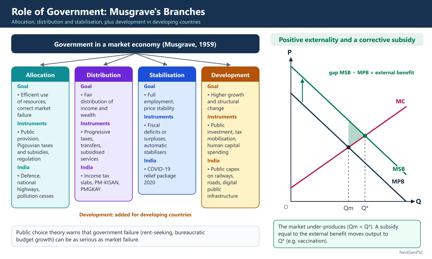
Richard Musgrave, The Theory of Public Finance (1959), divided the economic role of government into three branches: allocation (correcting market failures such as public goods and externalities), distribution (adjusting income and wealth to what society considers fair) and stabilisation (maintaining full employment and price stability). In developing countries a fourth role, development, is added: raising savings and investment, building infrastructure and human capital. Public choice theory warns that government failure can be as serious as market failure.
In simple words
Markets are good at producing mobiles and clothes, but they fail to supply things like street lights, clean air or vaccination for all.
A street light lights everyone's path whether they pay or not, so no private seller can charge for it; this is a public good.
So the government taxes and spends to fill such gaps, to reduce inequality, to steady the economy in booms and slumps and, in India, to speed up development.
UPSC asks you to explain Musgrave's branches with examples and weigh market failure against government failure.
1. Concepts and Definitions
Public finance: the study of government revenue, expenditure, borrowing and their effects on resource allocation, distribution and stability; Hugh Dalton, Principles of Public Finance (1922), called it a study of the income and expenditure of public authorities.
Market failure: a situation in which competitive markets do not reach a Pareto-efficient allocation; sources are public goods, externalities, market power, information asymmetry (Akerlof's 'lemons', 1970) and incomplete markets.
Pure public good: a good that is non-rival (one person's use does not reduce another's) and non-excludable (people cannot be prevented from using it); Paul Samuelson, 'The Pure Theory of Public Expenditure' (1954), gave the formal theory; examples: national defence, lighthouses, basic research.
Free-rider problem: because no one can be excluded, each person has an incentive to hide their true preference and let others pay, so private provision is too low.
Merit goods: Musgrave's term (1957) for goods society wants consumed more than individuals would choose (primary education, vaccination); demerit goods are the opposite (tobacco, alcohol).
Externality: a cost or benefit falling on third parties not reflected in prices; A.C. Pigou, The Economics of Welfare (1920), proposed taxes on negative and subsidies on positive externalities.
2. The Allocation Branch
Samuelson condition: efficient provision of a public good requires that the sum of all individuals' marginal rates of substitution equal the marginal rate of transformation: ΣMRS = MRT (for a private good, each MRS = MRT).
Lindahl equilibrium: Erik Lindahl (1919) proposed that each person pay a tax-price equal to his marginal benefit, so that the sum of tax-prices covers marginal cost; it fails in practice because people do not reveal preferences.
Correcting externalities: a Pigouvian tax equal to marginal external cost at the efficient output makes the producer internalise the cost; Ronald Coase, 'The Problem of Social Cost' (1960), showed that with clear property rights and low transaction costs private bargaining can reach efficiency without government (Coase theorem).
Natural monopoly and regulation: where average cost falls over the whole market range, government may own or regulate the firm (railways, electricity transmission), using marginal-cost pricing with subsidy or average-cost pricing.
Information and insurance: governments provide social insurance and regulate quality because of adverse selection and moral hazard.
3. The Distribution Branch
Purpose: markets distribute income according to factor ownership and productivity, which may be very unequal; society may want a different distribution on grounds of equity.
Tools: progressive income taxation, wealth and inheritance taxes, transfers (pensions, cash transfers), subsidised public services, and public employment programmes.
Value judgements: the choice depends on the social welfare function (utilitarian, Rawlsian maximin from John Rawls, A Theory of Justice, 1971); Musgrave separated distribution so that allocation decisions could be judged by efficiency alone.
Equity-efficiency trade-off: Arthur Okun, Equality and Efficiency: The Big Tradeoff (1975), described redistribution as carrying water in a 'leaky bucket' because taxes and transfers reduce incentives.
4. The Stabilisation Branch
Keynesian basis: aggregate demand can fall short of full employment output; government spending, taxes and deficits can fill the gap (J.M. Keynes, 1936).
Functional finance: Abba Lerner (1943) argued that fiscal policy should be judged by its effect on employment and prices, not by whether the budget balances.
Automatic stabilisers: progressive taxes and unemployment or employment-guarantee spending rise in slumps and fall in booms without new decisions.
Discretionary policy: deliberate changes in spending and taxes; subject to recognition, decision and implementation lags.
Supply stabilisation: in developing economies stabilisation also means steadying the supply and prices of essentials through buffer stocks, procurement, imports and export controls (in India the Food Corporation of India and price stabilisation funds).
5. The Development Role
Raising savings: taxation and public saving raise the investment rate needed for growth (the Harrod-Domar logic g = s/v); Nicholas Kaldor argued that developing countries need taxation to mobilise the surplus for development ('Will Underdeveloped Countries Learn to Tax?', 1963).
Big push and infrastructure: Rosenstein-Rodan (1943) and Nurkse stressed lumpy social overhead capital that only the state can provide; Hirschman stressed sequencing.
Human capital: public spending on health and education has high social returns (T.W. Schultz, 1961; endogenous growth theory).
Indian approach: planned public investment under the Mahalanobis strategy (Second Plan, 1956–61), and in recent years high public capital expenditure (Union capex budgeted at ₹11.2 lakh crore in 2025–26).
6. Government Failure and Public Choice
Public choice theory: James Buchanan and Gordon Tullock, The Calculus of Consent (1962), model politicians, voters and bureaucrats as self-interested; Buchanan received the Nobel Prize in 1986.
Sources of government failure: rent-seeking (Anne Krueger, 1974), budget-maximising bureaucrats (William Niskanen, 1971), short-term electoral cycles, capture of regulators by industry (George Stigler, 1971), and lack of information.
Implication: the case for intervention requires showing that the government can do better than the imperfect market, not just that the market fails (a point stressed by Coase and Demsetz's 'nirvana fallacy', 1969).
7. Diagrams to Draw
Public good demand (vertical summation): draw quantity on the horizontal axis and price on the vertical; draw individual demand curves D_A and D_B; add them vertically to get ΣD; the efficient quantity Q* is where ΣD cuts the marginal cost curve; contrast with horizontal summation for private goods.
Negative externality and Pigouvian tax: draw demand (marginal social benefit), private marginal cost (MPC) and social marginal cost (MSC) above it; the market produces Qm where MPC meets demand, the efficient output Q* is where MSC meets demand; shade the deadweight loss triangle; a tax equal to the vertical gap at Q* shifts MPC up to MSC.
Positive externality: draw marginal social benefit above marginal private benefit; the market under-produces; a subsidy equal to the external benefit corrects it (for example vaccination).
Musgrave branches chart: a box diagram with three branches, their goals, instruments and examples.
8. Examples and Applications
Allocation: national highways, defence and ISRO's space programme (public goods); Pollution taxes such as the former coal cess (clean energy cess, 2010) and vehicle scrappage incentives.
Distribution: progressive income tax, PM-KISAN cash transfer (2019) and free foodgrains under PMGKAY (extended for five years from January 2024).
Stabilisation: India's COVID-19 relief (Pradhan Mantri Garib Kalyan Package 2020 and Atmanirbhar packages) and the 2008–09 stimulus that raised the fiscal deficit.
Development: public capex on railways, roads and digital public infrastructure (Aadhaar, UPI), which crowds in private investment.
9. Using it in the Exam
10 marks: state Musgrave's three branches with one example each and add the development role for India.
15 marks: explain market failures (public goods with ΣMRS = MRT, externalities with a Pigouvian tax diagram).
20 marks: all four roles, the public-good and externality diagrams, government failure (Buchanan) and Indian examples with years.
Keywords: allocation, distribution, stabilisation, non-rivalry, non-excludability, free rider, merit goods, Pigouvian tax, Coase theorem, government failure.
Definition to quote: Samuelson (1954) defined a collective consumption good as one that all enjoy in common, in the sense that each individual's consumption leads to no subtraction from any other individual's consumption.
| Branch | Goal | Main instruments | Indian example |
|---|---|---|---|
| Allocation | Efficient use of resources; correct market failure | Public provision, Pigouvian taxes and subsidies, regulation | Defence, national highways, pollution cesses |
| Distribution | Fair distribution of income and wealth | Progressive taxes, transfers, subsidised services | Income tax slabs, PM-KISAN, PMGKAY |
| Stabilisation | Full employment, price stability | Fiscal deficits or surpluses, automatic stabilisers | COVID-19 relief package 2020 |
| Development | Higher growth and structural change | Public investment, tax mobilisation, human capital spending | Public capex on railways, roads, digital public infrastructure |
Mains points
- Start with Musgrave (1959) and his three branches; add development as the fourth role for developing countries such as India.
- Use the Samuelson condition ΣMRS = MRT and the vertical summation diagram for public goods; it differentiates a strong answer.
- For externalities, draw MPC and MSC with the Pigouvian tax, then mention the Coase theorem as an alternative.
- Balance the answer with government failure (Buchanan-Tullock, Krueger, Niskanen) and the 'nirvana fallacy'.
- Give Indian examples with years: PMGKAY extension (2024), public capex push, COVID-19 package (2020).
- Common mistake: calling every government-provided good a public good; education and health are merit goods because they are rival and excludable.
Did you know?
- The lighthouse was the textbook example of a public good until Coase (1974) showed that many British lighthouses were privately built and financed by fees collected at ports.
Taxation: Sources of Revenue, Forms, Incidence and Effects
Governments raise revenue through taxes (direct and indirect), non-tax revenue (fees, dividends, RBI surplus) and capital receipts. A good tax system follows Adam Smith's canons (equality, certainty, convenience, economy) and a principle of fairness: benefit or ability to pay. The person who legally pays a tax (impact) may shift it; the final incidence depends on the relative elasticities of demand and supply, and every distorting tax causes an excess burden (deadweight loss) that rises with the square of the tax rate.
In simple words
Taxes are how the government pays for roads, police and schools; some are paid directly on income (direct taxes), others are hidden in prices like GST (indirect taxes).
The shopkeeper deposits GST, but you may end up paying it in a higher price: who finally bears a tax is its incidence.
Whoever cannot easily switch away, buyer or seller, ends up bearing more of the tax.
UPSC asks you to explain incidence with demand-supply diagrams and compare direct and indirect taxes.
1. Sources of Government Revenue
Tax revenue: compulsory payments without a direct quid pro quo; direct taxes (personal income tax, corporation tax, wealth and property taxes) and indirect taxes (GST, customs duties, excise on petroleum and tobacco).
Non-tax revenue: fees, fines, interest receipts, dividends and profits of public enterprises, RBI surplus transfer, spectrum and other licence charges.
Capital receipts: borrowings, recovery of loans and disinvestment proceeds; they create liabilities or reduce assets.
India's structure: the Constitution's Seventh Schedule divides tax powers; since 1 July 2017 GST (Article 246A, 101st Amendment, 2016) subsumes most indirect taxes of the Centre and states; the Centre's gross tax revenue in recent years is roughly 11–12% of GDP, and Centre plus states together raise roughly 17–18% of GDP.
2. Canons and Principles of Taxation
Adam Smith's four canons: The Wealth of Nations (1776): equality (in proportion to ability), certainty (not arbitrary), convenience (time and manner of payment) and economy (low cost of collection).
Later canons: productivity, elasticity (revenue grows with income), flexibility, simplicity and diversity (Bastable and others).
Benefit principle: tax according to benefits received from public services (Lindahl, Wicksell); suits user charges and tolls, not redistribution.
Ability-to-pay principle: tax according to capacity measured by income, wealth or consumption; horizontal equity (equals treated equally) and vertical equity (unequals treated unequally).
Equal sacrifice versions: J.S. Mill's equal absolute sacrifice, proportional sacrifice, and Edgeworth-Pigou equal marginal sacrifice (least aggregate sacrifice), which, with identical diminishing marginal utility of income, implies steeply progressive taxation.
Optimal taxation: Frank Ramsey (1927): to minimise excess burden, commodity tax rates should be inversely proportional to demand elasticities (inverse elasticity rule), which conflicts with equity because necessities are inelastic; James Mirrlees (1971) built the theory of the optimal income tax balancing equity and labour supply incentives.
3. Forms of Taxes
Direct versus indirect: a direct tax is borne by the person on whom it is imposed (income tax); an indirect tax is imposed on one person but intended to be shifted to another (GST, excise).
Progressive, proportional and regressive: average tax rate rises, stays constant or falls as income rises; indirect taxes on necessities tend to be regressive relative to income.
Specific versus ad valorem: a fixed amount per unit (excise on cigarettes per stick) versus a percentage of value (GST at 18%).
Lump-sum tax: fixed regardless of behaviour, so non-distorting; rarely feasible and inequitable.
Direct and indirect compared: direct taxes are equitable, progressive and elastic but have narrow base and evasion problems; indirect taxes have a wide base and are easier to collect but are regressive and inflationary.
4. Tax Incidence and Shifting
Impact, shifting and incidence: impact is the initial legal burden; shifting is passing it forward to buyers or backward to factor owners; incidence is the final money burden (Hugh Dalton); the effects are the resulting changes in output, prices and behaviour.
Old theories: the concentration theory of the Physiocrats (all taxes ultimately fall on land) and the diffusion theory (taxes spread through the economy, associated with Mansfield and Thiers); the modern theory uses demand and supply.
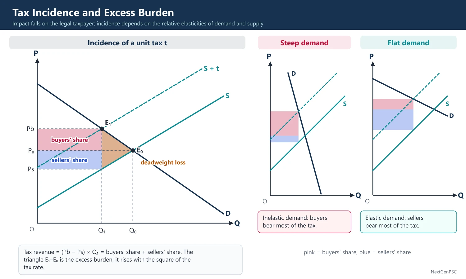
Partial equilibrium rule: share borne by buyers = Es/(Es + Ed) and share borne by sellers = Ed/(Es + Ed), where Ed and Es are absolute price elasticities; the less elastic side bears more.
Special cases: perfectly inelastic demand (life-saving drugs): buyers bear all; perfectly elastic demand: sellers bear all; perfectly inelastic supply (land): sellers bear all and the tax is capitalised into a lower land price.
Statutory incidence is irrelevant: in competitive markets, the economic incidence is the same whether the tax is levied on buyers or sellers.
Monopoly: with linear demand and constant marginal cost, a per-unit tax raises price by half the tax; with constant-elasticity demand price can rise by more than the tax.
General equilibrium incidence: Arnold Harberger (1962) showed that a tax on corporate capital is shifted to all capital owners through capital mobility, and possibly partly to labour.
5. Excess Burden (Deadweight Loss)
Meaning: the loss of welfare beyond the revenue collected, because the tax changes behaviour away from efficient choices.
Size: approximately the Harberger triangle, ½ × tax × fall in quantity; it rises with the square of the tax rate and with the elasticities, so a broad base with low rates is efficient.
Income tax versus excise tax: Hicks and Joseph (1939) used indifference curves to show that an income tax yielding the same revenue leaves the consumer on a higher indifference curve than an excise tax (it avoids substitution distortion); I.M.D. Little (1951) showed this depends on ignoring the work-leisure choice, since an income tax also distorts labour supply.
6. Economic Effects of Taxation
On work: a higher income tax has a substitution effect (leisure becomes cheaper, so work falls) and an income effect (lower income, so work rises); the net effect is ambiguous; the labour supply curve may bend backward.
On saving and investment: taxes on interest and capital gains reduce the return to saving; corporate taxes lower post-tax returns on investment; accelerated depreciation and investment allowances offset this.
On distribution: progressive direct taxes reduce inequality; regressive indirect taxes may increase it.
On prices and allocation: indirect taxes raise prices and shift demand between goods; cascading (tax on tax) distorts input choice, which GST's input tax credit reduces.
On growth: high marginal rates may discourage entrepreneurship and encourage evasion, which is the basis of the Laffer curve argument.
7. Diagrams to Draw
Incidence diagram: draw price on the vertical axis and quantity on the horizontal; draw demand D and supply S meeting at E0 (P0, Q0); shift supply up by the tax t to S + t; new equilibrium E1 at Pb (price paid by buyers) and Q1; drop down to S to get Ps (price received by sellers); the rectangle (Pb − P0) × Q1 is the buyers' share, (P0 − Ps) × Q1 the sellers' share; the triangle between Q1 and Q0 is the deadweight loss.
Elasticity comparison: draw two panels, one with steep demand (buyers bear most) and one with flat demand (sellers bear most).
Hicks-Joseph diagram: draw good X on the horizontal and good Y on the vertical; an excise on X pivots the budget line inward; an income tax with equal yield shifts the original line parallel through the post-excise consumption point; it touches a higher indifference curve.
Backward-bending labour supply: draw the wage on the vertical axis and hours on the horizontal; show labour supply rising and then bending back at high wages.
8. Examples and Applications
India's corporate tax cut (September 2019): base rate reduced to 22% for companies giving up exemptions and 15% for new manufacturing companies, to boost investment.
GST 2.0 (effective 22 September 2025): the GST Council moved most goods to two main slabs of 5% and 18%, with a special 40% rate for luxury and sin goods; an example of rate rationalisation to cut classification disputes and lower burden on mass consumption.
Personal income tax: the Union Budget 2025–26 raised the rebate so that income up to ₹12 lakh pays no tax under the new regime; the Income-tax Act, 2025, replacing the 1961 Act, applies from 1 April 2026.
Incidence of fuel taxes: fuel demand is price-inelastic in the short run, so excise and VAT on petrol and diesel fall largely on consumers.
9. Using it in the Exam
10 marks: define impact, incidence and shifting; state the elasticity rule with a small diagram.
15 marks: full incidence diagram with buyers' and sellers' shares and deadweight loss; special cases of elasticity.
20 marks: canons, principles, direct versus indirect taxes, incidence, excess burden, effects on work and saving, and Indian reforms (GST 2017 and GST 2.0 of 2025, corporate tax 2019, Income-tax Act 2025).
Keywords: canons of taxation, ability to pay, equal marginal sacrifice, incidence, shifting, elasticity, excess burden, Ramsey rule, progressive tax.
Formula to quote: buyers' share of a tax = Es/(Es + Ed).
| Basis | Direct taxes | Indirect taxes |
|---|---|---|
| Impact and incidence | On the same person | On different persons (shifted) |
| Equity | Progressive; follow ability to pay | Often regressive |
| Base and collection | Narrow base; evasion possible | Wide base; easier collection |
| Effect on prices | Not directly inflationary | Raise prices |
| Indian examples | Personal income tax, corporation tax | GST, customs duty, excise on fuel and tobacco |
| Case | Who bears the tax | Example |
|---|---|---|
| Demand perfectly inelastic | Buyers entirely | Life-saving drugs |
| Demand perfectly elastic | Sellers entirely | Small firm in a world market |
| Supply perfectly inelastic | Sellers entirely (tax capitalised) | Land |
| Demand less elastic than supply | Mostly buyers | Petrol, cigarettes |
| Supply less elastic than demand | Mostly sellers | Perishable farm produce at harvest |
Mains points
- Distinguish impact, shifting, incidence and effects at the start; examiners check this vocabulary.
- Always draw the incidence diagram with Pb, Ps, the tax wedge and the deadweight loss triangle.
- State the elasticity rule as a formula and illustrate special cases (land, life-saving drugs).
- Discuss Ramsey's inverse elasticity rule and its conflict with equity, a favourite analytical point.
- Bring in the Hicks-Joseph versus Little debate on direct versus indirect taxes for 15–20 mark questions.
- Indian illustrations: GST 2017 and GST 2.0 (2025), corporate tax cut (2019), Income-tax Act 2025.
- Common mistake: saying the party on whom the tax is legally imposed always bears it.
Did you know?
- Memory trick for incidence: 'The one who can run away escapes the tax.' The more elastic side (buyers or sellers who can switch) bears less.
Subsidies, Limits to Taxation and Tax Reform
A subsidy is a negative tax: it lowers the price paid by buyers or raises the price received by sellers, and its benefit is shared according to elasticities, with a deadweight loss unless it corrects an externality. Subsidies are justified for merit goods and positive externalities but can be costly, poorly targeted and distorting. Taxation also has limits: taxable capacity (Dalton, Findlay Shirras, Colin Clark) and the Laffer curve, beyond whose peak higher rates reduce revenue. Tax reform in India, from the Chelliah Committee (1991) to GST (2017) and GST 2.0 (2025), has aimed at broad bases, moderate rates and simpler administration.
In simple words
A subsidy is money or a price cut the government gives so that people can buy something cheaply, like LPG cylinders, fertiliser or rice from ration shops.
It works like a discount coupon paid by taxpayers: it helps the poor, but if given to everyone it costs a lot and can be misused.
Taxes also cannot rise forever; beyond a point people work less or hide income, so revenue falls.
UPSC asks about the effects of subsidies, cash versus in-kind transfers, the Laffer curve and India's tax reforms.
1. Concepts and Definitions
Subsidy: a payment by government that reduces the cost of producing or buying a good below its market cost; it may be explicit (budgeted cash) or implicit (under-pricing of public services, tax expenditures).
Forms: producer subsidies (input subsidies on fertiliser, power and water to farmers), consumer subsidies (food under the public distribution system, LPG), export subsidies, interest subsidies, and transfers in cash or in kind.
Merit and non-merit subsidies: a classification used by the NIPFP study Government Subsidies in India (D.K. Srivastava and others, 1997): merit subsidies go to goods with large external benefits (primary education, health, sanitation); non-merit subsidies go to goods with mostly private benefits; the study estimated total explicit and implicit subsidies at about 14% of GDP for 1994–95, most of them non-merit.
Tax expenditure: revenue forgone through exemptions, deductions and concessions; India's Union Budget publishes a statement of revenue impact of tax incentives each year.
2. Economic Effects of Subsidies
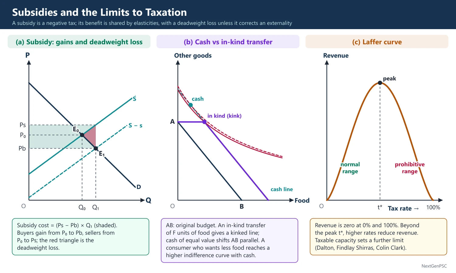
Price and quantity: a per-unit subsidy shifts supply down by the subsidy amount; buyers pay less, sellers receive more, and quantity rises.
Incidence of benefit: buyers' share = Es/(Es + Ed), sellers' share = Ed/(Es + Ed); a subsidy on a good with inelastic supply mostly benefits the owners of the scarce input (for example land rents rise).
Deadweight loss: the subsidy cost exceeds the gain to consumers and producers by a triangle, because units are produced whose cost exceeds their value to buyers.
Justified cases: positive externalities (vaccination, R&D, clean energy), merit goods, infant industries, and protecting the poor from price shocks.
Problems: fiscal burden, leakages and poor targeting (benefits captured by the non-poor), distortion of input use (overuse of urea and groundwater because power is free), environmental damage, and political difficulty of withdrawal.
3. Cash versus In-Kind Transfers
Standard result: for the same budget cost, a cash transfer leaves the recipient on an indifference curve at least as high as an in-kind transfer, because it allows free choice.
When they are equal: if the recipient would anyway consume more than the in-kind amount (an inframarginal transfer), the two are equivalent.
Case for in-kind: paternalism and merit goods (society cares about nutrition, not just utility), self-targeting (coarse grains attract only the poor), protection against inflation, and intra-household control (food reaches women and children).
India's shift: Direct Benefit Transfer (from 1 January 2013) and the JAM trinity (Jan Dhan, Aadhaar, Mobile), named in the Economic Survey 2014–15, moved LPG (PAHAL, 2014–15), scholarships and PM-KISAN (2019) to cash; food remains largely in kind, with free grain under PMGKAY.
4. Limits to Taxation
Taxable capacity: Hugh Dalton distinguished absolute taxable capacity (the maximum that can be taken without harmful effects on the economy) from relative capacity (fair shares between regions or groups); G. Findlay Shirras defined it as the limit beyond which further taxation reduces productive capacity.
Colin Clark's limit: Colin Clark (1945) argued that taxation above about 25% of national income would cause inflation through pressure on costs; later experience (many European countries above 40%) showed no fixed limit exists.
Determinants: level and distribution of income, size of the informal sector, tax morale and compliance, efficiency of administration, use of tax revenue (if spent productively capacity rises), political acceptance and international tax competition.
Laffer curve: associated with Arthur Laffer (1974); tax revenue is zero at 0% and at 100% tax rates, so it reaches a maximum at some intermediate rate t*; above t* cutting rates raises revenue; the idea is old (Ibn Khaldun, 14th century; Keynes also noted it).
Evidence on Laffer: most economists find developed economies are below the peak for average rates; very high top marginal rates (above roughly 70%) can be on the wrong side; India's experience after cutting the top personal income tax rate from 97.75% (early 1970s) suggested better compliance (debated).
Tax competition: mobile capital limits corporate tax rates; the OECD/G20 Inclusive Framework agreed in October 2021 on a two-pillar solution, including a 15% global minimum corporate tax (Pillar Two).
5. Tax Reform: Principles and Indian Experience
Principles: broad base and low rates, neutrality, simplicity, fewer exemptions, taxing consumption at destination, input tax credit to end cascading, and use of technology to widen the base.
Raja Chelliah Tax Reforms Committee (1991–93): recommended lower and fewer income tax rates, a lower corporate tax rate, a broader base, reduction of customs duties and a move towards VAT.
Earlier steps: MODVAT (1986), CENVAT (2000) and state VAT (from April 2005) gave input credits and reduced cascading.
Vijay Kelkar Task Forces (2002): on direct and indirect taxes: raise the exemption limit, cut exemptions, use technology (Tax Information Network, PAN); the Kelkar Task Force on the FRBM (2004) proposed a national GST.
Direct Taxes Code (2009–10 drafts): proposed to replace the Income-tax Act, 1961; it lapsed; the idea was revived as the Income-tax Act, 2025, which applies from 1 April 2026.
Tax Administration Reform Commission (Parthasarathi Shome, 2014): recommended a taxpayer-centric, unified administration.
GST (1 July 2017): 101st Constitutional Amendment (2016); destination-based dual GST with a GST Council; GST 2.0 from 22 September 2025 simplified rates to mainly 5% and 18% plus a 40% special rate.
Recent direct tax reforms: corporate tax cut (2019), optional new personal tax regime (2020, default from 2023–24), faceless assessment (2020), and the zero-tax limit of ₹12 lakh under the new regime (Budget 2025–26).
6. Diagrams to Draw
Subsidy diagram: draw demand D and supply S meeting at E0; shift supply down by the subsidy s to S − s; new equilibrium E1 at a lower buyer price Pb and higher quantity Q1; the seller price Ps is on the original S above Q1; the subsidy cost is the rectangle (Ps − Pb) × Q1; show the consumers' gain, producers' gain and the deadweight loss triangle between Q0 and Q1.
Cash versus in-kind: draw food on the horizontal axis and other goods on the vertical; the original budget line AB; an in-kind transfer of F units shifts the line right by F but with a vertical segment (kinked line); a cash transfer of equal value shifts the whole line parallel; show a consumer who reaches a higher indifference curve with cash.
Laffer curve: draw the tax rate (0 to 100%) on the horizontal axis and revenue on the vertical; an inverted U with a peak at t*; mark the normal range (left) and the prohibitive range (right).
7. Examples and Applications
Fertiliser subsidy: fixed urea prices with variable subsidy and nutrient-based subsidy (2010) for P and K fertilisers led to imbalanced use (excess nitrogen); neem-coated urea (2015) reduced diversion.
Petroleum: petrol was deregulated in June 2010 and diesel in October 2014, cutting subsidy burden; LPG subsidy moved to DBT (PAHAL).
Food: the National Food Security Act, 2013 covers up to 75% of the rural and 50% of the urban population; the Shanta Kumar Committee (2015) recommended restructuring the FCI and reducing coverage and moving to cash transfers.
World: fuel subsidy reforms in Indonesia (2015) and Iran's cash transfer reform (2010) show the role of compensation in making reform politically feasible.
8. Using it in the Exam
10 marks: define a subsidy, show its effect in a demand-supply diagram and give one Indian example.
15 marks: effects of subsidies with the welfare analysis plus cash versus in-kind debate and India's DBT.
20 marks: limits to taxation (taxable capacity, Laffer curve, tax competition) and tax reform in India from Chelliah to GST 2.0 and the Income-tax Act 2025.
Keywords: merit and non-merit subsidies, tax expenditure, deadweight loss, targeting, DBT, JAM, taxable capacity, Laffer curve, broad base low rate, input tax credit.
Point to quote: Colin Clark's 25% limit to taxable capacity has been refuted by experience; taxable capacity depends on how revenue is used.
| Year | Reform | Main change |
|---|---|---|
| 1986 | MODVAT | Credit for excise paid on inputs |
| 1991–93 | Chelliah Tax Reforms Committee | Fewer, lower rates; broader base; lower customs duties |
| 2002 | Kelkar Task Forces | Fewer exemptions; technology-based administration |
| 2005 | State VAT | Replaced sales tax with input credit in states |
| 2017 | GST | Destination-based dual GST; GST Council |
| 2019 | Corporate tax cut | 22% base rate; 15% for new manufacturing firms |
| 2025 | GST 2.0 (from 22 September) | Mainly 5% and 18% slabs; 40% special rate |
| 2026 | Income-tax Act, 2025 (from 1 April) | Replaces the Income-tax Act, 1961 |
Mains points
- Treat a subsidy as a negative tax and reuse the incidence logic and diagram; show the deadweight loss explicitly.
- Classify subsidies (merit and non-merit, explicit and implicit) using the NIPFP framework.
- In cash versus in-kind answers, give the indifference curve result and then the arguments for in-kind (paternalism, self-targeting, inflation protection).
- For limits to taxation, define taxable capacity (Dalton, Shirras), critique Colin Clark's 25% limit and draw the Laffer curve.
- For tax reform, present a chronology (Chelliah, Kelkar, VAT, GST 2017, GST 2.0 2025, Income-tax Act 2025) and principles (broad base, low rates).
- Common mistake: presenting the Laffer curve as proof that tax cuts always raise revenue; it only applies above the revenue-maximising rate.
Did you know?
- Arthur Laffer is said to have sketched his curve on a restaurant napkin in 1974 for Dick Cheney and Donald Rumsfeld; Jude Wanniski popularised the story and the name.
Public Borrowing, Crowding Out and Limits to Debt
Governments borrow when spending exceeds revenue. Whether public debt is a burden depends on who holds it, what it finances and the gap between the interest rate (r) and the growth rate (g): the debt ratio is stable if r is less than g and primary deficits are modest (Domar, 1944). Borrowing may crowd out private investment by raising interest rates, or may have no effect if households save for future taxes (Ricardian equivalence, Barro 1974), and in a slump public investment may crowd in private investment. India's fiscal anchor shifted from 2026–27 to a central debt target of 50 ± 1% of GDP by 2030–31.
In simple words
When the government spends more than it earns, it borrows by selling bonds; the total of past borrowing is public debt.
Like a family taking a home loan: borrowing is fine if income grows faster than the interest, but dangerous if interest keeps piling up.
Heavy government borrowing can also make loans costlier for businesses, which is called crowding out.
UPSC asks about the burden of debt, crowding out with IS-LM, Ricardian equivalence and how much debt India can safely carry.
1. Concepts and Definitions
Public debt: the stock of outstanding government liabilities arising from past borrowing; internal (owed to residents) or external (owed to foreigners), marketable (bonds, treasury bills) or non-marketable (small savings, provident funds).
Deficit measures: fiscal deficit = total expenditure − (revenue receipts + non-debt capital receipts), equal to the borrowing requirement; primary deficit = fiscal deficit − interest payments; revenue deficit = revenue expenditure − revenue receipts.
Crowding out: the reduction in private spending (especially investment) caused by an increase in government spending or borrowing, mainly through higher interest rates; crowding in is the opposite.
Ricardian equivalence: the proposition that, for a given path of government spending, financing by debt or by taxes has the same effect on demand, because rational households save the tax cut to pay future taxes; stated by Robert Barro, 'Are Government Bonds Net Wealth?' (Journal of Political Economy, 1974); named after David Ricardo, who discussed it but doubted it held in practice.
2. The Burden of Public Debt: Debate
Classical view: Adam Smith and Ricardo saw public debt as wasteful, diverting savings from productive capital to unproductive spending.
Keynes and Lerner: Abba Lerner (1948) argued that internal debt is no burden on the nation as a whole because 'we owe it to ourselves': interest is a transfer from taxpayers to bondholders; external debt is a real burden because repayment transfers resources abroad.
Buchanan's challenge: James Buchanan, Public Principles of Public Debt (1958), argued that the burden falls on future generations who must pay taxes to service debt from which they did not choose to benefit.
Life-cycle view: Bowen, Davis and Kopf (1960) showed that if the current generation sells bonds before retiring and consumes the proceeds, the burden passes to the next generation.
Modigliani (1961): the real burden is the smaller capital stock inherited by future generations when debt displaces private capital (crowding out); debt that finances productive public capital leaves no net burden.
Other burdens: distortion from taxes needed to pay interest (excess burden), transfer from taxpayers to richer bondholders (regressive), and loss of fiscal flexibility.
3. Crowding Out in the IS-LM Model
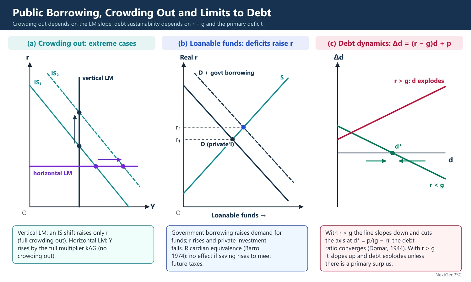
Mechanism: a bond-financed rise in G shifts IS to the right; higher income raises money demand; with a fixed money supply the interest rate rises; higher r reduces private investment; the final rise in Y is smaller than the simple multiplier would give (ΔY = kΔG at constant r).
Degree depends on slopes: full crowding out when LM is vertical (classical case: money demand not interest-sensitive) or IS is very flat (investment very interest-sensitive); zero crowding out when LM is horizontal (liquidity trap) or investment is interest-inelastic.
Accommodation: if the central bank expands money to hold r constant (monetisation), crowding out disappears, but inflation risk rises.
Wealth effects: Blinder and Solow (1973) noted that bonds held as wealth raise money demand (shifting LM left, more crowding out) and consumption (shifting IS right).
Open economy: under floating rates and capital mobility, higher interest rates attract capital, the currency appreciates and net exports fall (Mundell-Fleming); crowding out works through the trade balance.
Crowding in: in a slump with idle resources, or when public investment in infrastructure raises the productivity of private capital, public spending can raise private investment (accelerator effect; Aschauer, 1989, on public capital).
4. Ricardian Equivalence: Conditions and Critique
Required assumptions: infinitely-lived or altruistic households linked by bequests, perfect capital markets with no borrowing constraints, lump-sum taxes, rational foresight, and the same interest rate for government and households.
Critique: many households are liquidity-constrained (they spend tax cuts), people are myopic, taxes are distortionary, and the population grows (new taxpayers share the burden); empirical evidence supports at most partial Ricardian behaviour.
Implication if true: deficits do not raise interest rates or crowd out investment, and fiscal policy has no demand effect.
5. Debt Dynamics and Sustainability
Debt accumulation equation: Δd ≈ (r − g)·d + p, where d is the debt-to-GDP ratio, r the nominal interest rate on debt, g nominal GDP growth and p the primary deficit as a share of GDP.
Domar's condition: Evsey Domar, 'The Burden of the Debt and the National Income' (1944): if the government runs a constant deficit ratio b and nominal income grows at g, the debt ratio converges to d* = b/g; debt is sustainable as long as the economy grows.
Debt-stabilising primary balance: p* = −(r − g)·d; if r is less than g, a country can run a small primary deficit and keep d stable; if r exceeds g, it needs a primary surplus.
Olivier Blanchard (2019): in his presidential address 'Public Debt and Low Interest Rates' he argued that when r is persistently below g, the fiscal cost of debt is low (debated after interest rates rose in 2022–23).
Limits to borrowing: debt becomes unsustainable when markets doubt repayment, raising risk premiums and r (self-fulfilling crises); external and foreign-currency debt raise risk ('original sin', Eichengreen and Hausmann, 1999).
Debt thresholds: Reinhart and Rogoff, 'Growth in a Time of Debt' (2010), reported that growth falls sharply above 90% of GDP; Herndon, Ash and Pollin (2013) found coding and weighting errors and much weaker results; the existence of a universal threshold is debated.
Methods of debt redemption: sinking fund, conversion to lower interest rates, surplus budgets, capital levy, growth, inflation (erodes real debt) and, in extreme cases, repudiation or restructuring.
6. Diagrams to Draw
IS-LM crowding out: draw IS1 and LM in (Y, r) space meeting at E1 (Y1, r1); shift IS to IS2 by kΔG horizontally; mark Y3 = Y1 + kΔG at constant r1; the new equilibrium E2 is at Y2 (less than Y3) and r2 (higher); label the distance Y3 − Y2 as crowding out.
Extreme cases: a vertical LM (full crowding out: IS shift raises only r) and a horizontal LM (zero crowding out: Y rises by the full multiplier).
Loanable funds diagram: draw the real interest rate on the vertical axis and loanable funds on the horizontal; government borrowing shifts demand right (or reduces national saving, shifting supply left); the interest rate rises and private investment falls.
Debt dynamics phase line: draw d on the horizontal axis and Δd on the vertical; Δd = (r − g)d + p is a straight line; if r is less than g it slopes down and cuts the axis at a stable d*; if r exceeds g it slopes up and d explodes.
7. Examples and Applications
India's debt targets: the FRBM Review Committee (N.K. Singh, 2017) recommended general government debt of 60% of GDP (40% Centre, 20% states); from 2026–27 the Union Budget uses debt as the fiscal anchor, with central government debt budgeted at 55.6% of GDP for 2026–27 (56.1% in 2025–26 RE) and a target of 50 ± 1% by 2030–31; the fiscal deficit is budgeted at 4.3% of GDP for 2026–27.
Features reducing India's risk: debt is mostly domestic, rupee-denominated and long-dated, and nominal growth has usually exceeded the effective interest rate.
Crowding out in India: high government borrowing and the SLR historically pre-empted bank funds (financial repression); the 1980s fiscal expansion preceded the 1991 crisis.
World: the euro area sovereign debt crisis (Greece, 2010–12) shows limits to borrowing without a national central bank; Japan carries debt above 200% of GDP with low interest rates because it is held domestically.
8. Using it in the Exam
10 marks: define crowding out, show it on IS-LM in a few lines and name the extreme cases.
15 marks: burden of debt debate (Lerner, Buchanan, Modigliani) or Ricardian equivalence with conditions and critique.
20 marks: debt dynamics equation, Domar's condition, limits to borrowing, thresholds debate and India's new debt anchor with figures for 2026–27.
Keywords: fiscal deficit, primary deficit, crowding out, crowding in, Ricardian equivalence, r − g, debt sustainability, Domar condition, financial repression.
Quotation: Lerner's phrase that internal public debt is something 'we owe to ourselves'.
| View | Economist and year | Main argument |
|---|---|---|
| Classical | Smith (1776), Ricardo (1817) | Debt diverts savings from productive capital |
| Functional finance | Lerner (1943, 1948) | Internal debt is owed to ourselves; no national burden |
| Intergenerational | Buchanan (1958) | Future taxpayers bear the burden |
| Capital stock | Modigliani (1961) | Burden = lower capital stock inherited if debt crowds out capital |
| Ricardian equivalence | Barro (1974) | Debt and taxes equivalent; no effect on demand |
| Sustainability | Domar (1944); Blanchard (2019) | Debt ratio stable if growth exceeds interest rate |
Mains points
- Draw the IS-LM crowding-out diagram and label the gap between the multiplier shift and the actual rise in Y; this is the core of most questions.
- Show that the degree of crowding out depends on the slopes of IS and LM, and discuss crowding in under slack and infrastructure investment.
- Write the debt dynamics equation and Domar's result d* = b/g; examiners value the r − g condition.
- Present the burden of debt as a debate (Lerner vs Buchanan vs Modigliani) rather than a single view.
- Use India's current data: central debt 55.6% of GDP (2026–27 BE), target 50 ± 1% by 2030–31, fiscal deficit 4.3% (2026–27 BE).
- Mention the Reinhart-Rogoff controversy to show awareness that debt thresholds are contested.
- Common mistake: assuming Ricardian equivalence holds automatically; list its strict conditions.
Did you know?
- The Reinhart-Rogoff 90% debt threshold, widely cited to justify austerity, was challenged in 2013 by Thomas Herndon, a graduate student who found an Excel error while replicating it for a class assignment.
Public Expenditure: Growth Theories and Effects
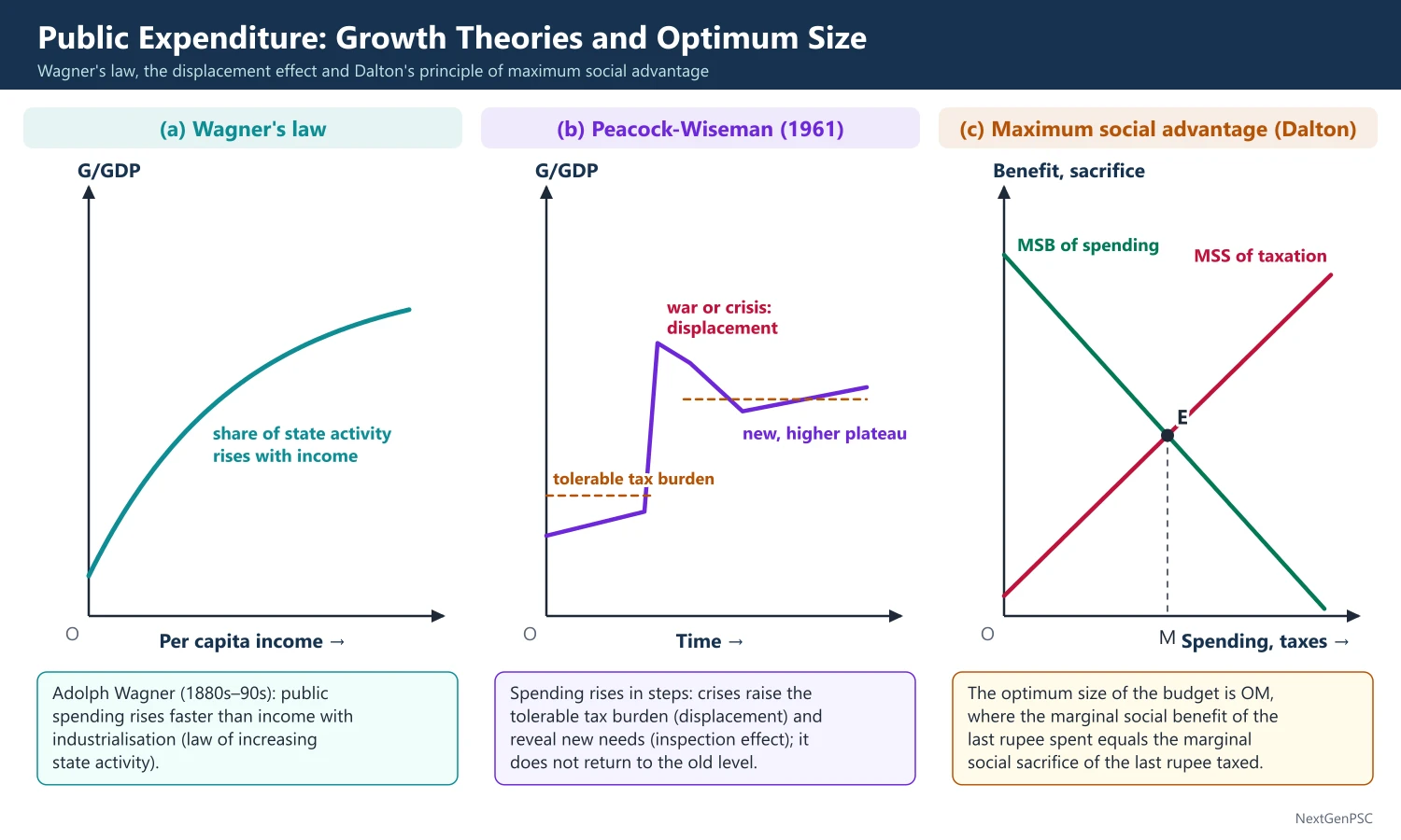
Public expenditure has grown faster than national income in most countries over the last century. Wagner's law (Adolph Wagner, 1880s–90s) explains this as a long-run rise in state activity with industrialisation; Peacock and Wiseman (1961) explain it as a step-wise displacement effect after wars and crises; Musgrave and Rostow link the composition of spending to stages of development; and Baumol's cost disease explains the rising relative cost of services. Spending affects production, distribution, stability (through the multiplier) and growth, and Dalton's principle of maximum social advantage sets the ideal size.
In simple words
Public expenditure is what the government spends on salaries, pensions, roads, schools, defence, subsidies and interest.
As a family gets richer it spends more on education and health; similarly, as countries develop, people demand more services from the state.
Government spending also creates jobs and income, which is why it is raised in a slowdown.
UPSC asks you to explain Wagner's law, the Peacock-Wiseman hypothesis and the effects of public spending with Indian examples.
1. Concepts and Classification
Public expenditure: spending by central, state and local governments on goods, services, transfers and investment.
Exhaustive versus transfer expenditure: A.C. Pigou distinguished spending that uses up real resources (salaries, roads) from transfers that redistribute purchasing power (pensions, interest, subsidies).
Revenue versus capital expenditure: revenue spending does not create assets (salaries, interest, subsidies); capital spending creates assets or reduces liabilities (roads, loans to states, debt repayment).
Developmental versus non-developmental: social and economic services versus defence, administration and interest.
India's budget classification: the plan/non-plan distinction was abolished from 2017–18 (following the C. Rangarajan Committee on efficient management of public expenditure, 2011); spending is now shown as revenue and capital, and by Centre's schemes, centrally sponsored schemes and establishment expenditure.
2. Wagner's Law of Increasing State Activity
Statement: Adolph Wagner (German economist, writing in the 1880s and 1890s) observed that as per capita income rises with industrialisation, the public sector grows faster than the economy, so the share of public spending in GDP rises.
Reasons given: (i) administrative and protective functions expand with urbanisation and complexity (law, order, regulation); (ii) cultural and welfare services such as education and health are income-elastic ('luxury' goods); (iii) natural monopolies and large-scale investment need state ownership or control.
Formal versions: economists test it as an income elasticity of public spending above one, using forms such as G = f(GDP), G/N = f(GDP/N) (Gupta) and G/GDP = f(GDP/N) (Musgrave).
Criticisms: it is a historical generalisation with no theory of political choice; it ignores wars and crises; causality may run from spending to income (the Keynesian view); evidence is mixed, stronger for developing countries in early stages; studies on India give mixed results depending on period and method.
3. Peacock-Wiseman Hypothesis
Source: Alan Peacock and Jack Wiseman, The Growth of Public Expenditure in the United Kingdom (1961), based on UK data from 1890 to 1955.
Core idea: government spending is limited by the 'tolerable burden of taxation' accepted by citizens; in normal times this changes slowly, so spending grows smoothly.
Displacement effect: wars and social upheavals force higher spending and taxes; people accept a higher tax tolerance, and after the crisis spending does not return to the old level, so it rises in steps.
Inspection effect: crises reveal social problems (poverty, health) that citizens then want government to solve.
Concentration effect: the central government's share of public spending rises relative to local governments during crises.
Criticisms: step increases are less clear in countries without major wars; the post-1970s growth of welfare spending happened without wars; it explains timing better than long-run level.
4. Other Theories of Expenditure Growth
Musgrave-Rostow development model: in early stages of development public investment in social overhead capital (roads, power, education) is a high share; in the middle stage public investment complements growing private investment; in the mature stage spending shifts to welfare, health and transfers (Musgrave, 1969; Rostow, 1971).
Baumol's cost disease: William Baumol, 'Macroeconomics of Unbalanced Growth' (American Economic Review, 1967): productivity in services such as education, health and administration grows slowly while wages follow the productive sectors, so the relative cost of public services rises over time.
Public choice explanations: budget-maximising bureaucrats (Niskanen, 1971), interest groups, fiscal illusion (taxes hidden in prices), and the median voter demanding redistribution when income is unequal (Meltzer and Richard, 1981).
Opposite view: Anthony Downs (1960) and J.K. Galbraith, The Affluent Society (1958), argued that public goods are under-supplied because their benefits are less visible ('private affluence and public squalor').
5. Principle of Maximum Social Advantage
Statement: Hugh Dalton (and Pigou) held that public finance is best when the marginal social benefit of the last rupee of public spending equals the marginal social sacrifice of the last rupee of taxation.
Logic: the marginal social benefit of public spending falls as spending rises, and the marginal social sacrifice of taxation rises; the optimal size is where the two curves cross.
Limits: benefits and sacrifices cannot be measured objectively; it ignores borrowing and the timing of benefits; but it gives the logic for cost-benefit analysis.
6. Effects of Public Expenditure
On production: Dalton noted effects on the ability to work, save and invest (health and education raise ability), the willingness to work and save (transfers may reduce it), and the diversion of resources between sectors and regions.
On distribution: progressive spending (free health, education, food) raises the real income of the poor more than proportionately; subsidies captured by the rich are regressive.
On stabilisation: the government expenditure multiplier is k = 1/(1 − c) in a simple model (or 1/(1 − c(1 − t) + m) with taxes and imports); Trygve Haavelmo (1945) showed that the balanced budget multiplier is 1 (equal rise in G and lump-sum T raises Y by the same amount).
On growth: Robert Barro (1990) modelled productive public spending as an input to private production, with growth first rising and then falling as the share of such spending increases; David Aschauer (1989) linked the US productivity slowdown to lower public infrastructure investment.
Composition matters: capital expenditure has a larger multiplier than revenue spending; RBI and other studies for India estimate a capex multiplier well above one and a revenue expenditure multiplier below one (estimates vary).
7. Diagrams to Draw
Wagner's law: draw per capita income on the horizontal axis and the share of public spending in GDP on the vertical; draw a rising curve.
Peacock-Wiseman: draw time on the horizontal axis and public spending as a share of GDP on the vertical; draw a line rising gently, jumping up at a war or crisis (displacement), then levelling at the new higher plateau; mark 'displacement', 'inspection' and the higher 'tolerable tax burden'.
Maximum social advantage: draw spending and taxation on the horizontal axis and benefit or sacrifice on the vertical; draw a downward-sloping MSB curve and an upward-sloping MSS curve; their intersection gives the optimum size OM.
Keynesian cross: draw the 45° line and the aggregate demand line C + I + G; a rise in G shifts the line up; income rises by kΔG.
8. Examples and Applications
India: the Union government's capital expenditure rose sharply after 2020–21 (budgeted at ₹11.2 lakh crore in 2025–26) to crowd in private investment and build infrastructure, an application of the development role and the capex multiplier.
COVID-19 displacement: spending on health, food (PMGKAY) and transfers rose sharply in 2020–21; some of it, such as free foodgrains, became permanent, consistent with the displacement effect.
Welfare states: public spending in many European countries rose from about 10% of GDP before 1914 to 40–50% after 1945, with sharp jumps at the two World Wars (supporting Peacock-Wiseman).
Expenditure reform in India: the Expenditure Management Commission (Bimal Jalan, 2014), outcome budgets (from 2005–06) and rationalisation of centrally sponsored schemes aim to improve the quality of spending.
9. Using it in the Exam
10 marks: state Wagner's law with reasons and one criticism.
15 marks: compare Wagner and Peacock-Wiseman with the step diagram.
20 marks: theories of growth of public spending, effects on production, distribution and stability with the multiplier, and India's capex push.
Keywords: Wagner's law, increasing state activity, displacement effect, inspection effect, concentration effect, tolerable tax burden, cost disease, maximum social advantage, balanced budget multiplier.
Statement to quote: Peacock and Wiseman argued that public spending rises in steps because social disturbances displace the tolerable level of taxation.
| Theory | Author and year | Core idea | Pattern predicted |
|---|---|---|---|
| Law of increasing state activity | Wagner (1880s–90s) | Industrialisation raises demand for state functions; income elasticity above 1 | Smooth long-run rise in G/GDP |
| Displacement effect | Peacock and Wiseman (1961) | Crises raise tolerable tax burden permanently | Step-wise rise |
| Development stages | Musgrave (1969), Rostow (1971) | Composition shifts from public investment to welfare | Changing mix over stages |
| Cost disease | Baumol (1967) | Slow productivity growth in services raises their relative cost | Rising cost share of public services |
| Public choice | Niskanen (1971); Meltzer-Richard (1981) | Bureaucrats and voters push budgets up | Over-expansion of government |
Mains points
- For Wagner's law, give the three reasons, a formal test (income elasticity of public spending above one) and criticisms.
- For Peacock-Wiseman, name all three effects (displacement, inspection, concentration) and draw the step diagram.
- Contrast the two theories: smooth versus step-wise growth, demand-side versus tax-tolerance explanations.
- Add the effects of spending using the multiplier and balanced budget multiplier (Haavelmo, 1945).
- Use India: capex push after 2020–21, end of the plan/non-plan distinction in 2017–18, COVID-19 as a displacement episode.
- Common mistake: writing Wagner's law as 'government spending grows with income'; it claims spending grows faster than income (share rises).
Did you know?
- Memory trick for Peacock-Wiseman: 'D-I-C' – Displacement (spending jumps), Inspection (problems seen), Concentration (Centre gains).
UPSC Previous Year Questions: Public Finance
From 2014 to 2026 UPSC asked 22 question parts (325 marks) from Public Finance in Paper I. Tax incidence and the effects of taxation (9 parts) dominate, followed by crowding out and public debt (5 parts); the role of government, subsidies and public expenditure make up the rest. Every question below has a model answer written to the UPSC word limit.
In simple words
Read the question and spend five minutes writing your own outline: definition, model or diagram, and conclusion.
Then read the model answer and tick what you missed: the economist's name, the diagram, the condition or the Indian example.
Rewrite one answer a day within the word limit (10 marks about 150 words, 15 marks about 200, 20 marks about 250) until the structure becomes a habit.
1. Role of Government in a Market Economy: Allocation, Distribution, Stabilisation and Development
Example 1 (UPSC 2026, 20 marks): Explain the instruments through which the government of any country tries to successfully carry out its three major roles namely, Allocation, Distribution and Stabilization.
Paper and question: Paper I, Q4(a)
Approach: Explain the three branches (Musgrave) and, for each, the fiscal and regulatory instruments used, with examples; end with the need for coordination.
Richard Musgrave, in The Theory of Public Finance (1959), divided the fiscal functions of government into three branches: allocation, distribution and stabilisation. Each corrects a different failure of the market and each uses its own instruments.
Allocation branch: markets under-supply public goods (non-rival, non-excludable), over-produce goods with negative externalities and under-produce merit goods. Instruments: direct provision financed by taxes (defence, roads, basic research); Pigouvian taxes and tradable permits for pollution (carbon taxes, the EU Emissions Trading System); subsidies for positive externalities (vaccination, education); regulation of natural monopolies and competition law; and public enterprises where private supply is absent.
Distribution branch: the market distributes income according to factor endowments, which society may judge unfair. Instruments: progressive income and wealth or inheritance taxes; transfer payments (pensions, unemployment benefits, cash transfers such as PM-KISAN in India); subsidised food under India's National Food Security Act, 2013; and public spending on health and education that equalises opportunity.
Stabilisation branch: the economy fluctuates around full employment. Instruments: discretionary fiscal policy (changes in spending and tax rates, public works in recessions), automatic stabilisers (progressive taxes, unemployment insurance), fiscal rules such as India's FRBM Act, 2003, and coordination with monetary policy.
In developing countries a fourth, development role is added: public investment in infrastructure, mobilisation of savings and planning to raise the growth rate.
The instruments interact: a progressive tax serves distribution and stabilisation at once, while a subsidy for equity may distort allocation. Musgrave therefore treated the branches as separate conceptual tasks so that each objective has an instrument, consistent with Tinbergen's rule that the number of instruments must equal the number of targets. Successful public finance needs coordination between the branches and between the fiscal and monetary authorities.
Example 2 (UPSC 2020, 10 marks): In the context of a developing economy, do you think that fiscal policy is more effective than monetary policy? Give reasons in support of your answer.
Paper and question: Paper I, Q5(d)
Approach: Take a reasoned position (fiscal policy is generally more effective in a developing economy), give structural reasons, then note the limits and the need for coordination.
In a developing economy fiscal policy is usually more effective than monetary policy, because the channels through which monetary policy works are weak.
First, monetary transmission is weak: financial markets are shallow, a large informal sector borrows from moneylenders, and investment is less sensitive to interest rates than to infrastructure and demand. In IS-LM terms the IS curve is steep, so a shift of LM changes output little.
Second, the main problems are structural: supply bottlenecks, unemployment and poverty. Public investment in roads, power and irrigation raises both demand and capacity, and the multiplier is high where the marginal propensity to consume is high.
However, fiscal policy has limits: large deficits, high public debt and recognition and implementation lags. Much inflation in India comes from food supply shocks, which neither policy cures quickly, and since 2016 the RBI's flexible inflation targeting has improved monetary credibility.
Hence fiscal policy is the stronger instrument for growth and development, while monetary policy is better for price stability; the two work best together.
Example 3 (UPSC 2019, 10 marks): Automatic stabilizers are supposed to mitigate cyclical fluctuations, but there exist limitations which dampen the effect of these stabilizers. Analyze.
Paper and question: Paper I, Q5(d)
Approach: Define automatic stabilisers and show how they work, then analyse the limitations that weaken them, especially in developing economies.
Automatic (built-in) stabilisers are budget features, such as progressive income tax and unemployment benefits, that change revenue and spending with the cycle without any new decision. In a recession revenue falls and transfers rise, so disposable income falls less than national income.
They lower the multiplier: with a proportional tax rate t, the multiplier becomes 1/[1 − c(1 − t)], smaller than 1/(1 − c), so a given shock moves output less.
Limitations: (i) they only dampen fluctuations and cannot restore full employment after a deep shock; (ii) they cause fiscal drag, as rising revenue slows the recovery; (iii) their strength depends on the size of government and the progressivity of taxes, and in India the income tax base is narrow, indirect taxes dominate and unemployment insurance is largely absent; (iv) the large informal sector lies outside the tax and transfer system.
Thus automatic stabilisers are a useful first line of defence, but they must be supplemented by discretionary fiscal and monetary policy.
2. Taxation: Sources of Revenue, Forms, Incidence and Effects
Example 4 (UPSC 2025, 15 marks): (i) Suppose that the market demand and supply functions are given by:
Qd = −500P + 5000
and Qs = 400P − 400
Find out the effects of imposition of specific sales tax of 18% on equilibrium price and quantity.
(ii) In a monopoly market, the demand and cost curves are given by:
p = 200 − 8q
and c = 25 + 10q
Suppose that the government imposes a tax of ₹10 per unit. How will equilibrium price and quantity be affected?
Paper and question: Paper I, Q4(b)
Approach: Solve both parts step by step: (i) find the pre-tax equilibrium, insert the tax as a wedge between the buyer's and the seller's price and compare; (ii) equate MR with MC before and after the per-unit tax.
(i) A sales tax drives a wedge between the price paid by buyers (P) and the price received by sellers (Ps); quantity is read from demand at P and from supply at Ps.
Step 1 (pre-tax): −500P + 5000 = 400P − 400, so 900P = 5400, P = ₹6 and Q = 5000 − 3000 = 2000 units.
Step 2 (tax of 18% on the seller's price, as with GST): P = 1.18 Ps. Then 5000 − 500P = 400(P/1.18) − 400, i.e. 5400 = P(500 + 338.98), so P = 6372/990 = ₹6.44 (approx.), Ps = 6.44/1.18 = ₹5.45, and Q = 5000 − 500 × 6.436 = 1782 units (approx.). Tax per unit = ₹0.98: buyers bear ₹0.44 and sellers ₹0.55.
Step 3 (if the 18% is read as a specific tax equal to 18% of the original price, t = ₹1.08 per unit): 5000 − 500P = 400(P − 1.08) − 400, so 900P = 5832, P = ₹6.48, Ps = ₹5.40 and Q = 1760 units.
In words: under either reading the price paid rises, the price received falls and quantity falls; the burden is split 4 : 5 between buyers and sellers because the burden ratio equals the ratio of the supply slope to the demand slope (400 : 500), i.e. the side with the less elastic curve bears more.
(ii) TR = 200q − 8q², so MR = 200 − 16q; MC = 10 because TC = 25 + 10q.
Step 4 (before tax): 200 − 16q = 10, so q = 11.875 and p = 200 − 8(11.875) = ₹105; profit = 1246.875 − 143.75 = ₹1103.1.
Step 5 (tax of ₹10 per unit): MC becomes 20, so 200 − 16q = 20, q = 11.25 and p = 200 − 90 = ₹110; tax revenue = ₹112.5 and profit falls to 1237.5 − 250 = ₹987.5.
In words: the monopolist's output falls from 11.875 to 11.25 and price rises by ₹5, exactly half the tax, which is the standard result for linear demand and constant marginal cost; the other half is borne by the monopolist. Unlike a competitive industry, the monopolist cannot pass on the whole tax because raising price further would reduce profit.
Example 5 (UPSC 2024, 10 marks): Show that ad valorem tax is preferable to specific sales tax from a firm's point of view in generating the same level of tax revenue.
Paper and question: Paper I, Q1(c)
Approach: Compare a specific tax and an ad valorem tax that raise the same revenue from a profit-maximising (monopoly) firm; prove the result with MR-MC reasoning and a diagram.
A specific tax t per unit raises the firm's marginal cost to MC + t; an ad valorem tax at rate τ takes a share of revenue, so net marginal revenue becomes (1 − τ)MR.
Let q₁ be output under the specific tax, where MR = MC + t, and let τ raise the same revenue at q₁, so τp = t. Since MR is less than p on a downward-sloping demand curve, τMR is less than t. Hence at q₁, net marginal revenue under the ad valorem tax, MR − τMR, exceeds MR − t = MC.
So the firm expands output beyond q₁: output is larger and price lower. At q₁ profit would be the same under both taxes, so profit at the chosen output must be higher, and since revenue also rises, an even lower rate gives equal yield.
Diagram: demand D and MR falling, MC rising; the specific tax shifts MC up parallel to MC + t, the ad valorem tax pivots MR down to (1 − τ)MR; the ad valorem equilibrium lies to the right of the specific-tax equilibrium.
Hence, for equal revenue, the firm earns more profit under the ad valorem tax and consumers pay less; under perfect competition, where MR = p, the two taxes are equivalent.
Example 6 (UPSC 2023, 15 marks): Tax burden is distributed between buyers and sellers in the ratio of elasticities of demand and supply. Explain.
Paper and question: Paper I, Q4(b)
Approach: Derive the incidence rule with the tax wedge (Δ prices in terms of elasticities), draw the diagram and illustrate the extreme cases.
The legal (impact) incidence of a tax falls on whoever pays it to the government, but its economic (effective) incidence depends on how prices adjust. In a competitive market the burden is shared in inverse proportion to the price elasticities: the more inelastic side bears more.
Let a small specific tax t be imposed. The buyer's price rises by ΔPd and the seller's price falls by ΔPs, with ΔPd + ΔPs = t. For the market to clear, the fall in quantity demanded must equal the fall in quantity supplied: Ed × (ΔPd/P) = Es × (ΔPs/P), where Ed is the absolute demand elasticity and Es the supply elasticity.
Hence ΔPd/ΔPs = Es/Ed, i.e. buyers' share/sellers' share = Es/Ed. Equivalently the buyers' share of the tax is Es/(Es + Ed) and the sellers' share is Ed/(Es + Ed). This rule goes back to Marshall's and Dalton's analysis of tax shifting.
Diagram: demand D and supply S in (Q, P) space with equilibrium E at P₀, Q₀; the tax shifts S up by t to S + t; new quantity Q₁; buyers pay P₁ above P₀ and sellers receive P₁ − t below P₀; the rectangle above P₀ is the buyers' burden and the one below is the sellers' burden; the triangle between is the deadweight loss.
Extreme cases: perfectly inelastic demand (Ed = 0) or perfectly elastic supply puts the whole burden on buyers; perfectly inelastic supply (land, Henry George's argument) or perfectly elastic demand puts it on sellers. Examples: excise on tobacco and petrol, whose demand is inelastic, falls mainly on consumers, while a tax on one brand among many close substitutes falls mainly on producers.
The rule holds for partial equilibrium and small taxes; in the long run supply is more elastic, so a larger share shifts to buyers.
Example 7 (UPSC 2022, 20 marks): State the canons of taxation. Do you think that direct taxes are less burdensome than indirect taxes in generating equal amount of tax revenue? Justify your answer.
Paper and question: Paper I, Q4(a)
Approach: List Adam Smith's four canons and the later ones briefly, then compare an income tax and an excise of equal yield with the indifference-curve proof, and qualify the conclusion.
Canons of taxation: Adam Smith, in The Wealth of Nations (1776), gave four canons: equality (tax in proportion to ability), certainty (amount and time not arbitrary), convenience (levied at a convenient time and manner) and economy (low cost of collection). Later writers such as Bastable added productivity, elasticity (revenue rising with income), flexibility, simplicity and diversity.
Direct versus indirect taxes: the classic welfare comparison (Hotelling, 1938; Joseph and Hicks, 1939) shows that a direct income tax is less burdensome than an indirect excise that raises the same revenue.
Diagram: goods X and Y on the axes, budget line AB, initial equilibrium E₀ on IC₀; an excise on X pivots the budget line inwards to AC, equilibrium E₁ on IC₁; draw a line A′B′ parallel to AB through E₁ (an income tax of the same yield, since the consumer pays the same amount at E₁); it touches a higher curve IC₂ at E₂, so welfare is higher under the income tax.
The reason is that the excise changes relative prices and adds a substitution effect, creating an excess burden, whereas an income tax has only an income effect on the choice between goods. Direct taxes can also be made progressive and so satisfy the canon of equality.
But the conclusion is not general. I.M.D. Little (1951) showed that an income tax also distorts the choice between work and leisure, so with leisure as a third good either tax may be superior. A uniform tax on all goods is equivalent to an income tax; Ramsey's rule favours higher indirect taxes on inelastic goods; and in developing countries indirect taxes are easier to collect and reach the informal sector, with lower administrative and compliance costs.
Hence direct taxes are less burdensome only in the narrow partial-equilibrium sense; a good tax system combines both, which is why India relies on income tax together with the GST.
Example 8 (UPSC 2021, 15 marks): If the government raises taxes on labour income and interest income, explain how potential GDP and economic growth are affected.
Paper and question: Paper I, Q8(a)
Approach: Use the supply-side (tax wedge) framework: a labour income tax affects labour supply and potential GDP; an interest income tax affects saving, investment and capital accumulation, hence growth; state the conditions.
Potential GDP is the output produced when labour is fully employed with the existing capital and technology; economic growth depends on how fast the capital stock, labour and technology expand. Factor-income taxes create a tax wedge between what employers or borrowers pay and what workers or savers receive.
Tax on labour income: labour demand depends on the pre-tax wage and labour supply on the after-tax wage. The tax lowers the after-tax wage; if the substitution effect dominates, workers supply fewer hours, so equilibrium employment falls.
Diagram: labour market with demand LD and supply LS; the tax shifts LS up by the tax to LS + tax; employment falls from L₀ to L₁; through the production function, lower employment gives lower potential GDP.
Tax on interest income: saving depends on the after-tax real interest rate. The tax lowers this return; if the substitution effect dominates, the supply of loanable funds shifts left, the pre-tax real interest rate rises and investment falls. A smaller flow of investment slows capital accumulation, so labour productivity and potential GDP grow more slowly; in Solow's model a lower saving rate lowers the steady-state level of income, and in endogenous growth models it can lower the long-run growth rate itself.
The size of the effect depends on elasticities: if labour supply is backward-bending or saving is income-dominated (target savers), the losses are smaller. The use of the revenue also matters: if it finances infrastructure or education, growth may rise.
Overall, higher taxes on labour and interest income tend to reduce potential GDP and growth, the core of the supply-side case for low marginal rates.
Example 9 (UPSC 2019, 15 marks): The role of income and substitution effect is crucial in producing backward bending labour supply curve when a tax is imposed on wages. Do you agree?
Paper and question: Paper I, Q3(a)
Approach: Agree, with qualification: use the income-leisure diagram to show that a wage tax has opposite substitution and income effects, and that a backward-bending supply arises when the income effect dominates.
Yes. A tax on wages lowers the net wage, and its effect on hours worked depends on two opposing forces, the substitution effect and the income effect, as in Hicks's analysis of labour supply.
The substitution effect: leisure becomes cheaper because an hour of leisure now costs less forgone net income, so the worker substitutes leisure for work and supplies fewer hours.
The income effect: the tax makes the worker poorer; since leisure is a normal good, he consumes less leisure and works more to maintain his income.
Diagram: leisure on the horizontal axis (maximum 24 hours) and income on the vertical axis; the budget line pivots down from the 24-hour point when the net wage falls; the worker moves from E₀ on IC₀ to E₁ on a lower curve; a compensated budget line parallel to the new one and tangent to IC₀ splits the move into the substitution effect (more leisure) and the income effect (less leisure).
If the substitution effect dominates, the tax reduces hours; if the income effect dominates, as at high wages or for target earners who must meet fixed commitments, the tax increases hours. Tracing hours against the net wage gives a labour supply curve that slopes upward at low wages and bends backward at high wages, where the income effect dominates.
Hence the backward-bending supply curve is purely a result of the relative strength of the two effects, which is why the effect of a wage tax on work effort is ambiguous in theory and an empirical question. Evidence suggests that prime-age men's hours respond little, while second earners respond more.
Example 10 (UPSC 2018, 20 marks): The burden of tax depends upon the elasticity of demand and supply of a commodity or service. Explain with suitable examples.
Paper and question: Paper I, Q4(c)
Approach: State the incidence rule (burden in inverse proportion to elasticities), show it with the tax-wedge diagram, then give examples for each combination of elasticities.
Tax incidence means the final resting place of the money burden of a tax. Whoever is legally liable, the burden is shared between buyers and sellers according to elasticities: buyers' share/sellers' share = Es/Ed, so the side that is less able to change its behaviour bears more.
The reason is that a tax creates a wedge t between the buyer's price and the seller's price. The side that can easily reduce its quantity (elastic) escapes by withdrawing; the side that cannot (inelastic) has to accept a worse price.
Diagram: two panels; in each, supply S shifts up by t to S + t. In panel (a) demand is steep (inelastic): the buyer's price rises almost by the full tax and the seller's price falls little. In panel (b) demand is flat (elastic): the buyer's price hardly rises and the seller's price falls by most of the tax. Shade the buyers' and sellers' burden rectangles.
Illustrations: (i) inelastic demand: excise duties on cigarettes, liquor and petrol and diesel in India are largely passed on to consumers, which is why these are favoured revenue sources. (ii) Elastic demand: a tax on one brand of soap or on one state's lottery is largely borne by the seller, because buyers switch to substitutes. (iii) Inelastic supply: a tax on land rent or on urban vacant land cannot be shifted and falls on owners. (iv) Elastic supply: in the long run, a tax on a competitive industry with constant costs falls wholly on consumers. (v) Labour: an employer payroll tax falls largely on workers when labour supply is inelastic.
Elasticities change over time, so incidence in the long run differs from the short run; market structure also matters, since a monopolist with linear demand and constant cost passes on only half of a unit tax.
Hence elasticity, not the legal point of collection, decides who really pays, which is why the GST Council and finance ministers judge goods by their demand elasticity when setting rates.
Example 11 (UPSC 2017, 10 marks): Distinguish between effective and differential tax incidence.
Paper and question: Paper I, Q5(a)
Approach: Define effective (economic) incidence against impact incidence, then Musgrave's differential incidence, and give an example of each.
Richard Musgrave (1959) defined incidence as the change in the distribution of real income caused by a change in budget policy, and distinguished several concepts of it.
Effective (economic) incidence is the final distribution of the burden after all shifting through prices, as distinct from impact incidence on the person legally liable. For example, GST is paid by the registered seller, but much of it is borne by consumers through higher prices.
Differential incidence is the change in distribution when one tax is replaced by another of equal yield, with public expenditure held constant. For example, replacing part of the income tax with an equal-yield sales tax shifts the burden towards poorer households, because the sales tax is regressive.
Thus effective incidence concerns the shifting of a single tax, while differential incidence compares two taxes with the budget size fixed, isolating the effect of the tax structure. Musgrave also defined absolute and balanced-budget incidence.
Differential incidence is the most useful concept for tax reform.
Example 12 (UPSC 2014, 10 marks): What do you understand by shifting of a tax? How does a monopolist succeed in shifting the burden of a tax under increasing marginal cost?
Paper and question: Paper I, Q2(c)
Approach: Define shifting (forward and backward), then show with MR-MC analysis that a monopolist with rising marginal cost shifts part of a unit tax, less than half under linear demand.
Shifting is the process by which the person legally liable for a tax passes its burden to others through price changes: forward to buyers through higher prices, or backward to input suppliers through lower prices.
A monopolist maximises profit where MR = MC. A lump-sum or profit tax leaves MR and MC unchanged and cannot be shifted. A specific tax t raises MC to MC + t, so the monopolist cuts output and raises price.
With linear demand p = a − bq and rising marginal cost MC = c + dq (d greater than 0), output is q = (a − c − t)/(2b + d), so price rises by Δp = bt/(2b + d), which is less than t/2; with constant MC (d = 0) it rises by exactly half the tax.
Diagram: demand D and MR falling, MC rising; the tax shifts MC up to MC + t; the new MR = MC point gives smaller output Q₁; price on the demand curve rises from P₀ to P₁ by less than t.
Thus under increasing marginal cost the monopolist shifts only part, less than half, of the tax, because marginal cost falls as output falls and absorbs part of it; the steeper the MC curve, the smaller the share shifted.
3. Subsidies, Limits to Taxation and Tax Reform
Example 13 (UPSC 2020, 20 marks): Discuss different forms of subsidies. Explain how perverse subsidies are detrimental to the economy and environment in the long run.
Paper and question: Paper I, Q8(c)
Approach: Classify subsidies (by form and by purpose), define perverse subsidies, and explain their long-run economic and environmental harm with Indian and global examples.
A subsidy is a payment or concession by government that lowers the price paid by a buyer or raises the price received by a producer. Subsidies are justified for merit goods, positive externalities and equity.
Forms: (i) direct cash transfers (DBT, PM-KISAN); (ii) price subsidies on consumption (food under NFSA, LPG) or inputs (fertiliser, power, irrigation water); (iii) production and export subsidies (production-linked incentives); (iv) interest subsidies and credit guarantees; (v) tax expenditures such as exemptions and concessions; (vi) in-kind transfers (mid-day meals); and (vii) implicit subsidies through under-priced public services. They may be explicit (budgeted) or implicit (hidden in low user charges).
Perverse subsidies, a term popularised by Norman Myers and Jennifer Kent (Perverse Subsidies, 2001), are subsidies that harm both the economy and the environment.
Economic harm: they distort relative prices, cause over-use of the subsidised input and create deadweight loss; they are regressive when richer users consume more (large farmers using more free power); they crowd out public investment, as input subsidies in Indian agriculture grew while public capital formation stagnated; and they become politically hard to withdraw.
Environmental harm: free or flat-rate electricity in Punjab and Haryana encourages over-pumping, and groundwater tables are falling; the bias towards urea has distorted the N:P:K ratio, degrading soil health; MSP procurement favouring rice and wheat locks water-intensive crops into dry regions; and fossil-fuel subsidies worldwide encourage emissions and delay the shift to renewables. Fishing subsidies drive over-fishing, which the WTO Agreement on Fisheries Subsidies (2022) addresses.
Reform lies in replacing price subsidies with targeted direct transfers, pricing inputs at closer to cost (as with petrol and diesel deregulation in 2010 and 2014), and redirecting savings to public investment and green technology.
Example 14 (UPSC 2015, 20 marks): "Subsidies have both positive and negative impacts on the economy." Explain this statement and illustrate your answer with Indian experience.
Paper and question: Paper I, Q4(b)
Approach: Explain the positive role of subsidies (externalities, equity, development) and their negative effects (fiscal cost, distortion, leakages), each illustrated with Indian experience, then suggest reform.
A subsidy lowers the price paid by users or raises the return to producers. Its effects depend on whether it corrects a market failure or creates new distortions, so the statement is correct.
Positive impacts: (i) it corrects positive externalities and supports merit goods, as with subsidised immunisation, school meals and education; (ii) it protects the poor, as the Public Distribution System and the National Food Security Act, 2013 provide grain at very low prices to about two-thirds of the population; (iii) it promotes development, as subsidised seeds, fertiliser, credit and irrigation helped the Green Revolution spread in the 1960s and 1970s; (iv) it supports infant industries and new technologies such as renewable energy.
Negative impacts: (i) a large fiscal cost: food, fertiliser and petroleum subsidies have absorbed around 2% of GDP in many years, limiting capital spending; (ii) price distortion and over-use: cheap urea has skewed the N:P:K ratio and free power has depleted groundwater in Punjab; (iii) poor targeting and leakages: the Shanta Kumar Committee (2015) estimated that about 46% of PDS grain leaked; (iv) benefits captured by the better-off, as with kerosene and LPG subsidies; (v) inefficiency, since administered prices weaken the incentive to cut costs.
Diagram: a per-unit subsidy shifts supply down from S to S − s; consumers pay less and producers receive more; the subsidy cost rectangle exceeds the gain in consumer and producer surplus, and the difference is a deadweight loss triangle.
Reform in India: the JAM trinity (Jan Dhan, Aadhaar, mobile) and direct benefit transfer, such as PAHAL for LPG from 2015, cut leakages; diesel prices were deregulated in 2014; and neem-coated urea was made compulsory in 2015 to curb diversion.
Subsidies are therefore useful when targeted, transparent and time-bound; untargeted price subsidies should give way to direct transfers and public investment.
4. Public Borrowing, Crowding Out and Limits to Debt
Example 15 (UPSC 2026, 10 marks): What is the crowding-out effect in Fiscal Policy? How can foreign capital mitigate the crowding-out effect?
Paper and question: Paper I, Q1(e)
Approach: Define crowding out with the loanable-funds or IS-LM mechanism, then explain how foreign capital inflows add to the supply of funds and limit the rise in interest rates, with caveats.
The crowding-out effect is the fall in private investment caused by higher government spending or borrowing. A larger deficit raises the demand for loanable funds; with given saving, the interest rate rises and private investment falls, so in IS-LM terms income rises by less than the simple multiplier.
Role of foreign capital: in an open economy, investment and the deficit are financed by national saving plus net capital inflow (S − I = G − T + NX). Inflows through FDI, foreign portfolio investment in government bonds or external commercial borrowing add to the supply of loanable funds, so the interest rate rises less and less private investment is displaced.
With perfect capital mobility, as in the Mundell-Fleming model, the domestic rate cannot rise above the world rate. The inclusion of Indian government bonds in global bond indices from June 2024 widened the pool of buyers.
But inflows can appreciate the currency and crowd out net exports instead, and they add external vulnerability. Foreign capital therefore mitigates, rather than removes, crowding out.
Example 16 (UPSC 2021, 10 marks): Does government borrowing always crowd out the private investment? Illustrate.
Paper and question: Paper I, Q1(d)
Approach: Answer 'no': show with IS-LM that crowding out depends on the slopes of LM and IS and on the state of the economy, and mention crowding in.
No. Government borrowing crowds out private investment only when it raises interest rates and resources are fully used; the extent depends on the IS-LM slopes.
Full crowding out: with a vertical LM curve (classical case, money demand insensitive to interest) or at full employment, a fiscal expansion only raises r, and private investment falls by the full amount of the extra spending.
No crowding out: in a liquidity trap (horizontal LM, as Keynes described for a depression), borrowing does not raise r, so income rises by the full multiplier. The same holds if the central bank accommodates by expanding money supply, or if investment is interest-inelastic (vertical IS).
Crowding in: with unemployed resources, public investment in infrastructure raises demand and the productivity of private capital, so private investment can rise through the accelerator; India's capex push after 2021 rested on this argument.
Diagram: IS shifts right from IS1 to IS2; with an upward-sloping LM, r rises and Y rises less than the horizontal shift (partial crowding out); with a horizontal LM the full shift; with a vertical LM no change in Y.
Hence crowding out is a possibility, not a law.
Example 17 (UPSC 2017, 15 marks): Discuss briefly the circumstances where fiscal expansion leads to full crowding out.
Paper and question: Paper I, Q2(b)
Approach: Identify the conditions for full crowding out (vertical LM, perfectly elastic investment, full employment, Ricardian equivalence, perfect capital mobility under floating rates) and show the first with IS-LM.
Full crowding out occurs when a rise in government spending reduces private spending by an equal amount, so aggregate demand and output do not change and the fiscal multiplier is zero.
(i) Vertical LM curve: if money demand does not depend on the interest rate (the classical quantity theory, M = kPY), output is fixed by the money supply; a rise in G only raises r until private investment falls by the full amount of G.
Diagram: vertical LM at Y₀; IS shifts right from IS1 to IS2; equilibrium moves straight up from E1 to E2 with higher r and the same Y₀.
(ii) Perfectly interest-elastic investment (horizontal IS): the smallest rise in r chokes off investment equal to the extra G. (iii) Full employment with flexible prices: in the classical model extra demand only raises prices, cutting real balances and raising r. (iv) Ricardian equivalence (Barro, 1974): with a debt-financed tax cut, rational households save the whole tax cut to pay future taxes, so private saving rises by the deficit and demand does not change. (v) Mundell-Fleming with perfect capital mobility and a floating exchange rate: fiscal expansion attracts capital, appreciates the currency and reduces net exports one-for-one, so output is unchanged.
In practice crowding out is usually partial; full crowding out is a long-run, full-employment case, which is why fiscal policy is most effective in recessions.
Example 18 (UPSC 2017, 20 marks): Discuss the problem of intergenerational inequity arising out of internal public debt.
Paper and question: Paper I, Q8(c)
Approach: Explain the debate on whether internal debt burdens future generations: Lerner's 'we owe it to ourselves', then Buchanan, Bowen-Davis-Kopf and Modigliani's capital-stock argument, Barro's Ricardian equivalence, and conclude.
Internal public debt is owed by the government to its own citizens and institutions. Whether it shifts a burden to future generations, creating intergenerational inequity, is a classic debate.
The 'no burden' view: Abba Lerner and the functional finance school argued that with internal debt 'we owe it to ourselves': later interest payments are only transfers from taxpayers to bondholders within the same future generation, so there is no net burden on that generation.
The burden views: (i) James Buchanan (Public Principles of Public Debt, 1958) argued that bond buyers lend voluntarily and bear no sacrifice, while future taxpayers are compelled to pay, so the burden falls on them. (ii) Bowen, Davis and Kopf (1960) showed that if the generation that buys bonds sells them to the young before retiring, it consumes more over its lifetime and the next generation consumes less. (iii) Franco Modigliani (1961) gave the main argument: at full employment, debt-financed spending absorbs saving that would have financed private capital, so future generations inherit a smaller capital stock and lower income.
Distributional inequity: interest is paid from taxes on all, including the poor, to bondholders who are richer, so debt service can worsen inequality. In India interest payments take roughly one-third or more of the Centre's revenue receipts, limiting spending on health and education.
Ricardian equivalence (Robert Barro, 1974) argues that altruistic households linked by bequests save more to pay future taxes, so there is no burden; but the assumptions (perfect capital markets, infinite horizons, lump-sum taxes) rarely hold.
So internal debt does burden future generations when it displaces private capital at full employment or finances current consumption; debt used for productive investment at less than full employment can instead benefit them.
Example 19 (UPSC 2014, 10 marks): Differentiate between the complete, partial and zero crowding out effect of a given increase in government expenditure in an economy.
Paper and question: Paper I, Q1(c)
Approach: Define each case and link it to the slope of LM (and IS) with one IS-LM diagram showing all three.
Crowding out is the reduction in private investment caused by the rise in interest rates that follows an increase in government expenditure. Its extent is measured by comparing the actual rise in income with the full multiplier effect kΔG.
Complete crowding out: private investment falls by exactly ΔG, so income does not change. This happens with a vertical LM curve (the classical case, where money demand is interest-inelastic) or at full employment.
Partial crowding out: the normal Keynesian case with an upward-sloping LM; the interest rate rises, some investment is displaced, and income rises by less than kΔG.
Zero crowding out: with a horizontal LM (Keynes's liquidity trap) or a perfectly accommodating monetary policy, r does not rise and income rises by the full kΔG.
Diagram: IS shifts right from IS1 to IS2 by kΔG; draw three LM curves through the initial point: vertical (Y unchanged), upward-sloping (Y rises partly) and horizontal (Y rises by the full shift).
Thus the effectiveness of fiscal policy is inversely related to the interest elasticity of investment and directly related to the interest elasticity of money demand.
5. Public Expenditure: Growth Theories and Effects
Example 20 (UPSC 2026, 15 marks): Discuss the relative effectiveness of capital expenditure versus revenue expenditure in stimulating economic activity.
Paper and question: Paper I, Q4(b)
Approach: Compare the two types of spending through the multiplier (short run) and the supply side (long run), cite Indian multiplier estimates, and give a balanced conclusion.
Capital expenditure creates assets or reduces liabilities (roads, railways, irrigation, loans to states); revenue expenditure neither creates assets nor reduces liabilities (salaries, pensions, interest, subsidies, transfers).
Demand side: both raise aggregate demand, but the multiplier differs. Transfers and subsidies partly leak into saving and imports, and interest payments go largely to institutions with a low propensity to consume. Capital spending buys domestic inputs such as steel, cement and labour, and crowds in private investment through the accelerator. NIPFP estimates for India (Bose and Bhanumurthy, 2015) put the capital expenditure multiplier at about 2.45, against about 0.99 for revenue expenditure.
Supply side: capital spending expands productive capacity, lowers logistics costs and raises the productivity of private capital, so its effect persists and is less inflationary in the long run. This is why the Union capital outlay was raised steadily after 2020–21, reaching ₹11.21 lakh crore (about 3.1% of GDP) in the 2025–26 Budget.
Qualifications: capital projects have long gestation and execution lags, so revenue spending such as transfers acts faster in a sharp downturn, as during the 2020 pandemic. Some revenue spending, on health, education and maintenance, builds human and physical capital and has high returns.
Hence capital expenditure is generally more effective in stimulating sustained economic activity, while well-targeted revenue spending is better for quick relief; the quality of spending matters as much as its classification.
Example 21 (UPSC 2025, 20 marks): (i) Explain the effects of public spending on national income, if it is financed through government borrowings.
(ii) Why do some believe that it is important to restrict the growth of public expenditure? Suggest how public expenditure might be controlled.
Paper and question: Paper I, Q4(a)
Approach: (i) Trace the effect of borrowing-financed spending through the multiplier, interest rates and crowding out (IS-LM), including the source of borrowing; (ii) give the arguments for restricting public expenditure growth (Wagner, Peacock-Wiseman, public choice) and methods of control.
(i) Debt-financed public spending raises aggregate demand without cutting disposable income, so in the Keynesian model income rises by the full multiplier, ΔY = ΔG/(1 − c), larger than the balanced-budget multiplier of 1. The final effect depends on how the borrowing is financed.
Borrowing from the public raises interest rates and causes partial crowding out of private investment; the effect is small in a recession with idle saving and large near full employment. Borrowing from the central bank (monetisation) expands the money supply, so interest rates need not rise and output rises more, but at full employment it causes inflation. Under Ricardian equivalence (Barro, 1974) households save in anticipation of future taxes, weakening the effect.
Diagram: IS shifts right from IS1 to IS2; with bond finance LM stays put, so r rises and Y rises from Y₀ to Y₁, less than the horizontal shift; with money finance LM also shifts right and Y rises further, to Y₂.
(ii) Many argue for restraint because public spending tends to grow faster than income, as observed by Adolph Wagner (law of increasing state activity) and by Peacock and Wiseman (1961), who found that spending rises in steps during wars and crises and does not return to the old level (the displacement effect). Public choice theorists (Buchanan, Niskanen) add that bureaucrats maximise budgets and politicians prefer spending to taxes, so spending exceeds the efficient level. Excessive spending raises deficits and debt, crowds out private investment, raises future taxes and may be inefficient.
Methods of control: fiscal rules (India's FRBM Act, 2003, with its targets for deficits and debt); expenditure ceilings and medium-term expenditure frameworks; zero-based budgeting and outcome budgeting (India's Outcome Budget from 2005); rationalising subsidies through direct benefit transfer; reforms suggested by the Expenditure Management Commission (2014, chaired by Bimal Jalan); and independent audit by the CAG and parliamentary committees.
Restraint should target unproductive spending, not capital or social spending that raises growth.
Example 22 (UPSC 2016, 15 marks): Examine the effects of public expenditure on the development process of an economy.
Paper and question: Paper I, Q4(c)
Approach: Use Dalton's classification of the effects of public expenditure (on production, distribution and stability) and link each to the development process, with examples and limits.
Public expenditure is a key instrument of development in less developed countries, where markets fail to provide infrastructure, human capital and the 'big push'. Hugh Dalton classified its effects into effects on production, on distribution and on economic stability.
Effects on production: spending raises (i) the ability to work, save and invest, through health, education, housing and social security; (ii) the willingness to work and save, provided transfers do not blunt incentives; and (iii) the allocation of resources towards growth sectors, through infrastructure, irrigation, power, research and support to industry. Social overhead capital, as Hirschman argued, lowers costs for directly productive activities and crowds in private investment.
Effects on distribution: progressive spending on food security, public health, education and rural employment raises the real income of the poor and reduces inequality, which widens the domestic market and builds human capital.
Effects on stability and structure: counter-cyclical spending stabilises output and employment; public investment can also change the structure of the economy, as India's Second Five Year Plan (Mahalanobis model) built heavy industry through the public sector.
Limits: spending financed by large deficits can cause inflation and crowd out private investment; poor targeting, leakages and the dominance of salaries, subsidies and interest reduce its developmental impact. Hence the quality and composition of spending matter: capital and social spending have the largest effect on development.
Mains points
- Tax incidence is the single most repeated theme: always state the rule that the burden ratio of buyers to sellers equals Es/Ed, and draw the tax wedge diagram.
- Numerical questions on taxes (competitive and monopoly markets) reward a clean layout: pre-tax equilibrium, post-tax equilibrium, price paid, price received and the split of the burden.
- Crowding-out questions are answered in the IS-LM frame: vertical LM (classical case) gives full crowding out, horizontal LM (liquidity trap) gives none, and the normal case is partial.
- Musgrave's three branches (allocation, distribution, stabilisation) and Dalton's effects of public expenditure are the standard frames for descriptive questions.
- Examiners give extra marks for correct attributions (Musgrave 1959, Wagner, Peacock-Wiseman 1961, Buchanan 1958, Barro 1974) and a short Indian illustration even in Paper I.
Did you know?
- Richard Musgrave's three-branch division of the budget comes from The Theory of Public Finance (1959), and it is still the first diagram-free framework every public finance answer can open with.
Economics Optional: All chapters
- Exam Pattern, Syllabus and Strategy
- Price Determination and Theories of Distribution
- Market Structures
- Welfare Economics
- Theories of Employment, Income and Interest
- Money and Monetary Management
- Public Finance
- Theories of International Trade
- Trade Policy, Protection and the WTO
- Balance of Payments and Exchange Rates
- Theories of Growth
- Economic Development
- Indian Economy in the Pre-Independence Era
- Planning in India
- Agriculture before Liberalisation
- Industry before Liberalisation
- National Income, Poverty and Inequality
- Agriculture after Liberalisation
- Industry after Liberalisation
- External Sector after Liberalisation
- Public Finance and Fiscal Federalism in India
- Monetary System and the RBI
- Employment, Wages and Poverty Alleviation