
Economics Optional · UPSC Notes
Price Determination and Theories of Distribution — UPSC Economics Optional Notes
Free, exam-focused notes for UPSC Prelims and Mains, with Prelims tips and Mains points for every topic. 6 topics.
Open in the interactive reader: bookmarks, progress tracking and read-aloud.
Marshallian and Walrasian Approaches to Price Determination
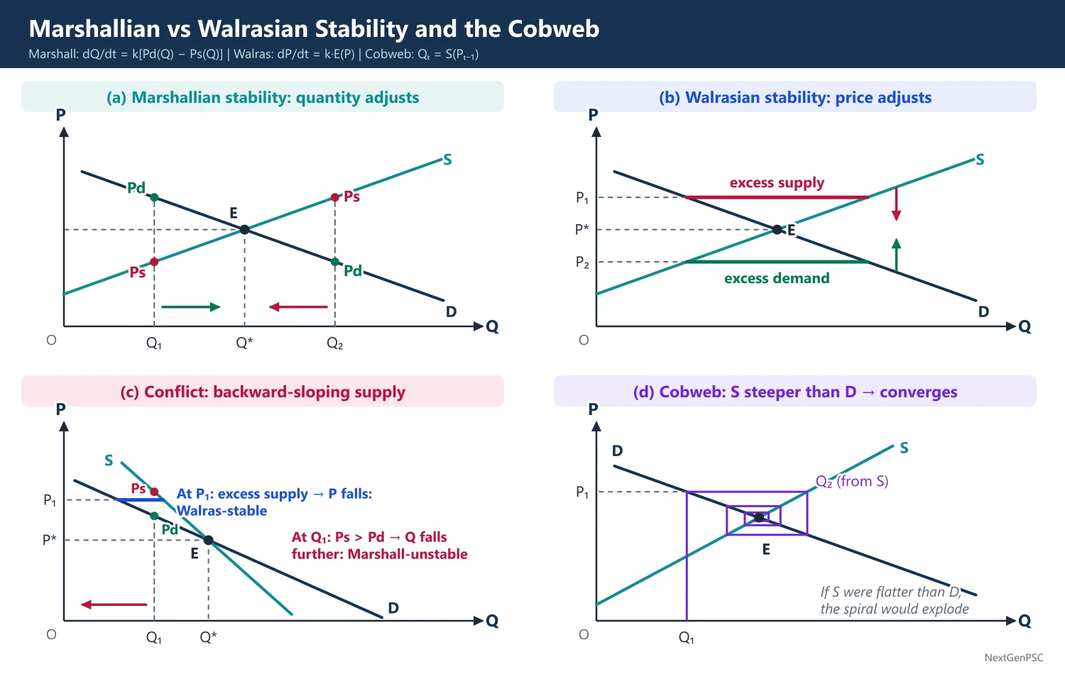
Marshall (1890) studied one market at a time (partial equilibrium) with quantity adjustment: output expands when demand price exceeds supply price. Walras (1874) studied all markets together (general equilibrium) with price adjustment: price rises when there is excess demand. The two stability conditions agree for normal curves but give opposite verdicts when both curves slope the same way.
In simple words
Price determination asks how the price of a good is fixed by buyers and sellers.
Marshall looked at one market, like rice, keeping everything else fixed; Walras looked at all markets together, because the price of rice affects wheat, wages and transport.
Think of Marshall as zooming in with a camera and Walras as taking a wide-angle photo of the whole city.
UPSC asks you to compare the two and to explain their stability conditions with diagrams.
1. The problem and two traditions
Price determination: how the price of a good and the quantity traded are fixed by the interaction of demand and supply.
Alfred Marshall: Principles of Economics (1890) built the partial equilibrium approach: study one market at a time, holding other prices, incomes and tastes constant (ceteris paribus).
Léon Walras: Éléments d'économie politique pure (1874) built the general equilibrium approach: all markets are interdependent and all prices are determined simultaneously.
Scissors analogy: Marshall argued that asking whether utility (demand) or cost of production (supply) governs value is like asking which blade of a pair of scissors cuts the paper; both do.
Time element: Marshall's key innovation: market period (supply fixed, demand dominates), short period (output varies with given plant), long period (plant and number of firms adjust, cost dominates) and secular period.
2. Marshallian approach step by step
Assumptions: perfect competition, one market studied in isolation, other things equal, cardinal utility with a constant marginal utility of money, sellers adjust quantity.
Demand price Pd(Q): the maximum price buyers will pay for quantity Q, read off the demand curve.
Supply price Ps(Q): the minimum price sellers need in order to supply Q, read off the supply curve.
Quantity adjustment rule: if Pd(Q) exceeds Ps(Q), producers earn more than they need and expand output; if Pd(Q) is below Ps(Q) they contract: dQ/dt = k[Pd(Q) − Ps(Q)], k > 0.
Equilibrium: the quantity Q* at which Pd(Q*) = Ps(Q*).
Marshallian stability condition: to the left of Q* demand price exceeds supply price and to the right supply price exceeds demand price; mathematically Pd′(Q*) is less than Ps′(Q*), i.e. the slope of the inverse demand curve is less than that of the inverse supply curve.
Why quantity adjusts: Marshall had in mind producers changing output over time, especially in the long period, where decreasing-cost industries (external economies) can have a downward-sloping supply curve.
3. Walrasian approach step by step
Assumptions: perfect competition in every market, flexible prices, an auctioneer who calls out prices (tâtonnement, 'groping'), no trade at disequilibrium prices.
Excess demand: E(P) = D(P) − S(P), the gap between quantity demanded and quantity supplied at price P.
Price adjustment rule: price rises when there is excess demand and falls when there is excess supply: dP/dt = k·E(P), k > 0.
Equilibrium: the price P* at which E(P*) = 0.
Walrasian stability condition: excess demand falls as price rises, dE/dP less than 0, i.e. D′(P) less than S′(P): above P* there is excess supply and below P* excess demand.
General equilibrium form: with n markets the system is Eᵢ(p₁, ..., pₙ) = 0 for every i, solved simultaneously (see the next topic).
4. When the two stability conditions conflict
Normal curves: with a downward-sloping demand curve and an upward-sloping supply curve, equilibrium is stable in both senses.
Backward-sloping supply, steeper than demand: (e.g. labour supply at high wages, or a decreasing-cost industry) equilibrium is Walras-stable but Marshall-unstable.
Backward-sloping supply, flatter than demand: equilibrium is Marshall-stable but Walras-unstable.
Upward-sloping demand (Giffen case) with normal supply: again one criterion says stable and the other unstable; it is Walras-stable if the supply curve is flatter than the demand curve and Marshall-stable if it is steeper.
Reason: Walras compares quantities at a given price (the horizontal gap); Marshall compares prices at a given quantity (the vertical gap); the slopes enter as reciprocals, so whenever both curves slope the same way exactly one criterion is satisfied.
Later work: J.R. Hicks in Value and Capital (1939) extended Walrasian stability to many markets; P.A. Samuelson in Foundations of Economic Analysis (1947) showed that stability is a dynamic question that depends on the assumed adjustment process.
5. Dynamic case: the cobweb model
Origin: the cobweb theorem was named by Kaldor (1934) and set out by Mordecai Ezekiel (1938) for farm markets where output is planned on last season's price.
Equations: Dₜ = a − bPₜ; Sₜ = c + dPₜ₋₁; market clearing Dₜ = Sₜ gives Pₜ = (a − c)/b − (d/b)Pₜ₋₁.
Convergence condition: the price path converges if d/b is less than 1, i.e. supply responds less than demand; with P on the vertical axis the supply curve is steeper than the demand curve; d = b gives a perpetual cycle and d > b an explosive one.
Indian example: boom-and-bust cycles in onion, tomato and potato prices, where a high price this season induces heavy sowing and a glut next season; MSP, buffer stocks and price stabilisation funds try to break the cycle.
6. Diagrams to draw
Marshallian stability: Q on the horizontal axis and P on the vertical; draw D and S crossing at E; at Q1 left of Q* mark demand price A above supply price B with an arrow pointing right; at Q2 right of Q* mark supply price above demand price with an arrow pointing left.
Walrasian stability: same axes; at a price P1 above P* show the horizontal gap between D and S labelled 'excess supply' with a downward arrow; at P2 below P* label 'excess demand' with an upward arrow.
Conflict case: draw a downward-sloping demand curve and a backward-sloping supply curve steeper than demand; show that above P* there is excess supply (price falls back: Walras-stable) while at a quantity below Q* supply price exceeds demand price (output shrinks further: Marshall-unstable).
Cobweb: draw D and a steeper S; start from a low output Q1, read the price P1 off D, then output Q2 off S at P1, and so on; the spiral closes in on E (convergent); redraw with a flatter S for the explosive case.
7. Comparing the approaches and debates
Partial versus general: Marshall is simple and practical for a single market with small spillovers; Walras captures interdependence (a fall in the price of tea affects coffee, sugar and wages).
Criticism of Marshall: ceteris paribus fails when the market is large (e.g. labour or energy); a constant marginal utility of money ignores income effects.
Criticism of Walras: the auctioneer and no trade before equilibrium are unrealistic; counting equations and unknowns does not prove that a solution exists (proved later by Arrow and Debreu, 1954).
Modern practice: partial equilibrium is used for single markets and computable general equilibrium (CGE) models for economy-wide policies such as trade agreements or tax reforms.
Indian applications: MSP and procurement of wheat and rice (a partial-equilibrium price floor); the GST, which changed relative prices across all sectors at once (a general-equilibrium question).
8. Using it in the exam
10 marks: define both approaches, state the two stability conditions and draw one small diagram.
15 marks: both adjustment rules with equations, the conflict case with a diagram, and a conclusion on when each applies.
20 marks: add the time element, cobweb dynamics with its convergence condition, criticisms and an Indian farm-price example.
Keywords: partial equilibrium, ceteris paribus, demand price, supply price, excess demand, tâtonnement, stability condition, cobweb.
Quotation: Marshall's scissors analogy, paraphrased: neither utility nor cost alone determines value, just as neither blade alone cuts the paper.
| Basis | Marshall (1890) | Walras (1874) |
|---|---|---|
| Scope | Partial equilibrium: one market | General equilibrium: all markets |
| Adjusting variable | Quantity | Price |
| Signal | Demand price minus supply price | Excess demand |
| Stability condition | Pd′(Q) less than Ps′(Q) | D′(P) less than S′(P) |
| Time | Market, short, long and secular periods | Timeless, auctioneer process |
| Best suited to | Long-period output decisions, single industries | Interdependent markets, economy-wide policy |
Mains points
- Always state both adjustment rules with equations: dQ/dt = k[Pd(Q) − Ps(Q)] for Marshall and dP/dt = k·E(P) for Walras.
- The favourite question is the conflict case: show with a backward-sloping supply curve that an equilibrium can be stable in one sense and unstable in the other.
- Link Marshall's quantity adjustment to the long period and decreasing-cost industries, and Walras' price adjustment to markets with flexible prices.
- Add the cobweb model for dynamics, with its exact convergence condition, and an Indian vegetable-price example.
- Do not confuse partial equilibrium with the short run; partial refers to the number of markets, not the time period.
- Conclude that the approaches are complementary: Marshall for single-market analysis, Walras and CGE models for interdependence.
Did you know?
- Memory trick: 'Marshall Moves Quantity, Walras Wiggles Price' (MQ-WP).
- Walras modelled tâtonnement on organised markets such as the Paris Bourse, where brokers call out prices; the term 'Walrasian auctioneer' was added by later economists.
General Equilibrium: Existence, Stability and Walras' Law
General equilibrium is a price vector at which all markets clear together. Walras' Law says the value of aggregate excess demand is always zero, so if n − 1 markets clear the nth does too. Existence was proved by Arrow and Debreu (1954) using fixed-point theorems under convexity; uniqueness and stability need extra conditions such as gross substitutability.
In simple words
General equilibrium means every market in the economy, from food to labour to steel, balances at the same time.
It is like a large group of friends splitting a restaurant bill: if everyone except one has paid the right share, the last person's share is automatically fixed; that is Walras' Law.
Economists asked whether such balancing prices exist, whether there is only one set, and whether markets actually reach them.
UPSC asks you to state Walras' Law, explain existence and stability, and draw the Edgeworth box.
1. Concepts and definitions
General equilibrium: a set of prices at which every market in the economy clears at the same time, given consumers' preferences and endowments and firms' technologies (Walras, 1874).
Excess demand function: Eᵢ(p) = Dᵢ(p) − Sᵢ(p) for each good i, where p is the vector of all prices.
Homogeneity: excess demands are homogeneous of degree zero in prices: doubling all prices (and hence money incomes) leaves real choices unchanged, so only relative prices matter.
Numéraire: one good whose price is set equal to 1; the other n − 1 prices are measured in terms of it.
Tâtonnement: Walras' 'groping' process in which prices are adjusted according to excess demand and no trade takes place until equilibrium is found.
2. Walras' Law
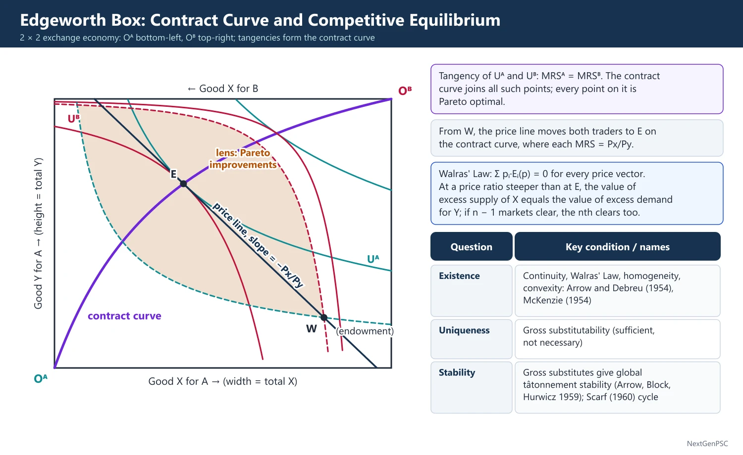
Statement: the value of aggregate excess demand is identically zero: Σ pᵢ·Eᵢ(p) = 0 for every price vector, not only at equilibrium.
Derivation: each household's budget constraint says that the value of what it buys equals the value of what it sells (endowment plus profit income); summing over all households gives the law.
Implication 1: if n − 1 markets are in equilibrium, the nth market must also be in equilibrium.
Implication 2: only n − 1 equations are independent, matching the n − 1 relative prices to be determined.
Implication 3: excess demand (in value) in one market must be matched by excess supply somewhere else, so a general glut of all goods is impossible in a barter economy; this links Walras' Law with Say's Law.
Money and Walras' Law: Don Patinkin, in Money, Interest and Prices (1956), argued that the classical dichotomy between the real and monetary sectors is inconsistent once money enters Walras' Law, and resolved it with the real balance effect (debated).
Keynesian challenge: Robert Clower (1965) argued that unemployed workers cannot turn their notional demand for goods into effective demand, so Walras' Law holds for notional demands but not for effective demands (the dual-decision hypothesis).
3. Existence of equilibrium
Counting equations: Walras argued that n − 1 independent equations in n − 1 unknowns give a solution; this is neither necessary nor sufficient, since solutions may involve negative prices, be multiple or not exist.
Rigorous proofs: Abraham Wald (1930s) for special cases; Kenneth Arrow and Gerard Debreu (Econometrica, 1954) and Lionel McKenzie (1954) for the general competitive economy, using fixed-point theorems (Brouwer, Kakutani).
Conditions for existence: continuous excess demand functions, Walras' Law, homogeneity of degree zero, convex preferences and convex production sets (no increasing returns), and every household owning something of value.
Why convexity matters: with increasing returns or non-convex preferences demand or supply can jump, and an equilibrium price vector may fail to exist.
Uniqueness: not guaranteed in general; it holds if all goods are gross substitutes, i.e. a rise in pⱼ raises the excess demand for every other good i (∂Eᵢ/∂pⱼ > 0 for i ≠ j).
4. Stability of equilibrium
Question: if prices start away from equilibrium, does the adjustment process bring them back?
Hicks: in Value and Capital (1939) Hicks defined perfect stability: a rise in a price must create excess supply in that market whether other prices stay fixed or adjust; this is a condition on the signs of the principal minors of the matrix of excess demand derivatives.
Samuelson: in 1941 and in Foundations of Economic Analysis (1947) Samuelson treated stability dynamically, dpᵢ/dt = kᵢ·Eᵢ(p), and showed that Hicksian conditions are in general neither necessary nor sufficient for dynamic stability; his correspondence principle links stability to comparative statics.
Arrow, Block and Hurwicz (1959): tâtonnement is globally stable if all goods are gross substitutes.
Herbert Scarf (1960): built a three-good example in which tâtonnement cycles for ever, so stability is not a general property.
Sonnenschein-Mantel-Debreu results (1972–74): aggregate excess demand functions need satisfy only continuity, homogeneity and Walras' Law, so almost any behaviour, including instability and multiple equilibria, is possible.
Non-tâtonnement processes: models in which trade takes place at disequilibrium prices (Edgeworth's recontracting; Hahn and Negishi, 1962) are closer to real markets.
5. The 2 × 2 exchange and production model
Pure exchange: two consumers A and B, two goods X and Y, fixed endowments, shown in the Edgeworth box (after F.Y. Edgeworth, 1881; also called the Edgeworth-Bowley box).
Contract curve: the locus of tangencies of A's and B's indifference curves, where MRSᴬ = MRSᴮ; every point on it is Pareto efficient.
Competitive equilibrium: a price line through the endowment point tangent to both consumers' indifference curves at the same point; there MRSᴬ = MRSᴮ = Px/Py and the two offer curves intersect.
With production: two factors (L, K) are allocated between X and Y; efficiency needs MRTSˣ = MRTSʸ (production contract curve), which maps into the production possibility frontier; overall equilibrium needs MRS = MRT = Px/Py.
6. Diagrams to draw
Edgeworth box: a rectangle with A's origin at the bottom-left and B's at the top-right; width = total X, height = total Y; draw A's indifference curves convex to OA and B's convex to OB; join the tangency points to form the contract curve from OA to OB.
Equilibrium in the box: mark the endowment point W off the contract curve; draw the price line through W tangent to one indifference curve of each consumer at the same point E on the contract curve; label its slope −Px/Py.
Walras' Law in a two-good economy: at a price ratio steeper than equilibrium, show A and B together demanding less X than available and more Y than available, with equal values of excess supply and excess demand.
7. Applications and debates
Interdependence in practice: a crude oil price shock raises transport costs, food prices, the fertiliser subsidy bill and India's current account deficit at once; a general equilibrium view captures these links.
CGE models: computable general equilibrium models are used worldwide to study tariff cuts, trade agreements and tax reforms such as India's GST.
Criticism: the Arrow-Debreu world has no money, no sequence of markets over time and no role for institutions; Frank Hahn argued that money has no essential role in it (debated).
Defence: it provides the benchmark against which market failures (externalities, public goods, monopoly) are defined and underpins the fundamental theorems of welfare economics.
8. Using it in the exam
10 marks: state Walras' Law, derive it from budget constraints and give its implication for n − 1 markets.
15 marks: existence conditions with names (Arrow-Debreu, 1954) and an Edgeworth box diagram.
20 marks: Walras' Law, existence, uniqueness (gross substitutes) and stability (Hicks, Samuelson, Scarf), with criticism (Clower, Sonnenschein-Mantel-Debreu).
Keywords: excess demand, homogeneity of degree zero, numéraire, Walras' Law, fixed-point theorem, gross substitutes, tâtonnement.
Definition to quote: Walras' Law: the sum of the values of excess demands over all markets is zero, so if n − 1 markets clear, the nth must also clear.
| Question | Key condition | Main contributors |
|---|---|---|
| Existence | Continuity, Walras' Law, homogeneity, convexity | Wald; Arrow and Debreu (1954); McKenzie (1954) |
| Uniqueness | Gross substitutability (sufficient, not necessary) | Arrow, Hurwicz and others |
| Stability | Gross substitutes give global tâtonnement stability; not general | Hicks (1939); Samuelson (1947); Arrow, Block and Hurwicz (1959); Scarf (1960) |
| Limits | Aggregate excess demand can take almost any shape | Sonnenschein, Mantel, Debreu (1972–74) |
Mains points
- Derive Walras' Law from summed budget constraints in two or three lines; examiners reward the derivation, not just the statement.
- Distinguish clearly between existence, uniqueness and stability; many answers mix them up.
- Explain why counting equations is not enough and name the fixed-point proof by Arrow and Debreu (1954).
- Use the Edgeworth box to show competitive equilibrium on the contract curve and to link to Pareto efficiency.
- Add the Keynesian critique (Clower's dual decision) and the Patinkin debate on money for a critical answer.
- Give one real example of interdependence, such as an oil shock spreading through Indian prices and the current account.
Did you know?
- Both Arrow (1972) and Debreu (1983) received the Nobel Prize in Economics, partly for their work on general equilibrium.
Ricardian Theory of Distribution
Ricardo (1817) divided output among landlords (rent), capitalists (profit) and workers (wages). Rent is a differential surplus on better land, wages stay at subsistence, and profit is the residual. As accumulation pushes cultivation to worse land, rent rises, the rate of profit falls and the economy approaches a stationary state.
In simple words
Ricardo asked how a country's harvest is shared among landlords, business owners and workers.
Imagine a village where the best fields are farmed first; when more food is needed, poorer fields are used, and owners of the good fields can charge more rent.
Workers get just enough to live, so as rent rises, the business owners' profit shrinks and growth slows down.
UPSC asks you to explain differential rent, the falling rate of profit and the stationary state, often comparing Ricardo with Kaldor.
1. Setting and concepts
Source: David Ricardo, On the Principles of Political Economy and Taxation (1817); in the preface he called determining the laws that regulate distribution among landlords, capitalists and labourers 'the principal problem in Political Economy'.
Three classes and three incomes: landlords receive rent, capitalists receive profit and workers receive wages.
Macro view: Ricardo studied the shares of total output going to each class and how they change as the economy grows, not the pricing of individual factors.
Rent (Ricardo's definition): 'that portion of the produce of the earth which is paid to the landlord for the use of the original and indestructible powers of the soil'.
Natural wage: the wage that allows workers to subsist and perpetuate their numbers without increase or decrease; market wages move around it through Malthusian population changes.
Profit: the residual left to the capitalist after rent and wages; the rate of profit drives accumulation.
2. Assumptions
One good: corn is both output and wage good (the 'corn model', as reconstructed by Kaldor in 1956 and by Sraffa).
Land: fixed in supply and of different fertility; diminishing returns operate at the extensive margin (worse land) and the intensive margin (more doses on the same land).
Wages and capital: wages stay at subsistence in the long run (Malthusian population principle); capital is the wage fund advanced to workers.
Market and technology: perfect competition, so the rate of profit is equal in all uses; closed economy; no technical progress.
3. The model step by step
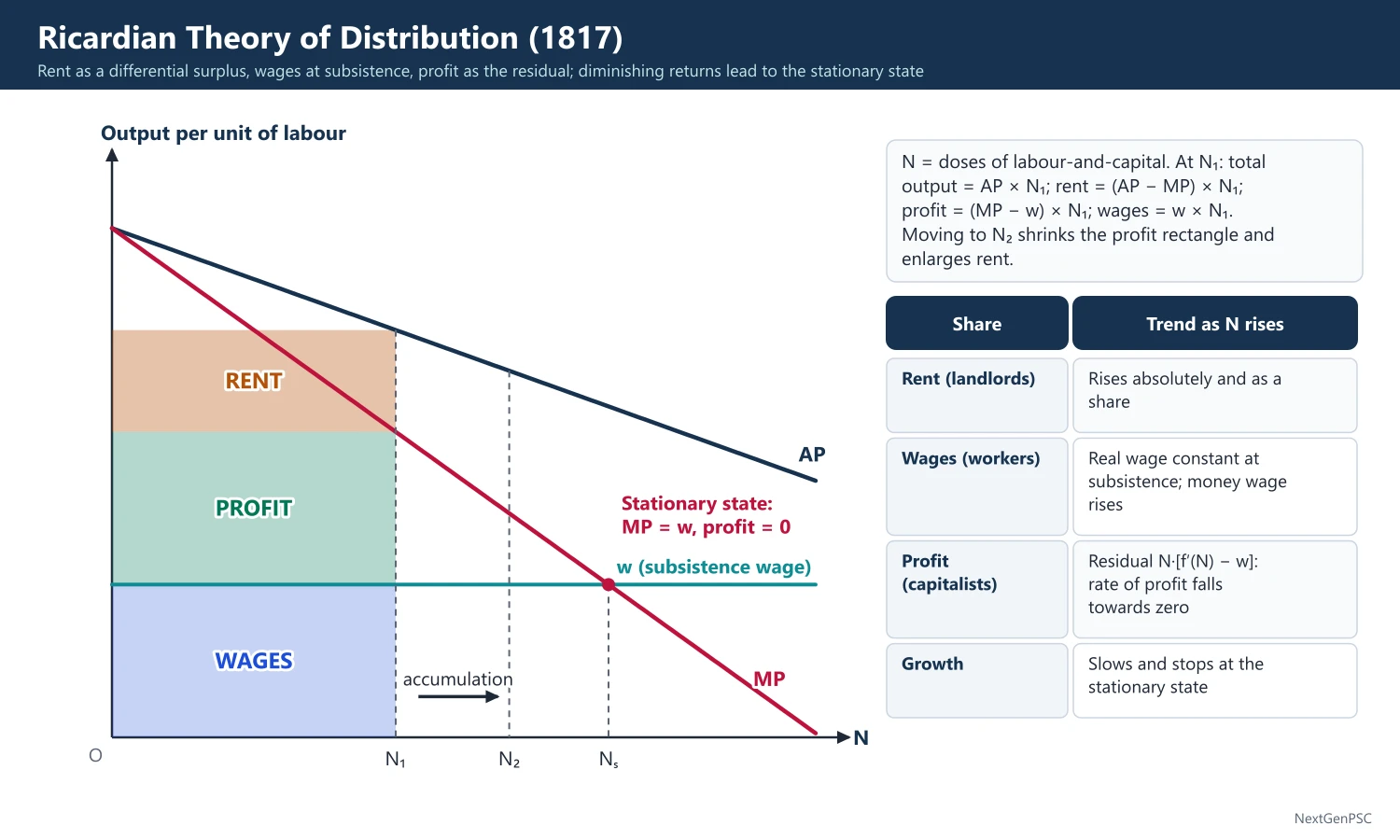
Output: Y = f(N), where N is the number of workers (doses of labour-and-capital), with f′ > 0 and f″ less than 0 (diminishing returns).
Rent: the marginal land pays no rent; rent on any better plot equals its surplus over the marginal plot; in aggregate R = f(N) − N·f′(N), i.e. (average product − marginal product) × N.
Wages: W = w·N, where w is the subsistence wage per worker.
Profit: Π = N·[f′(N) − w], the marginal product net of the wage on every unit.
Rate of profit: r = [f′(N) − w]/w, since capital is the wage fund w·N.
Price-determined rent: the price of corn is set by the cost on the marginal (no-rent) land; in Ricardo's words, corn is not high because a rent is paid, but a rent is paid because corn is high.
4. Dynamics: towards the stationary state
Accumulation: positive profits → capitalists accumulate → demand for labour rises → market wage rises above subsistence → population grows.
Extension of cultivation: more workers must be fed, so worse land is brought in and f′(N) falls.
Shares change: rent per acre and the rent share rise; the money wage rises because corn becomes dearer, but the real wage stays at subsistence; the rate of profit falls.
Stationary state: when f′(N) falls to w, profit falls to zero (or to the minimum needed to compensate risk), accumulation stops and growth ends.
Landlords gain: the only class whose income rises without effort; Ricardo concluded that the landlord's interest is opposed to that of the rest of society.
Policy, the Corn Laws: Ricardo argued that free import of corn would halt the move to worse land, lower rent and raise the rate of profit; the Corn Laws were repealed in 1846, after his death in 1823.
5. Diagram to draw
Axes: horizontal axis: labour (doses of labour-and-capital) N; vertical axis: output per unit of labour.
Curves: a downward-sloping average product (AP) curve and a steeper marginal product (MP) curve below it; a horizontal line at the subsistence wage w.
Shares at employment N1: total output = AP × N1 (rectangle under AP); rent = area between AP and MP up to N1; profit = rectangle between MP and the wage line; wages = rectangle below w.
Growth: move N to the right, to N2: the profit rectangle shrinks and the rent area grows; at Ns, where MP = w, the profit rectangle vanishes: the stationary state.
6. Criticisms and debates
Technical progress ignored: improvements in agriculture postponed diminishing returns indefinitely; the stationary state never arrived in the industrial countries.
Population theory: fertility fell as incomes rose, contrary to the Malthusian link between wages and population.
Theory of rent: Marx added absolute rent; scarcity rent exists even on land of uniform quality; rent also arises in non-farm uses such as urban land and minerals.
Value problem: Ricardo searched for an invariable measure of value; Piero Sraffa's Production of Commodities by Means of Commodities (1960) revived the classical approach with the standard commodity.
Marginal productivity theory: the neo-classical approach (J.B. Clark, Wicksteed) later explained each factor's income by its marginal product, a micro theory; Ricardo's theory is macro and class-based.
Relevance today: debated; Thomas Piketty's Capital in the Twenty-First Century (2013) revived the classical focus on long-run shares, and land and housing rents absorb a large share of income in many growing cities.
7. Indian applications
Differential rent in India: irrigated, fertile land in Punjab or the Godavari delta commands higher rents and sale values than rain-fed land; crop-share rents of half the produce were common before land reforms.
Zamindari and rent: colonial land systems transferred the agrarian surplus to intermediaries rather than to productive investment, which post-1947 land reforms sought to end.
Diminishing returns and fragmentation: the average operational holding fell from 2.28 hectares in 1970–71 to 1.08 hectares in 2015–16 (Agriculture Census), pressing on returns per worker.
Technical change: high-yielding varieties, irrigation and fertiliser in the 1960s and 1970s shifted the MP curve upward, the opposite of Ricardo's prediction.
8. Using it in the exam
10 marks: three classes, differential rent, profit as residual, stationary state.
15 marks: equations for R, W and Π, the AP-MP diagram and the falling rate of profit.
20 marks: add assumptions, the Corn Laws, criticism (technical progress, Malthus, Sraffa) and Kaldor's comparison with other theories.
Keywords: differential rent, extensive and intensive margins, subsistence wage, wage fund, falling rate of profit, stationary state.
Quotation: Ricardo (1817): corn is not high because a rent is paid, but a rent is paid because corn is high.
| Income | How determined | Trend with accumulation |
|---|---|---|
| Rent (landlords) | Surplus of intramarginal over marginal land: f(N) − N·f′(N) | Rises absolutely and as a share |
| Wages (workers) | Subsistence wage × workers: w·N | Real wage constant; money wage rises |
| Profit (capitalists) | Residual: N·[f′(N) − w] | Rate of profit falls towards zero |
| Growth | Driven by the rate of profit | Slows and stops at the stationary state |
Mains points
- Present the theory as a macro, class-based theory and contrast it with marginal productivity (micro) theory.
- Give the three equations (rent, wages, profit) and the AP-MP diagram; this is the standard reconstruction from Kaldor (1956).
- Explain why rent is price-determined, not price-determining, with Ricardo's corn quotation.
- Trace the chain from accumulation to the stationary state step by step; examiners look for the falling rate of profit.
- Criticise with technical progress, the failure of Malthusian population theory and the neglect of non-agricultural rent.
- Bring in an Indian angle: differential rent on irrigated land, land reforms, and the Green Revolution as a counter to diminishing returns.
Did you know?
- Ricardo made a fortune as a stockbroker and government bond dealer before writing economics, and later sat in the British Parliament.
Kaldor and Kalecki: Macro Theories of Distribution
Kaldor (1955–56) explained the profit share by investment and saving propensities at full employment: P/Y = [1/(sp − sw)]·(I/Y) − sw/(sp − sw), stable only if sp > sw. Kalecki explained the wage share by the degree of monopoly (mark-up over prime cost) and showed that capitalists' spending determines profits. Both reject marginal productivity as the explanation of shares.
In simple words
These theories explain what share of national income goes to wages and what share to profits.
Kaldor said that when businesses invest more, prices rise faster than wages and profits grow; Kalecki said firms add a mark-up to costs, like a shop adding a fixed margin to the wholesale price, and stronger firms add more.
This matters for inequality, demand and policy on competition and wages.
UPSC asks you to derive Kaldor's equation and explain Kalecki's degree of monopoly.
1. Macro theories of distribution
Question: what determines the shares of wages and profits in national income?
Neo-classical answer: marginal productivity: each factor earns its marginal product (J.B. Clark, The Distribution of Wealth, 1899); with a Cobb-Douglas production function the shares are constant.
Post-Keynesian answer: shares are determined by aggregate demand, saving behaviour and market power; the two main versions are Nicholas Kaldor's and Michał Kalecki's.
Kaldor's survey: in 'Alternative Theories of Distribution' (Review of Economic Studies, 1955–56) Kaldor compared the Ricardian, Marxian, neo-classical and Keynesian theories and built his own Keynesian theory.
2. Kaldor's model: assumptions
Full employment: total output Y is given in the long run.
Two classes: workers save a fraction sw of wages W and capitalists save a fraction sp of profits P, with sp > sw.
Exogenous investment: I is set by the growth rate and technical progress, independently of saving; saving adjusts to investment.
Flexible prices: prices are flexible relative to money wages, so profit margins adjust.
3. Kaldor's model: equations and mechanism
Identities: Y = W + P and I = S.
Saving: S = sw·W + sp·P = sw·Y + (sp − sw)·P.
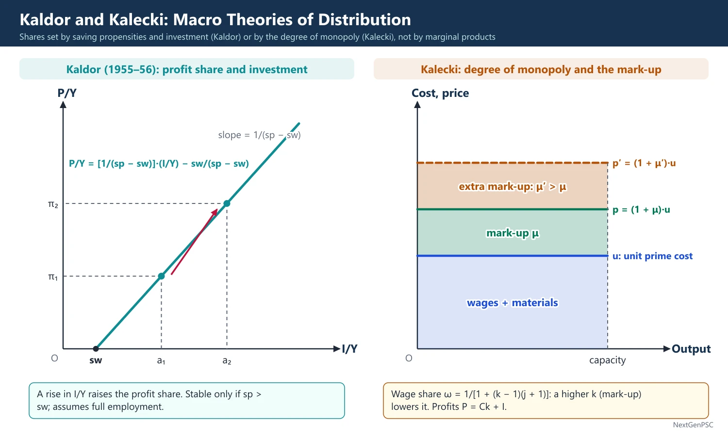
Profit share: setting I = S and dividing by Y gives P/Y = [1/(sp − sw)]·(I/Y) − sw/(sp − sw).
Special case sw = 0: P/Y = (1/sp)·(I/Y) and P = I/sp; profits are determined by investment and capitalists' saving propensity.
Rate of profit: with sw = 0, P/K = (1/sp)·(I/K) = g/sp, where g is the growth rate of the capital stock (the 'Cambridge equation').
Mechanism: a rise in I/Y creates excess demand at full employment; prices rise faster than money wages; the profit share rises; since sp > sw, total saving rises until S equals the higher I.
Coefficient of sensitivity: 1/(sp − sw) shows how strongly the profit share responds to a change in the investment ratio; the smaller the gap between sp and sw, the larger the response.
Widow's cruse: Kaldor used Keynes' image from the Treatise on Money (1930): what capitalists spend on investment or consumption returns to them as profit, however much they spend.
4. Conditions and limits of Kaldor's model
Stability condition: sp > sw; if sw ≥ sp, a rise in investment would not raise saving enough and the system would be unstable.
Wage floor: the real wage cannot fall below a subsistence minimum, so W/Y has a lower bound.
Profit floor: the profit share cannot fall below the minimum set by the degree of monopoly or the risk premium.
Investment range: the investment ratio must lie between sw and sp (sw ≤ I/Y ≤ sp) for the profit share to lie between 0 and 1.
Pasinetti (1962): pointed out that workers who save must own capital and earn profit on it; correcting this, he showed that in long-run steady growth r = g/sc (sc = capitalists' saving propensity), independent of workers' saving: the Pasinetti theorem.
Samuelson and Modigliani (1966): replied with the 'anti-Pasinetti' (dual) theorem: if workers save enough, the capitalist class disappears and the capital-output ratio is governed by sw alone (debated).
5. Kalecki's theory: degree of monopoly
Source: Michał Kalecki, Essays in the Theory of Economic Fluctuations (1939) and Theory of Economic Dynamics (1954).
Pricing: manufacturing firms with excess capacity set prices as a mark-up on unit prime cost (wages plus materials): p = (1 + μ)·u, where u is unit prime cost and μ the mark-up.
Degree of monopoly k: the ratio of aggregate proceeds to aggregate prime costs; a higher k means a higher mark-up.
Wage share formula: ω = W/Y = 1/[1 + (k − 1)(j + 1)], where j is the ratio of materials cost to the wage bill; the wage share falls when k or j rises.
Determinants of k: industrial concentration, advertising and sales promotion replacing price competition, the level of overheads relative to prime costs, and the strength of trade unions (strong unions restrain mark-ups).
Profit equation: in a closed economy without government and with workers who do not save, P = Ck + I (capitalists' consumption plus investment); more generally P = I + (G − T) + (X − M) + Ck − Sw.
Causation: capitalists can decide what they spend but not what they earn, so their spending determines profits; the saying 'workers spend what they earn, capitalists earn what they spend' is usually associated with Kalecki.
6. Diagrams to draw
Kaldor: horizontal axis I/Y, vertical axis P/Y; draw the upward line P/Y = [1/(sp − sw)]·(I/Y) − sw/(sp − sw), with slope 1/(sp − sw) and horizontal intercept at I/Y = sw; show a rise in I/Y from a1 to a2 raising P/Y from π1 to π2.
Kalecki: horizontal axis output, vertical axis cost and price; draw a flat unit prime cost line u up to capacity and a price line p = (1 + μ)·u above it; the gap is the mark-up; show that a rise in μ widens the profit band and lowers the wage share at the same output.
7. Comparison, criticism and Indian relevance
Kaldor versus Kalecki: Kaldor assumes full employment and flexible prices, so distribution adjusts to investment; Kalecki assumes excess capacity and mark-up pricing, so output adjusts to demand and distribution depends on market power.
Criticism of Kaldor: full employment is unrealistic for most economies; saving propensities are taken as given; it is a long-run theory often tested on short-run data (debated).
Criticism of Kalecki: the degree of monopoly is hard to measure, and Kaldor called the theory close to a tautology, since k is defined from the outcome itself.
Indian relevance: studies using Annual Survey of Industries data report a long-run fall in the share of wages in the gross value added of organised manufacturing, consistent with rising mark-ups and capital intensity; concentration in sectors such as telecom and aviation raises Kaleckian questions about market power.
Fiscal link: Kalecki's profit equation implies that, other things equal, a larger government deficit or trade surplus raises aggregate profits and a fiscal squeeze lowers them.
8. Using it in the exam
10 marks: Kaldor's equation P/Y = [1/(sp − sw)]·(I/Y) − sw/(sp − sw) with the stability condition sp > sw.
15 marks: Kalecki's degree of monopoly, the wage-share formula and the determinants of k.
20 marks: both models, Pasinetti's correction, a comparison table with Ricardo and marginal productivity, criticism and an Indian example.
Keywords: saving propensities, investment ratio, widow's cruse, Cambridge equation, Pasinetti theorem, mark-up, degree of monopoly, profit equation.
Definition to quote: Kalecki's degree of monopoly is the ratio of aggregate proceeds to aggregate prime costs.
| Basis | Ricardo (1817) | Marginal productivity (Clark, 1899) | Kaldor (1955–56) | Kalecki (1939, 1954) |
|---|---|---|---|---|
| Level | Macro, class-based | Micro, factor-based | Macro | Macro with micro pricing |
| Key determinant | Diminishing returns on land | Marginal products of factors | Investment ratio and saving propensities | Degree of monopoly (mark-up) |
| Employment assumption | Subsistence wages, growing labour | Full employment | Full employment | Excess capacity, unemployment |
| Main result | Rent share rises, profit rate falls | Factor shares equal output elasticities | Higher I/Y raises profit share | Higher k lowers wage share; spending determines profits |
Mains points
- Derive Kaldor's equation from Y = W + P and I = S in four lines; state sp > sw as the stability condition and the limits (wage floor, profit floor).
- Explain the mechanism in words: investment → excess demand → prices rise relative to wages → profit share rises → saving catches up.
- For Kalecki, give the mark-up rule, the wage-share formula and the four determinants of the degree of monopoly.
- Add Pasinetti's theorem (r = g/sc) for a high-scoring answer on Kaldor.
- Contrast both with marginal productivity theory and Ricardo in a table.
- Use an Indian example: the falling wage share in organised manufacturing (ASI) or concentration in telecom and aviation.
Did you know?
- Kalecki published the core of the effective demand idea in Polish in 1933, before Keynes' General Theory (1936), which is why some call him a co-discoverer of the theory.
Consumer, Production and Cost Theory: Foundations
Consumer theory derives demand from utility maximisation: equilibrium where MRS = Px/Py; a price change splits into substitution and income effects (Slutsky equation), giving Marshallian (uncompensated) and Hicksian (compensated) demand. Producer theory uses production functions such as Cobb-Douglas and CES, Euler's theorem for factor shares, and cost curves; a competitive firm's supply curve is its MC above minimum AVC.
In simple words
These are the building blocks behind demand and supply curves: how a buyer chooses, and how a firm produces at least cost.
When the price of tea falls you buy more partly because it is cheaper than coffee (substitution effect) and partly because you feel richer (income effect).
Firms combine labour and machines like a cook combines ingredients, and their cost curves give the supply curve.
UPSC asks for the Slutsky equation, compensated demand, Cobb-Douglas properties, Euler's theorem and deriving supply from costs.
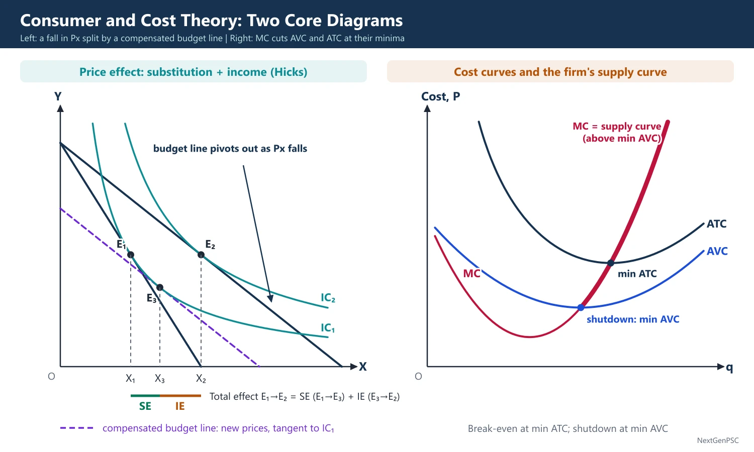
1. Consumer theory: utility and indifference curves
Cardinal utility (Marshall): utility is measurable; the consumer is in equilibrium when MUx/Px = MUy/Py = marginal utility of money, based on the law of diminishing marginal utility.
Ordinal utility: Hicks and Allen (1934) and Hicks (Value and Capital, 1939): the consumer only ranks bundles; an indifference curve joins bundles giving equal satisfaction; it slopes down, is convex to the origin (diminishing MRS) and indifference curves do not intersect.
Marginal rate of substitution: MRSxy = −dY/dX along an indifference curve = MUx/MUy.
Budget line: Px·X + Py·Y = M, with slope −Px/Py.
Equilibrium: MRSxy = Px/Py at a tangency, with convex indifference curves as the second-order condition.
Revealed preference: Paul Samuelson (1938, 1948) derived demand from observed choices; the weak axiom says that if bundle A is chosen when B was affordable, B is never chosen when A is affordable.
2. Income and substitution effects and the Slutsky equation
Price effect: the total change in quantity demanded = substitution effect + income effect.
Hicksian decomposition: income is adjusted so the consumer stays on the original indifference curve; the substitution effect is always opposite in sign to the price change.
Slutsky decomposition (1915): income is adjusted so that the original bundle remains just affordable (cost-difference compensation).
Slutsky equation: ∂x/∂Px = ∂xʰ/∂Px − x·(∂x/∂M), where the first term (substitution) is negative and the second is the income effect.
Normal, inferior and Giffen goods: for a normal good both effects reinforce; for an inferior good the income effect works against the substitution effect but demand still slopes down if the substitution effect dominates; a Giffen good is an inferior good whose income effect outweighs the substitution effect, so demand slopes upward (evidence: Jensen and Miller, 2008, rice among poor households in Hunan, China).
3. Marshallian versus Hicksian demand
Marshallian (uncompensated) demand x(P, M): from utility maximisation subject to the budget; it includes both effects.
Hicksian (compensated) demand xʰ(P, U): from expenditure minimisation for a given utility; it shows only the substitution effect and always slopes downward.
Relation: the two curves pass through the original point; the Hicksian curve is steeper (less elastic) than the Marshallian for a normal good and flatter for an inferior good.
Duality: the indirect utility function V(P, M) and the expenditure function E(P, U); Roy's identity x = −(∂V/∂P)/(∂V/∂M); Shephard's lemma xʰ = ∂E/∂P.
Welfare measures: Hicks' compensating and equivalent variations are measured with Hicksian demand; Marshallian consumer surplus lies between them and equals them when the income effect is zero.
4. Elasticities
Definitions: price elasticity e = (dQ/dP)(P/Q); income elasticity positive for normal goods, above one for luxuries and negative for inferior goods; cross elasticity positive for substitutes and negative for complements.
Slutsky in elasticity form: eᵢ = eᵢʰ − sᵢ·eMᵢ, where sᵢ is the budget share and eMᵢ the income elasticity.
Engel aggregation and Engel's law: Σ sᵢ·eMᵢ = 1; the share of food falls as income rises; India's Household Consumption Expenditure Survey 2022–23 put the food share of monthly per capita expenditure at about 46.4% in rural and 39.2% in urban areas, both lower than in earlier surveys.
5. Backward-bending labour supply
Choice: the worker chooses between income (consumption) and leisure; the wage rate is the price (opportunity cost) of leisure.
Wage rise: the substitution effect raises labour supply because leisure becomes dearer; the income effect lowers it if leisure is a normal good.
Backward bend: at high wages the income effect dominates, so the labour supply curve bends backward.
Applications: target-income behaviour of some workers, effects of income tax on work effort, and the Walras-Marshall stability conflict discussed earlier in this chapter.
6. Production functions
Production function: Q = f(L, K); in the short run the law of variable proportions gives three stages of production; in the long run all inputs vary (returns to scale).
Least-cost combination: isoquant slope MRTS = MPL/MPK; isocost line wL + rK = C; equilibrium where MRTS = w/r; the expansion path joins such tangencies as outlay rises (a straight line through the origin for homothetic functions).
Cobb-Douglas (Cobb and Douglas, 1928): Q = A·Lᵅ·Kᵝ; returns to scale are α + β (constant if α + β = 1); the elasticity of substitution is 1; α and β are output elasticities and, with competition and constant returns, equal the factor shares.
CES (Arrow, Chenery, Minhas and Solow, 1961): Q = A[δK^(−ρ) + (1 − δ)L^(−ρ)]^(−v/ρ); elasticity of substitution σ = 1/(1 + ρ), constant but not necessarily 1; Cobb-Douglas (σ = 1), Leontief fixed proportions (σ = 0) and linear (σ infinite) are special cases; v is the degree of homogeneity.
Returns to scale: if f(λL, λK) = λᵛ·f(L, K), returns are increasing for v above 1, constant for v = 1 and decreasing for v below 1.
Euler's theorem: for a function homogeneous of degree one, Q = L·MPL + K·MPK; if each factor is paid its marginal product, output is exactly exhausted (the adding-up problem, Wicksteed, 1894); with increasing returns, marginal product payments would exceed output.
Elasticity of substitution: σ = d ln(K/L)/d ln(MRTS), J.R. Hicks' measure (1932) of how easily capital replaces labour; it matters for how factor shares change as capital accumulates.
7. Costs and the supply curve
Short-run costs: total fixed and variable costs; AVC, ATC and MC are U-shaped because of variable proportions; MC cuts AVC and ATC at their minimum points.
Long-run average cost: the envelope of short-run average cost curves (Jacob Viner, 1931); U-shaped because of economies and then diseconomies of scale; many empirical studies find an L-shaped LAC.
Cost function C(w, r, Q): the minimum cost of producing Q at given factor prices, dual to the production function; Shephard's lemma gives conditional factor demand, ∂C/∂w = L.
Deriving supply: a competitive firm maximises PQ − C(Q), so P = MC(Q) with MC rising; its supply curve is MC above minimum AVC in the short run and above minimum LAC in the long run; e.g. with C = 100 + 2Q², MC = 4Q and AVC = 2Q, so the supply curve is Q = P/4.
Industry supply: the horizontal sum of the firms' MC curves in the short run; in the long run it depends on entry and on external economies or diseconomies.
8. Diagrams to draw
Price effect: an indifference map and a budget line that pivots outward on the Y-axis when Px falls; mark the old tangency E1 and the new one E2; draw a compensated budget line parallel to the new one and tangent to the original indifference curve at E3; E1 to E3 is the substitution effect and E3 to E2 the income effect.
Marshallian and Hicksian demand: in a lower panel plot P against X; both curves pass through the original point, the Hicksian one steeper for a normal good.
Labour supply: an income-leisure diagram with wage lines rotating upward from the maximum-leisure point; the tangencies trace a labour supply curve that bends backward at high wages.
Production: an isoquant map with parallel isocost lines; join the tangencies to show the expansion path.
Costs and supply: U-shaped AVC and ATC with MC passing through their minima; thicken MC above minimum AVC and label it the supply curve; draw LAC as the envelope of several SAC curves.
9. Using it in the exam
10 marks: the Slutsky equation and the Giffen paradox, or Euler's theorem with the adding-up problem.
15 marks: Hicksian versus Marshallian demand with a diagram, or the properties of the Cobb-Douglas function.
20 marks: decomposition of the price effect (Hicks and Slutsky) with diagrams and backward-bending labour supply, or production functions with CES and returns to scale and the supply curve derived from a cost function.
Keywords: MRS, budget constraint, substitution effect, income effect, compensated demand, Slutsky equation, elasticity of substitution, returns to scale, Euler's theorem, envelope curve.
Formula to quote: Slutsky equation: ∂x/∂Px = ∂xʰ/∂Px − x·(∂x/∂M).
| Basis | Marshallian (uncompensated) | Hicksian (compensated) |
|---|---|---|
| Derived from | Maximise utility subject to budget | Minimise expenditure for given utility |
| Arguments | Prices and money income: x(P, M) | Prices and utility: xʰ(P, U) |
| Effects included | Substitution and income | Substitution only |
| Slope | Can slope up (Giffen good) | Always slopes down |
| Duality tool | Roy's identity | Shephard's lemma |
| Function | Form | Elasticity of substitution | Returns to scale |
|---|---|---|---|
| Leontief | Q = min(L/a, K/b) | 0 | Constant |
| Cobb-Douglas (1928) | Q = A·Lᵅ·Kᵝ | 1 | α + β |
| CES (1961) | Q = A[δK^(−ρ) + (1 − δ)L^(−ρ)]^(−v/ρ) | 1/(1 + ρ) | v |
| Linear | Q = aL + bK | Infinite | Constant |
Mains points
- Decompose the price effect with a clear diagram and label the substitution and income effects; state whether you use the Hicks or Slutsky method.
- Write the Slutsky equation and use it to explain why a Giffen good must be inferior but an inferior good need not be Giffen.
- Distinguish Marshallian and Hicksian demand by the optimisation problem behind each and their slopes.
- For Cobb-Douglas, state returns to scale (α + β), unit elasticity of substitution and the factor-share interpretation; contrast with CES.
- Use Euler's theorem to explain product exhaustion and why it fails under increasing returns.
- Show that the competitive supply curve is MC above minimum AVC, with a simple numerical cost function.
Did you know?
- Memory trick: 'Every Giffen good is inferior, but not every inferior good is Giffen', just as every square is a rectangle but not every rectangle is a square.
UPSC Previous Year Questions: Price Determination and Theories of Distribution
UPSC asked 23 question parts worth 315 marks from this chapter between 2014 and 2026, all in Paper I. The most-asked areas are consumer, production and cost foundations (8 parts), Marshallian versus Walrasian stability (7 parts) and Kaldor and Kalecki's distribution theories (6 parts); Ricardo appears twice. Every question below has a model answer written to the UPSC word limit.
In simple words
Read the question and the Approach line, then write your own answer in the time UPSC allows (about 7 minutes for 10 marks, 9 for 15 and 11 for 20).
Only then read the model answer and compare: did you define the concept, state the condition or equation, draw the diagram and conclude?
Note what you missed in the margin of your notes and re-attempt the same question after a week.
1. Marshallian and Walrasian Approaches to Price Determination
Example 1 (UPSC 2026, 20 marks): Under what conditions, does a market reach equilibrium? Analyse the differences in stability between Marshallian and Walrasian approaches.
Paper and question: Paper I, Q2(a)
Approach: Give the conditions for existence (and uniqueness) of equilibrium, then the two adjustment rules and their stability conditions, and show with a diagram the case where they conflict.
A market is in equilibrium when, at some non-negative price P*, quantity demanded equals quantity supplied, so excess demand E(P) = D(P) − S(P) = 0 and no buyer or seller wishes to change behaviour.
Conditions: demand and supply must be continuous, and excess demand must be positive at low prices and negative at high prices, so that E(P) crosses zero (existence); if E(P) is monotonic the curves cross only once (uniqueness); and the equilibrium is meaningful only if it is stable, i.e. a disturbance sets off forces that restore it.
Walrasian approach (Walras, 1874): price is the adjusting variable. An auctioneer raises price when there is excess demand: dP/dt = k·E(P). Equilibrium is stable if dE/dP is negative, i.e. the slope of demand D′(P) is less than the slope of supply S′(P). It is a short-period, buyer-and-seller bidding process.
Marshallian approach (Marshall, 1890): quantity is the adjusting variable. Producers expand output when demand price exceeds supply price: dQ/dt = k·[Pd(Q) − Ps(Q)]. Stability requires Pd′(Q) less than Ps′(Q), i.e. the inverse demand curve is flatter than the inverse supply curve. It suits long-period output adjustment.
Agreement and conflict: with downward demand and upward supply both conditions hold. When both curves slope the same way they conflict, because Walras compares the slopes of D and S as functions of P and Marshall their reciprocals: a backward-bending supply curve steeper than demand gives a Walras-stable but Marshall-unstable equilibrium, and one flatter than demand the reverse.
Diagram: P on the vertical and Q on the horizontal axis; a downward demand curve DD and a negatively sloped supply curve SS steeper than DD crossing at E; above P* the horizontal gap shows excess supply (price falls back: Walras-stable), while at Q1 below Q* the vertical gap shows supply price above demand price (output shrinks: Marshall-unstable).
Conclusion: existence needs continuity and a sign change of excess demand, but the relevant stability verdict depends on what adjusts faster: price in auction-type markets, quantity where capacity takes time to change.
Example 2 (UPSC 2024, 15 marks): Write down the behavioural assumptions used in Marshallian and Walrasian approaches of market stability. Show that these two approaches become conflicting when both the demand and supply curves are positively sloped.
Paper and question: Paper I, Q2(b)
Approach: State the behavioural rule behind each approach, write each stability condition, then use linear upward-sloping demand and supply curves to prove that whenever one condition holds the other fails.
Walrasian assumption: buyers and sellers react to the quantity gap at a given price. When quantity demanded exceeds quantity supplied, competitive bidding raises price, and excess supply lowers it: dP/dt = k·[D(P) − S(P)], k positive. Price adjusts instantly relative to quantity.
Marshallian assumption: producers react to the price gap at a given quantity. If the demand price (what buyers will pay for Q) exceeds the supply price (what sellers need for Q), profits are abnormal and output expands: dQ/dt = k·[Pd(Q) − Ps(Q)]. Quantity is the slow, adjusting variable.
Stability conditions: Walras needs D′(P) − S′(P) negative; Marshall needs Pd′(Q) − Ps′(Q) negative.
Step 1: let inverse demand be P = a + bQ and inverse supply P = c + dQ, with b and d both positive (an upward-sloping demand curve, as for a Giffen or Veblen good).
Step 2: Marshall: Pd′ − Ps′ = b − d, negative only if b is less than d, i.e. the demand curve is flatter than the supply curve.
Step 3: Walras: D(P) = (P − a)/b and S(P) = (P − c)/d, so D′ − S′ = 1/b − 1/d, negative only if b is greater than d, i.e. the demand curve is steeper than the supply curve.
Result: since b cannot be both less and greater than d, an equilibrium that is Marshall-stable is Walras-unstable and vice versa; the two criteria give opposite verdicts whenever both curves slope upward (and agree only for normal curves of opposite slope).
Diagram: P on the vertical and Q on the horizontal axis; an upward demand curve DD steeper than an upward supply curve SS, crossing at E; at a price above P* supply exceeds demand horizontally (price falls back: Walras-stable), while at a quantity beyond Q* the demand price exceeds the supply price vertically (output expands further: Marshall-unstable).
The economic reason is that Walras measures the horizontal distance and Marshall the vertical distance between the same curves, and slopes enter as reciprocals. Which verdict is relevant depends on whether price or quantity adjusts faster in that market.
Example 3 (UPSC 2021, 10 marks): Compare and contrast Marshallian and Walrasian approaches of the stability in equilibrium.
Paper and question: Paper I, Q1(a)
Approach: Compare the two approaches on the adjusting variable, time period and stability condition, then contrast them in the case where both curves slope the same way.
Both approaches ask whether a disturbed competitive market returns to equilibrium; they differ in what adjusts.
Walrasian stability (Walras, 1874): price adjusts to excess demand, dP/dt = k·E(P). Equilibrium is stable if excess demand falls as price rises (D′(P) less than S′(P)). It describes auction-type markets.
Marshallian stability (Marshall, 1890): quantity adjusts to the gap between demand price and supply price, dQ/dt = k·[Pd(Q) − Ps(Q)]. It is stable if to the right of Q* supply price exceeds demand price (Pd′ less than Ps′). It describes long-period output decisions of producers.
Similarity and contrast: both conditions hold for a downward demand and an upward supply curve; but when both curves slope the same way (a backward-bending labour supply curve, a decreasing-cost industry with external economies, or a Giffen good) the verdicts are opposite: if negatively sloped supply is steeper than demand, equilibrium is Walras-stable but Marshall-unstable, and if flatter, Marshall-stable but Walras-unstable.
Diagram: (P, Q) space with a downward demand curve and a steeper downward supply curve crossing at E; mark excess supply horizontally above P* and the supply price above demand price vertically to the left of Q*.
Walras suits markets with fast-moving prices, Marshall those where output responds slowly.
Example 4 (UPSC 2019, 15 marks): How is the Marshallian equilibrium different from Walrasian equilibrium?
Paper and question: Paper I, Q6(a)
Approach: Contrast the two notions of equilibrium (partial versus general, quantity versus price adjustment, assumptions) and then their stability conditions, with one diagram.
Marshallian equilibrium (Marshall, Principles of Economics, 1890) is a partial equilibrium: one market is studied under ceteris paribus, with other prices, incomes and the marginal utility of money constant; equilibrium is where demand price equals supply price.
Walrasian equilibrium (Walras, Éléments d'économie politique pure, 1874) is a general equilibrium: every market's demand and supply depend on all prices, and equilibrium is a price vector at which excess demand is zero in all n markets simultaneously. By Walras' Law the value of excess demands sums to zero, so only n − 1 equations are independent and one good serves as numeraire; only relative prices are determined.
Differences: (i) scope: one market versus the whole economy with interdependence; (ii) adjusting variable: quantity (producers respond to price gaps) versus price (tâtonnement by an auctioneer responding to quantity gaps); (iii) time: Marshall distinguishes market, short and long periods, Walras has a timeless simultaneous system; (iv) the existence of Walrasian equilibrium was later proved by Arrow and Debreu (1954).
Stability: Marshall requires Pd′(Q) less than Ps′(Q); Walras requires D′(P) less than S′(P). They coincide for normal curves but conflict when demand and supply slope the same way, as with backward-bending supply or Giffen demand.
Diagram: (P, Q) space with normal DD and SS crossing at E; at P1 above P* mark the horizontal gap (excess supply, Walras) and at Q1 below Q* the vertical gap (demand price above supply price, Marshall); both arrows point back to E.
Conclusion: Marshall's method is simpler for applied work on one industry; Walras captures interdependence, which matters when a change is large.
Example 5 (UPSC 2016, 10 marks): State Marshallian and Walrasian stability condition of market equilibrium. Do you think that existence of Marshallian stability necessarily ensures Walrasian stability and vice versa? Explain.
Paper and question: Paper I, Q1(a)
Approach: State both conditions precisely, then answer 'no' and show the cases where one holds without the other.
Walrasian condition (Walras, 1874): with dP/dt = k·[D(P) − S(P)], equilibrium is stable if a price above P* creates excess supply, i.e. D′(P) − S′(P) is negative.
Marshallian condition (Marshall, 1890): with dQ/dt = k·[Pd(Q) − Ps(Q)], equilibrium is stable if beyond Q* supply price exceeds demand price, i.e. Pd′(Q) − Ps′(Q) is negative.
Answer: neither guarantees the other; both hold together only for a downward demand and an upward supply curve.
When both curves slope the same way, D′ and S′ are the reciprocals of Pd′ and Ps′, and the inequality reverses. Example: demand P = 20 − Q and supply P = 14 − 0.5Q (supply flatter, both falling). Marshall: −1 − (−0.5) = −0.5, stable. Walras: D′ = −1, S′ = −2, so D′ − S′ = +1, unstable.
Conversely, a negatively sloped supply curve steeper than demand gives Walras stability without Marshall stability.
Diagram: (P, Q) space with a downward demand curve and a flatter downward supply curve crossing at E; show the vertical gaps pointing back to E (Marshall-stable) and the horizontal gaps pointing away (Walras-unstable).
So the two concepts are equivalent only for normally sloped curves.
Example 6 (UPSC 2014, 10 marks): What do you mean by existence and uniqueness of equilibrium in a market? Examine these concepts in a market where both demand and supply curves are downward sloping.
Paper and question: Paper I, Q1(d)
Approach: Define existence and uniqueness, then examine a market with downward-sloping demand and supply (a decreasing-cost industry), showing possible non-existence, multiple equilibria and the stability conflict.
Existence means at least one non-negative price at which excess demand E(P) = D(P) − S(P) is zero; it is assured if E(P) is continuous and changes sign. Uniqueness means only one such price, assured if E(P) is strictly monotonic.
Both curves downward sloping: a falling supply curve arises in a decreasing-cost industry, where external economies lower the supply price as output grows (Marshall).
Existence is not assured: if the supply curve lies everywhere above demand, or parallel to it, they never meet and nothing is produced.
Uniqueness is not assured either: with curved schedules a falling supply curve may cut the demand curve more than once, giving multiple equilibria; with linear schedules of different slopes there is at most one.
Stability then depends on relative slopes: if supply is steeper than demand, equilibrium is Walras-stable but Marshall-unstable; if flatter, Marshall-stable but Walras-unstable. With multiple equilibria, stable and unstable points alternate.
Diagram: (P, Q) space with a downward demand curve and a curved downward supply curve cutting it twice at E1 and E2; label one stable and one unstable under Marshallian adjustment.
With both curves falling, all three properties become conditional on the slopes.
Example 7 (UPSC 2014, 20 marks): Discuss the cobweb model of dynamic equilibrium with lagged adjustment. Explain how the existence of a stable equilibrium depends on the nature of the demand and supply curves.
Paper and question: Paper I, Q2(a)
Approach: Set out the lagged-supply model with its assumptions and equations, solve for the price path, derive the convergence condition in terms of slopes, draw the cobweb and end with criticisms and examples.
The cobweb model (named by Kaldor, 1934; developed for farm markets by Mordecai Ezekiel, 1938) explains price fluctuations where output must be planned one period ahead, as in agriculture.
Assumptions: perfect competition; output of period t is decided on last period's price (naive expectations); production lag of one period; the crop is perishable, so whatever is produced is sold at the price that clears the market; demand and supply schedules are linear and stable.
Model: demand Dₜ = a − bPₜ; supply Sₜ = c + dPₜ₋₁; market clearing Dₜ = Sₜ gives Pₜ = (a − c)/b − (d/b)Pₜ₋₁. The stationary equilibrium is P* = (a − c)/(b + d).
Solution: Pₜ − P* = (−d/b)ᵗ·(P₀ − P*). Because −d/b is negative, price oscillates above and below P* every period.
Stability condition: the oscillation dies out if d/b is less than 1, i.e. supply is less responsive to price than demand; with P on the vertical axis, the supply curve is steeper than the demand curve (convergent cobweb). If d = b the cycle has constant amplitude (continuous cobweb); if d is greater than b it explodes (divergent cobweb).
Diagram: (Q, P) axes with DD falling and SS rising; start at a high price P₀, read supply Q₁ on SS, find the clearing price P₁ on DD, go back to SS for Q₂, and so on; the path spirals inward to E when SS is steeper than DD and outward when it is flatter.
Applications: the hog cycle in the US and the recurring boom-bust in Indian onion, tomato and potato prices, which motivated price stabilisation buffers and Operation Greens (2018).
Criticisms: naive expectations assume farmers never learn; Nerlove's adaptive expectations (1958) enlarge the range of stability, and Muth's rational expectations (1961) imply no systematic cycle; storage, futures markets and government procurement also dampen the cobweb.
Thus the existence of a stable equilibrium depends entirely on the relative slopes of the demand and supply curves, a dynamic condition that static analysis cannot reveal.
2. Ricardian Theory of Distribution
Example 8 (UPSC 2021, 20 marks): Examine how profit, wage and rent in Ricardian system move differently with the movements in level of income.
Paper and question: Paper I, Q2(c)
Approach: Set out Ricardo's corn model, write rent, wages and profit as functions of employment, then trace each as accumulation raises income, using the marginal-product diagram.
David Ricardo, in On the Principles of Political Economy and Taxation (1817), held that the principal problem of political economy is to determine the laws that regulate distribution among landlords, capitalists and labourers.
Assumptions: one good (corn); land of varying fertility in fixed supply, so the marginal product of labour falls; a subsistence natural wage w fixed by Malthusian population adjustment; capital as a wage fund; perfect competition.
Shares: with output Y = f(N), f′ positive and f″ negative: rent R = f(N) − N·f′(N), the surplus on intra-marginal land (differential rent); wages W = w·N; profit Π = N·[f′(N) − w], the residual on the marginal land, which pays no rent; the rate of profit r = (f′(N) − w)/w.
Movement with income: as capital accumulates, employment N and total output (income) rise and cultivation extends to poorer land.
(i) Rent rises absolutely and as a share, as the gap between average and marginal product widens. (ii) The wage rate stays at subsistence in the long run (a higher market wage lasts only until population catches up), so the wage bill rises with N while the real wage is constant. (iii) The rate of profit falls steadily as f′(N) falls towards w; total profits first rise and then fall, since dΠ/dN = f′ − w + N·f″ turns negative.
Diagram: N on the horizontal axis and output per worker on the vertical; falling AP and MP curves and a horizontal wage line w; at N1, wages are the rectangle under w, profit the rectangle between MP and w, rent the area between AP and MP; moving to N2 enlarges rent, shrinks profit, and at Ns where MP = w profit vanishes.
Implication: landlords' interests oppose those of the rest of society; rent squeezes profit, accumulation slows and the economy approaches the stationary state, so Ricardo urged repeal of the Corn Laws (achieved in 1846).
Assessment: technical progress and cheap imports postponed diminishing returns, so profits did not fall as predicted; still, this is the first macro theory of distribution.
Example 9 (UPSC 2014, 20 marks): Examine the process of reaching the Ricardian steady state. How can the tendency towards steady state be countered?
Paper and question: Paper I, Q3(b)
Approach: Explain the mechanism by which accumulation and diminishing returns drive the profit rate to its minimum (the stationary state), with the diagram, then list the counter-tendencies Ricardo himself recognised.
In Ricardo's Principles (1817), the stationary state is the end point of growth at which the rate of profit has fallen to the minimum needed to induce accumulation, so net investment and growth cease.
The process: (1) capitalists accumulate profits as a wage fund; (2) the market wage rises above subsistence and, following Malthus, population grows until it returns to subsistence; (3) more corn is needed, so cultivation extends to poorer land or more labour is applied to the same land; (4) diminishing returns lower the marginal product f′(N); (5) rent rises; (6) with the corn wage fixed, profit per worker f′(N) − w and the profit rate (f′(N) − w)/w fall; (7) accumulation slows until profit reaches its minimum and stops.
Diagram: N on the horizontal axis; falling AP and MP curves; horizontal subsistence wage line w; as N rises from N1 to N2 the profit rectangle (MP − w)·N shrinks and the rent area (AP − MP)·N grows; at Ns where MP = w profit is zero: the stationary state.
Counter-tendencies: (i) improvements in agricultural technique raise the marginal product curve and push the stationary state away; (ii) free trade in corn: importing cheap corn lowers the price of the wage good, cuts rent and raises profit, which is why Ricardo opposed the Corn Laws; (iii) cheaper manufactured necessaries lower the money cost of the subsistence wage; (iv) moral restraint or a higher customary wage would slow population growth; (v) avoiding taxes that fall on profits preserves the fund for accumulation.
Assessment: the stationary state did not arrive in the nineteenth century because technical progress and imports from new lands more than offset diminishing returns. Later growth theory (Solow, 1956) reinterprets the idea: without technical progress, diminishing returns bring growth of per capita income to a halt.
Ricardo's analysis therefore turns on the race between diminishing returns and technical progress, and the policy lesson was free trade and productivity growth in agriculture.
3. Kaldor and Kalecki: Macro Theories of Distribution
Example 10 (UPSC 2026, 10 marks): According to Michal Kalecki, how the degree of monopoly and the level of investment interact to determine the functional distribution of income between wages and profits?
Paper and question: Paper I, Q1(a)
Approach: Explain Kalecki's degree of monopoly and wage-share formula, then his profit equation, and show how the two together determine shares and the level of output.
Michał Kalecki (1954) explained distribution under excess capacity and mark-up pricing.
Degree of monopoly: firms set price as a mark-up on unit prime cost; the aggregate ratio of proceeds to prime costs, k, is the degree of monopoly. With j the ratio of materials to wage bill, the wage share is ω = 1/[1 + (k − 1)(j + 1)], so a higher k lowers the wage share.
Investment: with workers spending all they earn, gross profits P = I + Cp; capitalists decide what they spend, not what they earn, so investment fixes the total of profits.
Interaction: income must adjust so that profits equal their share: Y = P/(1 − ω). A rise in investment raises profits and output at unchanged shares; a rise in k with given investment leaves profits unchanged but lowers the wage share, wages and output.
Investment thus fixes the level of profits and the degree of monopoly the shares; Kaldor criticised k as near-tautological.
Example 11 (UPSC 2022, 10 marks): Stating major assumptions in the Kaldor model of disbribution, establish that share of profits in national income depends on the ratio of investment to total output.
Paper and question: Paper I, Q5(a)
Approach: List the assumptions, then derive P/Y from the saving-investment identity step by step and interpret the result.
Nicholas Kaldor ('Alternative Theories of Distribution', Review of Economic Studies, 1955–56) used the Keynesian saving-investment mechanism to explain the shares of wages and profits.
Assumptions: full employment (Y given); two classes, Y = W + P; exogenous investment, so I/Y is given; constant saving propensities with sp greater than sw; prices flexible relative to money wages; the wage above subsistence and the profit share above its minimum.
Step 1: equilibrium requires I = S, and S = sw·W + sp·P.
Step 2: substitute W = Y − P: I = sw·Y + (sp − sw)·P.
Step 3: divide by Y and rearrange: P/Y = [1/(sp − sw)]·(I/Y) − sw/(sp − sw).
Step 4: if workers do not save (sw = 0), P/Y = (1/sp)·(I/Y).
Result: given the saving propensities, the profit share depends positively on the investment-output ratio, with slope 1/(sp − sw), called the coefficient of sensitivity of income distribution. A higher I/Y creates excess demand at full employment; prices rise faster than wages, profits and saving rise until saving matches investment.
Stability: the result requires sp greater than sw; otherwise a rise in investment would not generate enough saving and the system would be unstable. Thus in Kaldor's model distribution adjusts to investment, not to marginal productivity.
Example 12 (UPSC 2020, 15 marks): Briefly state the Kaldor's theory of distribution in determining the share of profit and the share of wages in national income. Explain the mechanism behind Kaldor's model.
Paper and question: Paper I, Q4(b)
Approach: State the theory and its equation briefly, then concentrate on the price-wage mechanism that makes saving adjust to investment, with the diagram and conditions.
The theory: Kaldor (1955–56) argued that at full employment the shares of profits and wages are determined by the ratio of investment to output and by the different saving propensities of the two classes, not by marginal productivity.
Equation: from Y = W + P, S = sw·W + sp·P and I = S, the profit share is P/Y = [1/(sp − sw)]·(I/Y) − sw/(sp − sw), and the wage share is 1 − P/Y. With sw = 0, P/Y = (I/Y)/sp.
Mechanism: suppose investment rises at full employment. (1) Aggregate demand exceeds fixed output. (2) Prices rise while money wages lag, so profit margins widen. (3) Income shifts from workers to capitalists. (4) Since sp exceeds sw, total saving rises. (5) This continues until saving equals the higher investment, at a higher profit share; a fall in investment works in reverse.
Diagram: I/Y on the horizontal axis and P/Y on the vertical; an upward line P/Y = [1/(sp − sw)]·(I/Y) − sw/(sp − sw) cutting the horizontal axis at I/Y = sw; show a rise in I/Y from a1 to a2 raising P/Y from π1 to π2.
Conditions: sp greater than sw for stability; the real wage cannot fall below subsistence; the profit share cannot fall below the minimum mark-up; and I/Y must lie between sw and sp so that both shares are positive.
Kaldor's model thus applies the Keynesian multiplier to prices and distribution rather than to output, and expresses the Kaleckian idea that capitalists earn what they spend.
Example 13 (UPSC 2018, 20 marks): Give an outline of Kaldor's theory of distribution. Also explain the implications of an increase in the wage level and a reduction in the saving rate on the distribution of income.
Paper and question: Paper I, Q2(c)
Approach: Outline the model and equation, then analyse the two shocks separately: a rise in the money wage level (prices adjust, shares unchanged unless a floor binds) and a fall in sw or sp (profit share rises), showing the derivative.
Outline: Kaldor (1955–56), assuming full employment, exogenous investment and sp greater than sw, derived from I = sw·W + sp·P and W = Y − P that P/Y = [1/(sp − sw)]·(I/Y) − sw/(sp − sw); excess demand raises prices relative to wages and shifts income to high-saving capitalists until saving equals investment.
Increase in the wage level: with prices flexible relative to wages at full employment, a general rise in money wages is passed on in prices; real wages and shares stay unchanged while I/Y and saving propensities are unchanged, so workers cannot raise their share by money-wage bargaining. The exception is when the profit share is pushed to its floor (the minimum profit rate or the degree of monopoly): the Kaldor mechanism then breaks down, investment falls and full employment is lost.
Fall in capitalists' saving rate sp: with sw = 0, P/Y = (I/Y)/sp, so a lower sp raises the profit share; more of each rupee of profit is spent, so a larger profit is needed to generate the given saving. This is the widow's cruse: capitalists' spending returns to them as profit.
Fall in workers' saving rate sw: write i = I/Y; then d(P/Y)/d(sw) = (i − sp)/(sp − sw)². Since the profit share is less than one, i is less than sp, so the derivative is negative: a fall in sw also raises the profit share.
Result: any reduction in thriftiness, by either class, shifts distribution towards profits, the distributional counterpart of the paradox of thrift.
Diagram: I/Y on the horizontal and P/Y on the vertical axis; the line P/Y = (I/Y − sw)/(sp − sw) rotates anticlockwise (becomes steeper) when sp falls, so at the same I/Y the profit share is higher.
Assessment: the results hold only at full employment; Pasinetti (1962) showed that with workers owning capital, the long-run rate of profit equals g/sc, independent of workers' saving, while Kalecki's version replaces full employment with mark-up pricing.
Example 14 (UPSC 2016, 10 marks): Examine Kaldor and Kalecki theory of distribution.
Paper and question: Paper I, Q1(e)
Approach: Give each theory in two or three sentences with its key equation, then compare their assumptions and conclusions.
Both are post-Keynesian theories in which shares depend on spending and saving, not on marginal productivity.
Kaldor (1955–56): at full employment, with exogenous investment and sp greater than sw, saving adjusts to investment through distribution. The profit share is P/Y = [1/(sp − sw)]·(I/Y) − sw/(sp − sw); a higher investment ratio raises it.
Kalecki (1939, 1954): with excess capacity, firms add a mark-up to prime cost; the ratio of proceeds to prime costs k is the degree of monopoly, and the wage share is ω = 1/[1 + (k − 1)(j + 1)], where j is the materials-to-wage-bill ratio. Profits equal capitalists' investment plus consumption, while market power decides the shares.
Comparison: Kaldor assumes full employment and flexible prices, so distribution adjusts to demand; Kalecki assumes excess capacity and administered prices, so output adjusts to demand and distribution reflects market power.
Criticism: Kaldor's full-employment assumption is unrealistic; Kalecki's k is hard to measure and near-tautological; Pasinetti (1962) refined Kaldor by letting workers own capital.
Example 15 (UPSC 2015, 20 marks): In what way Kaldor's model of income distribution is basically a Keynesian theory?
Paper and question: Paper I, Q2(a)
Approach: Show the Keynesian elements one by one (investment-led causation, I = S mechanism, multiplier logic, widow's cruse), derive the equation, and note where it departs from Keynes.
Kaldor described his theory ('Alternative Theories of Distribution', 1955–56) as Keynesian because it applies Keynes' principle of effective demand, developed for output in the General Theory (1936), to the distribution of income.
1. Investment is autonomous: as in Keynes, investment is decided independently by entrepreneurs (animal spirits and expectations) and is the causal variable; saving adjusts to it, reversing the classical view in which saving governs investment.
2. The I = S mechanism: I = sw·W + sp·P with Y = W + P gives P/Y = [1/(sp − sw)]·(I/Y) − sw/(sp − sw). Keynes equated saving with investment through changes in output; at full employment Kaldor does it through changes in distribution.
3. Multiplier logic: the term 1/(sp − sw) is a multiplier, the coefficient of sensitivity of income distribution: a rise in investment raises profits by a multiple, just as the Keynesian multiplier 1/(1 − c) raises income.
4. Widow's cruse: Kaldor used the image from Keynes' Treatise on Money (1930): profits spent by entrepreneurs on consumption or investment return to them as receipts, so profits are not reduced by spending.
5. Rejection of marginal productivity: like Keynes, Kaldor rejects the neo-classical view that factor rewards equal marginal products, and treats distribution as a macro outcome of spending decisions.
Diagram: I/Y on the horizontal axis and P/Y on the vertical; an upward line of slope 1/(sp − sw) cutting the horizontal axis at sw; a higher investment ratio moves the economy up the line to a higher profit share.
Departure from Keynes: Keynes allowed underemployment equilibrium, while Kaldor assumes full employment and price flexibility, which critics consider un-Keynesian; it is better seen as a long-run Keynesian theory, in which prices rather than output do the adjusting.
Thus Kaldor's model is Keynesian in causation and method, though it applies the multiplier to prices and shares rather than to employment.
4. Consumer, Production and Cost Theory: Foundations
Example 16 (UPSC 2025, 10 marks): Show that when prices and income increase in the same proportion, there will be no change in quantity demanded for a commodity in Marshallian approach.
Paper and question: Paper I, Q1(a)
Approach: Write the Marshallian demand function and budget constraint, show that multiplying all prices and income by λ leaves the budget set and the optimum unchanged, and state the elasticity implication.
The Marshallian (ordinary) demand for good x is the solution of: maximise U(x, y) subject to px·x + py·y = M, giving x* = x(px, py, M).
Step 1: multiply both prices and income by the same λ greater than 0: the constraint becomes λpx·x + λpy·y = λM.
Step 2: dividing through by λ returns px·x + py·y = M; the budget line has the same intercepts M/px and M/py and the same slope −px/py.
Step 3: since preferences (the indifference map) are unchanged, the same bundle maximises utility, so x(λpx, λpy, λM) = x(px, py, M).
Result: Marshallian demand is homogeneous of degree zero in prices and income: the consumer has no money illusion and responds only to relative prices and real income.
Implication: by Euler's theorem, the own-price elasticity, the cross-price elasticity and the income elasticity sum to zero: eₓₓ + eₓᵧ + eₓM = 0. For example, if the own-price elasticity is −1.2 and the income elasticity is 1.0, the cross elasticity must be 0.2.
Diagram: x on the horizontal and y on the vertical axis; the budget line AB with tangency to indifference curve IC at E; after the proportional rise the budget line is still AB, so E is unchanged.
The result fails if consumers suffer money illusion, or if income is held in assets whose real value changes with prices, which is why the property is a test of rational choice.
Example 17 (UPSC 2025, 20 marks): Derive Marshallian demand curve for an inferior good in a two-commodity framework by using income and substitution effects. Is this demand curve always negatively sloped? Explain.
Paper and question: Paper I, Q2(a)
Approach: Use the indifference-curve diagram for a fall in the price of the inferior good, split the movement into substitution and income effects (Hicks), derive the demand curve, and show it slopes upward only in the Giffen case, using the Slutsky equation.
An inferior good has a negative income effect, e.g. coarse grains for poor households. The Marshallian demand curve shows the total effect of a price change, which Hicks (Value and Capital, 1939) split into substitution and income effects.
Derivation: with two goods X (inferior) and Y, the consumer is initially at E1 where budget line AB touches indifference curve IC1. Let the price of X fall: the budget line pivots outward to AB′ and the new optimum is E2 on IC2.
Substitution effect: draw a compensating budget line parallel to AB′ tangent to the old curve IC1 at E3. The move E1 to E3 is always an increase in X, since X is now relatively cheaper and indifference curves are convex: the substitution effect is negative (quantity moves opposite to price).
Income effect: the move E3 to E2 reflects the rise in real income. For an inferior good it reduces the quantity of X, so it works against the substitution effect.
Diagram: X on the horizontal and Y on the vertical axis; budget lines AB and AB′, compensating line CD parallel to AB′; tangencies E1 (IC1), E3 (IC1) and E2 (IC2); E2 lies to the right of E1 but to the left of E3; below, plot the prices of X against the quantities at E1 and E2 to obtain a downward-sloping demand curve.
Is it always negatively sloped? No. By the Slutsky equation, ∂x/∂px = ∂h/∂px − x·∂x/∂M, the substitution term is always negative, while for an inferior good the income term −x·∂x/∂M is positive. If the substitution effect dominates, demand still slopes down; if the income effect dominates, it slopes up: a Giffen good.
Giffen conditions: the good must be strongly inferior, take a large budget share and have few substitutes; Jensen and Miller (2008) found such behaviour for rice among very poor households in Hunan, China.
Thus every Giffen good is inferior, but not every inferior good is Giffen; the law of demand holds for normal goods and for most inferior goods.
Example 18 (UPSC 2023, 10 marks): Explain the backward bending supply curve of labour as a choice between income and leisure.
Paper and question: Paper I, Q1(b)
Approach: Set up the income-leisure choice with the budget line, split a wage rise into substitution and income effects, and show how the income effect dominates at high wages to give the backward bend.
A worker divides time T between leisure L and work T − L, maximising U(Y, L) subject to Y = w·(T − L) + V; the wage w is the price of leisure.
Equilibrium: the MRS of leisure for income equals w.
Effect of a wage rise: (i) substitution effect: leisure becomes costlier, so the worker substitutes work for leisure and hours rise; (ii) income effect: the worker is richer and, leisure being a normal good, buys more leisure, so hours fall.
At low wages the substitution effect dominates and labour supply rises with w. Beyond some wage the income effect dominates (the worker already has a comfortable income and values free time more), so hours fall as w rises: the labour supply curve bends backward.
Diagram: leisure on the horizontal axis (0 to T) and income on the vertical; budget lines pivot upward from T as w rises; tangency points trace a wage-offer curve that first moves left (more work) then right (less work); plotting w against hours worked (T − L) gives a curve that rises and then bends back.
Examples: working hours fell in rich countries as real wages rose; the bend applies to individuals, while market supply may still slope upward as new workers enter.
Example 19 (UPSC 2019, 10 marks): Under competition, the cost function is given as C(y) = y² + 1, where y is output. Derive the inverse supply curve and show how the supply curve looks like.
Paper and question: Paper I, Q1(a)
Approach: Find MC and AVC, apply the rule price = MC above minimum AVC (short run) and above minimum AC if the fixed cost of 1 is avoidable (long run), and sketch both supply curves.
A competitive firm takes price p as given and maximises profit π = p·y − C(y); it supplies the output at which p = MC, provided price covers average variable cost (or average cost when all costs are avoidable).
Step 1: C(y) = y² + 1, so marginal cost MC = dC/dy = 2y.
Step 2: variable cost is y², so AVC = y, whose minimum is 0 at y = 0; average cost AC = y + 1/y.
Step 3: minimum AC: d(AC)/dy = 1 − 1/y² = 0 gives y = 1, where AC = 2 and MC = 2·1 = 2 (MC cuts AC at its minimum).
Step 4: setting p = MC gives p = 2y, i.e. the inverse supply curve p = 2y, or supply y = p/2.
Short run (the 1 is a sunk fixed cost): since minimum AVC is 0, the firm produces y = p/2 at every positive price; the supply curve is the whole MC line, a straight line through the origin with slope 2.
Long run (the 1 is avoidable): the firm produces only if profit p²/4 − 1 is non-negative, i.e. p ≥ 2. Supply is y = 0 for p below 2 and y = p/2 for p ≥ 2, jumping from 0 to 1 unit at p = 2.
Diagram: y on the horizontal and p on the vertical axis; the line p = 2y through the origin (MC), the U-shaped AC = y + 1/y with minimum at (1, 2); the long-run supply curve is the vertical axis up to p = 2, then the MC line above the point (1, 2).
Thus the inverse supply curve is p = 2y: an upward-sloping straight line, truncated below p = 2 when the fixed cost can be avoided.
Example 20 (UPSC 2017, 10 marks): Derive the expansion path for a firm operating with the Cobb-Douglas Production Function.
Paper and question: Paper I, Q1(a)
Approach: Minimise cost subject to the Cobb-Douglas output constraint, equate MRTS to the factor-price ratio, and show the expansion path is a ray through the origin.
The expansion path is the locus of cost-minimising input combinations as output (or outlay) expands at given factor prices: the points where successive isoquants are tangent to successive isocost lines.
Set-up: Cobb-Douglas production function Q = A·L^α·K^β (A, α, β positive); factor prices w (labour) and r (capital); minimise C = wL + rK subject to Q = A·L^α·K^β.
Step 1: MPL = αQ/L and MPK = βQ/K.
Step 2: the first-order condition for least cost is MRTS = MPL/MPK = w/r, i.e. (α/β)·(K/L) = w/r.
Step 3: solving, K = (β/α)·(w/r)·L.
Result: with w and r fixed, the expansion path is a straight line through the origin with slope βw/(αr): the capital-labour ratio stays constant as output grows. This holds because the Cobb-Douglas function is homogeneous of degree α + β, hence homothetic, so the MRTS depends only on K/L; it holds whatever the returns to scale.
Example: with α = β = 0.5 and w = r, K = L, the 45-degree line; if wages double, the path rotates to K = 2L, so the firm uses more capital per worker.
Diagram: L on the horizontal and K on the vertical axis; isoquants Q1, Q2, Q3 tangent to parallel isocost lines at E1, E2, E3; the expansion path is the ray from the origin through E1, E2, E3.
The linear expansion path is a special property; non-homothetic technologies give curved expansion paths along which factor proportions change with scale.
Example 21 (UPSC 2015, 10 marks): Explain the backward sloping supply curve of labour as a choice between income and leisure.
Paper and question: Paper I, Q1(a)
Approach: Model the worker's choice between income and leisure, decompose a wage increase into substitution and income effects, and derive the backward-sloping section from the price-wage offer curve.
Labour supply mirrors the demand for leisure: with time T, the worker chooses leisure L to maximise U(Y, L) subject to Y = w·(T − L); the wage is the price of leisure.
Optimum: MRS between leisure and income = w, the point where an income-leisure indifference curve touches the budget line.
Wage increase: the budget line rotates upward around the point T on the leisure axis. The substitution effect always lowers leisure (each hour of leisure costs more income), so hours rise. The income effect raises leisure if leisure is a normal good, so hours fall.
Backward slope: at low wages the substitution effect dominates and hours rise. As the wage rises, the income effect, which grows with the hours already worked, eventually dominates, so hours fall and the supply curve bends back.
Diagram: upper panel with leisure (0 to T) horizontally and income vertically; budget lines from T rotating with w1, w2, w3; tangencies E1, E2, E3 on the wage-offer curve, with E3 to the right of E2; lower panel with hours on the horizontal and wage on the vertical axis, giving a curve that rises up to w2 and bends back above it.
Relevance: it explains why high overtime rates or tax cuts may not raise the hours of high earners; market supply usually still slopes upward.
Example 22 (UPSC 2014, 10 marks): Examine the relationship between own and cross price elasticities for a compensated demand function.
Paper and question: Paper I, Q1(a)
Approach: Define the compensated (Hicksian) demand function, use its homogeneity of degree zero in prices to derive the adding-up relation between own and cross elasticities, and add the symmetry relation.
The compensated (Hicksian) demand function hᵢ(p₁, …, pₙ, U) gives the quantity of good i that minimises expenditure needed to reach utility U; income is adjusted so that the consumer stays on the same indifference curve, so only substitution effects operate.
Step 1: if all prices are multiplied by λ, relative prices and the tangency on the given indifference curve are unchanged, so hᵢ is homogeneous of degree zero in prices.
Step 2: by Euler's theorem, Σⱼ pⱼ·∂hᵢ/∂pⱼ = 0; dividing by hᵢ gives Σⱼ εᶜᵢⱼ = 0, i.e. εᶜᵢᵢ + Σⱼ≠ᵢ εᶜᵢⱼ = 0.
Step 3: the own compensated elasticity εᶜᵢᵢ is never positive (negativity of the substitution effect, from the convexity of indifference curves), so the sum of compensated cross elasticities is non-negative: every good has at least one net substitute.
Two-good case: εᶜ₁₂ = −εᶜ₁₁ ≥ 0, so the two goods must be net (Hicksian) substitutes, never net complements; for example, if εᶜ₁₁ = −0.6 then εᶜ₁₂ = +0.6.
Symmetry: Slutsky symmetry ∂hᵢ/∂pⱼ = ∂hⱼ/∂pᵢ implies sᵢ·εᶜᵢⱼ = sⱼ·εᶜⱼᵢ, where s is the budget share, so cross elasticities need not be equal but are linked by budget shares.
These restrictions, set out by Hicks in Value and Capital (1939), are used to test demand systems; they apply to compensated, not ordinary, elasticities, since ordinary demand also contains income effects.
Example 23 (UPSC 2014, 10 marks): "The conventional analysis of profit maximisation breaks down if the entrepreneur sells his output and possesses a production function which is homogenous of degree one." Explain.
Paper and question: Paper I, Q3(c)
Approach: Show with Euler's theorem that under perfect competition and constant returns profit is homogeneous of degree one in inputs, so the optimum is either zero, unbounded or indeterminate, and explain how the theory resolves this.
The firm sells at a given price p, buys inputs at given w and r, and has a production function Q = f(L, K) homogeneous of degree one (constant returns to scale).
Profit: π = p·f(L, K) − wL − rK is then also homogeneous of degree one: π(λL, λK) = λ·π(L, K).
Breakdown: if any input mix gives positive profit, scaling up raises profit without limit, so no maximum exists; if profit is negative, output is zero; if p equals the constant average cost, profit is zero at every scale and firm size is indeterminate.
Reason: the second-order condition fails, because LMC = LAC is horizontal, so p = MC gives no unique output; by Euler's theorem, f = L·fL + K·fK, so factor payments exhaust revenue and profit is zero.
Diagram: output on the horizontal and cost on the vertical axis; a horizontal LAC = LMC line; if price lies above it profit grows without limit, below it output is zero, and on it any output is optimal.
Resolution: a fixed factor such as entrepreneurship (Kaldor, 1934) gives a U-shaped LAC, or imperfect competition gives a falling demand curve; under constant returns the size of the industry is determined but not that of the firm.
Mains points
- Stability questions recur almost every other year: always write both adjustment rules (dP/dt = k·E(P) for Walras, dQ/dt = k·[Pd(Q) − Ps(Q)] for Marshall) and show the conflict case with a diagram.
- Kaldor's distribution equation P/Y = [1/(sp − sw)]·(I/Y) − sw/(sp − sw) with the stability condition sp > sw is the single most rewarded line in distribution answers.
- Kalecki answers score when they separate the two roles: investment fixes the level of profits, the degree of monopoly fixes the shares.
- Consumer and producer theory parts are short derivations: write the optimisation problem, the first-order condition and the result in words.
- Examiners reward correct attribution (Marshall 1890, Walras 1874, Ricardo 1817, Kaldor 1955–56, Kalecki 1939/1954) and penalise diagrams without labelled axes.
Did you know?
- The same pair of curves can be stable for Walras and unstable for Marshall because one reads the diagram horizontally (quantity gap at a price) and the other vertically (price gap at a quantity).
Economics Optional: All chapters
- Exam Pattern, Syllabus and Strategy
- Price Determination and Theories of Distribution
- Market Structures
- Welfare Economics
- Theories of Employment, Income and Interest
- Money and Monetary Management
- Public Finance
- Theories of International Trade
- Trade Policy, Protection and the WTO
- Balance of Payments and Exchange Rates
- Theories of Growth
- Economic Development
- Indian Economy in the Pre-Independence Era
- Planning in India
- Agriculture before Liberalisation
- Industry before Liberalisation
- National Income, Poverty and Inequality
- Agriculture after Liberalisation
- Industry after Liberalisation
- External Sector after Liberalisation
- Public Finance and Fiscal Federalism in India
- Monetary System and the RBI
- Employment, Wages and Poverty Alleviation