
Economics Optional · UPSC Notes
National Income, Poverty and Inequality — UPSC Economics Optional Notes
Free, exam-focused notes for UPSC Prelims and Mains, with Prelims tips and Mains points for every topic. 5 topics.
Open in the interactive reader: bookmarks, progress tracking and read-aloud.
National and Per Capita Income: Patterns, Trends and Sectoral Composition
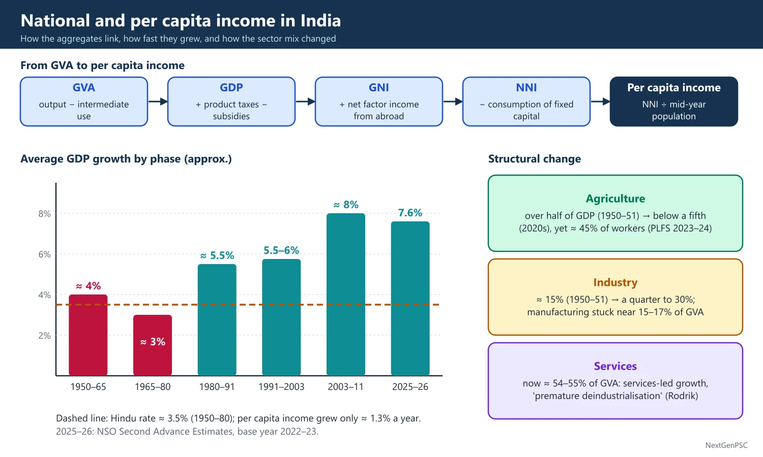
India's national income grew at about 3.5% a year from 1950–51 to 1979–80, the Hindu rate of growth (Raj Krishna), with per capita income rising only about 1.3% a year. Growth rose to about 5.5% in the 1980s and to 6–8% after 1991. The sectoral composition moved from agriculture to services without a large manufacturing phase, the so-called services-led growth pattern.
In simple words
National income is the total value of everything a country produces in a year, and per capita income is that total divided by the population.
Think of a family: total family earnings matter, but what each member gets depends on how many people share it.
India's income grew slowly for thirty years after 1950, then faster after the 1980s and 1991, and most new output came from services rather than factories.
UPSC asks you to explain these growth phases, the sector shift and why it matters for jobs.
1. Concepts and Definitions
GDP and GVA: Gross Domestic Product is the market value of final goods and services produced within the country in a year; Gross Value Added is output minus intermediate consumption, and GDP = GVA + product taxes − product subsidies.
National income (NNI at factor cost): GNI = GDP + net factor income from abroad, and NNI = GNI − consumption of fixed capital; Indian official usage calls per capita NNI at current prices 'per capita income'.
Per capita income: NNI divided by mid-year population; it is an average and hides distribution, which is why Sen and Mahbub ul Haq argued for wider measures such as the HDI (UNDP, 1990).
Constant vs current prices: real growth uses constant prices of a base year so that price changes are removed; nominal values use current prices.
Early estimates: Dadabhai Naoroji gave the first estimate of per capita income (about Rs 20 a year for 1867–68) in Poverty and Un-British Rule in India (1901); V.K.R.V. Rao made the first scientific estimate for 1931–32.
Official system: the National Income Committee (1949), chaired by P.C. Mahalanobis with D.R. Gadgil and V.K.R.V. Rao, laid the base; the CSO (1951), now merged into the National Statistics Office (NSO) under MoSPI, publishes the accounts.
2. Phases of Growth before Liberalisation
1950–51 to 1964–65: GDP grew about 4% a year under the first three Plans, with the Mahalanobis heavy-industry strategy and rising public investment.
1965–66 to 1979–80: wars (1962, 1965, 1971), droughts (1965–67, 1972–73, 1979–80), oil shocks (1973, 1979) and a slowdown in public investment kept growth near 3–3.5%.
Hindu rate of growth: Raj Krishna coined the phrase for the stable 3.5% trend of 1950–80; with population growth of about 2.2%, per capita income grew only about 1.3% a year.
1980s: growth rose to about 5.5% with early liberalisation (Rajiv Gandhi era), rising public spending and borrowing; the fiscal and external imbalances of the late 1980s led to the 1991 crisis.
Debate: Rodrik and Subramanian (2004) argued the take-off began around 1980 with a 'pro-business' turn, while others (e.g. Panagariya, India: The Emerging Giant, 2008) stress the 1991 'pro-market' reforms; the timing of the break is debated.
3. Trends after 1991
Growth acceleration: average growth rose to about 6% in the 1990s and to about 8% in 2003–04 to 2010–11, followed by a slowdown, the COVID-19 contraction of 2020–21 and a recovery.
Latest data: the NSO's First Advance Estimates (7 January 2026) put 2025–26 real GDP growth at 7.4% (6.5% in 2024–25); the Second Advance Estimates (27 February 2026) revised it to 7.6% and moved the accounts to a new base year, 2022–23.
Base years: the series moved 1948–49, 1960–61, 1970–71, 1980–81, 1993–94, 1999–2000, 2004–05, 2011–12 and now 2022–23; each revision updates weights, coverage (e.g. MCA-21 corporate data in 2011–12) and methods.
Per capita income: on the 2011–12 series, per capita NNI at current prices was about ₹1,88,892 in 2023–24 and about ₹2,05,324 in 2024–25 (NSO provisional estimates, May 2025); figures on the new 2022–23 series differ and should be quoted with their series.
Economic Survey 2025–26 (29 January 2026) projected 2026–27 growth at 6.8–7.2% and put potential growth at about 7%.
4. Sectoral Composition and Structural Change
Agriculture: its share of GDP was more than half in 1950–51 and fell to below a fifth by the 2020s, but it still employs about 45% of workers (PLFS 2023–24), so output per worker in farming is far below the average.
Industry: its share rose from about 15% in 1950–51 to about a quarter to 30%; manufacturing has stayed near 15–17% of GVA for decades, far below East Asian peaks of 25–30%.
Services: the largest and fastest-growing sector, now over half of GVA (about 54–55% in recent years), led by IT, finance, trade, transport and public administration.
Kuznets and Clark-Fisher: the classic pattern is a shift from primary to secondary and then tertiary sectors (Colin Clark, 1940; A.G.B. Fisher; Kuznets); India skipped the manufacturing-heavy stage, which Dani Rodrik calls a risk of 'premature deindustrialisation' (2016).
Why services led: skilled English-speaking labour, IT exports after the 1990s, telecom reforms, and constraints on manufacturing such as rigid labour laws, land acquisition and infrastructure gaps (debated).
Consequence: output shifted faster than employment, so labour productivity gaps between sectors persist and good jobs remain scarce for low-skilled workers.
5. Diagrams to Draw
Growth phase chart: draw a bar chart with periods on the x-axis (1950–65, 1965–80, 1980–91, 1991–2003, 2003–11, 2011–20, 2021–26) and average GDP growth on the y-axis; mark the Hindu rate band near 3.5% and the post-2003 peak near 8%.
Structural change chart: draw three lines over time (1950–51 to 2024–25) for the GVA shares of agriculture (falling), industry (rising then flat) and services (rising steeply); label the crossing point when services overtook agriculture (around the late 1970s to 1980s).
Output vs employment shares: draw paired bars for each sector showing share in GVA and share in employment; the large gap for agriculture visually explains low farm productivity.
Lewis two-sector link: sketch the Lewis surplus labour diagram to explain why moving workers out of agriculture raises average productivity.
6. Theory and Debates
Data quality debate: Arvind Subramanian (2019) argued that the 2011–12 series overstated growth by about 2.5 points in 2011–17; the government and the Economic Advisory Council to the PM disputed this; the issue is debated.
Jobless growth: critics argue that services-led growth created too few jobs; others note rising self-employment and construction work; see employment chapter.
Balanced regional growth: per capita income varies widely, with Goa, Sikkim and Delhi far above Bihar and Uttar Pradesh, raising questions of convergence (most studies find divergence across states since the 1990s).
Gujarat vs Bihar example: per capita NSDP in the richest large states is several times that of Bihar, the poorest large state, so national averages hide sharp regional gaps.
China comparison: China's manufacturing share of GDP peaked near a third, while India's stayed near 15–17%, which explains why China absorbed farm labour into factories much faster.
Agriculture's role: farm growth still matters for demand; good monsoons (e.g. 2024) lift rural consumption, while droughts (e.g. 2014 and 2015) depress it.
Informal sector share: the unorganised sector produces roughly half of GVA but employs about nine-tenths of workers, so output data and job data diverge.
GDP vs GNI: India's GNI is slightly below GDP because net factor income from abroad is negative (profit and interest outflows exceed inflows), though remittances count as current transfers, not factor income.
Nominal dollar size: India became the world's fifth largest economy in nominal dollars around 2022 (IMF data) and is projected to move up further; in PPP terms it is third.
Quarterly data: NSO releases quarterly GDP estimates about two months after each quarter, plus advance, provisional and revised annual estimates; quote the vintage you use.
7. Using It in the Exam
10-mark answer (150 words): define national and per capita income, give the three growth phases with figures, one line on sectoral shift and a conclusion on jobs.
15/20-mark answer: add base-year issues, the Rodrik–Subramanian vs 1991 debate, premature deindustrialisation, and a sector share table or chart.
Keywords: Hindu rate of growth, structural transformation, services-led growth, premature deindustrialisation, base year revision, per capita NNI.
Quotable line: Raj Krishna's phrase 'Hindu rate of growth' described the stable 3.5% growth of 1950–80 (paraphrase his view as the structural, not religious, character of slow growth).
| Period | Average GDP growth | Main drivers |
|---|---|---|
| 1950–51 to 1964–65 | About 4% | Plans, public investment, Mahalanobis strategy |
| 1965–66 to 1979–80 | About 3% | Wars, droughts, oil shocks, falling public investment |
| 1980–81 to 1990–91 | About 5.5% | Early deregulation, fiscal expansion, borrowing |
| 1991–92 to 2002–03 | About 5.5–6% | 1991 reforms, services boom |
| 2003–04 to 2010–11 | About 8% | Investment boom, global upswing, credit growth |
| 2025–26 | 7.6% (NSO Second Advance Estimates, Feb 2026, base 2022–23) | Consumption, public capex, services |
Mains points
- Always split the story into phases (1950–65, 1965–80, 1980s, post-1991) and give a growth figure for each.
- Contrast output shares with employment shares: agriculture below a fifth of GVA but about 45% of workers (PLFS 2023–24).
- Mention the base-year change to 2022–23 (February 2026) and say which series a figure comes from.
- Use the premature deindustrialisation argument (Rodrik, 2016) to explain the weak manufacturing share.
- Common mistake: treating per capita income as a welfare measure; add distribution and HDI caveats.
- Draw a simple three-line sector share chart; it earns marks quickly.
Did you know?
- Memory trick for base years since 1993–94: '93, 99, 04, 11, 22' — each about five to eleven years apart.
- Naoroji's per capita income estimate of about Rs 20 a year was the first ever for India and became the core of the drain theory.
Factors Determining National Income and Its Distribution
The level of national income depends on capital accumulation, labour and its skills, technology and productivity, natural resources, and institutions and policy. Its distribution depends on asset ownership (land, capital, education), the structure of employment, wages and the role of the state through taxes and transfers.
In simple words
A country's income grows when it has more machines, more and better-trained workers, better technology and good rules.
It is like a farm: more land and tools, skilled hands and better seeds give a bigger harvest, and who owns the land decides who gets it.
In India, savings and investment, education and health, and policy reforms explain growth, while unequal land and education explain unequal shares.
UPSC asks you to list and explain these factors with Indian data.
1. Concepts and Framework
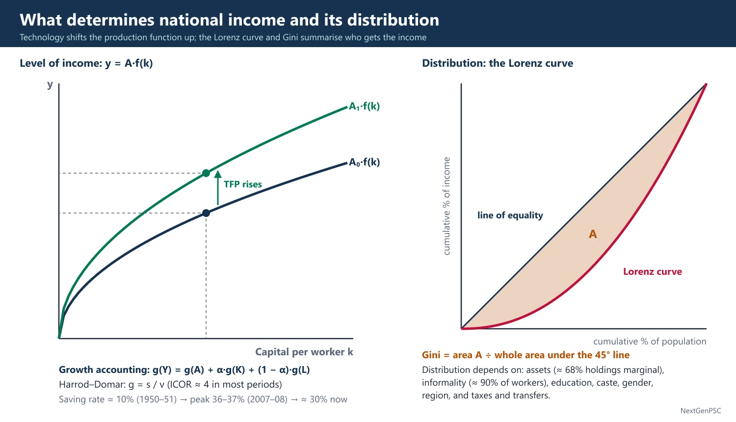
Aggregate production function: Y = A·F(K, L, H, N), where K is physical capital, L labour, H human capital, N natural resources and A total factor productivity (TFP); this frame comes from Solow (1956) and later Mankiw-Romer-Weil (1992) for human capital.
Growth accounting: g(Y) = g(A) + α·g(K) + (1 − α)·g(L), where α is the capital share; the residual g(A) is the Solow residual, a measure of technical progress and efficiency.
Harrod-Domar link: g = s/v, where s is the saving rate and v the incremental capital-output ratio (ICOR); the Indian Plans used this to set investment targets, e.g. the Second Plan's Mahalanobis model.
Functional distribution: the shares of wages, rent, interest and profit in national income (Ricardo, Marx, Kaldor, Kalecki).
Personal distribution: how income is shared among households, measured by the Gini coefficient, quintile shares and the Palma ratio.
2. Factors Determining the Level of National Income
Savings and capital formation: India's gross domestic saving rate rose from about 10% of GDP in 1950–51 to a peak of about 36–37% in 2007–08 and has been near 30% in recent years; the investment rate (GCF) followed a similar path; the ICOR has been about 4 in most periods.
Labour force and demography: the demographic dividend (working-age share rising until about the 2040s) adds labour, but low female labour force participation (about 41.7% for women aged 15 and above in PLFS 2023–24, usual status) limits the gain.
Human capital: literacy rose from 18% (1951) to 74% (Census 2011); health, nutrition and skills raise productivity, as Theodore Schultz (1961) and Gary Becker (1964) argued.
Technology and TFP: studies (e.g. Bosworth and Collins, 2008) find TFP growth contributed a large part of India's post-1980 acceleration, especially in services.
Natural resources and agriculture: monsoon dependence still moves farm output; irrigation covers only about half of net sown area.
Infrastructure: power, roads, ports and digital networks lower costs; public capital expenditure of the Centre rose to about 3.1–3.2% of GDP in recent budgets.
Institutions and policy: property rights, rule of law, macro stability and openness matter (Acemoglu and Robinson, Why Nations Fail, 2012); in India the 1991 reforms, GST (2017) and IBC (2016) are examples.
External sector: trade, FDI and remittances (India is the largest recipient of remittances, about 129 billion US dollars in 2024 per the World Bank) add income and demand.
3. Factors Determining Distribution
Asset distribution: unequal ownership of land (most holdings are marginal, below 1 hectare, about 68% per Agriculture Census 2015–16) and of financial wealth is the root of income inequality.
Employment structure: about 90% of workers are informal (estimates by NCEUS, 2007, and later PLFS-based studies), with low wages and little social security.
Education and skills: returns to higher education are high, so unequal access widens wage gaps (skill-biased technical change).
Caste, gender and region: social exclusion lowers opportunities for SC/ST groups and women; per capita incomes differ several-fold across states.
Functional shift: the wage share in organised manufacturing fell after the 1990s while the profit share rose (ASI data), a trend linked to capital-intensive growth.
State action: progressive taxes, public spending on health and education, the PDS, employment guarantees and direct benefit transfers redistribute income.
4. Theories of Distribution Applied to India
Kuznets (1955): inequality first rises then falls as an economy develops (inverted U); Indian evidence is mixed and the hypothesis is debated.
Kaldor (1956): distribution depends on saving propensities: P/Y = [1/(sₚ − s_w)]·(I/Y) − s_w/(sₚ − s_w); higher investment raises the profit share when capitalists save more.
Kalecki: the degree of monopoly sets the mark-up and hence the profit share; rising market concentration can shift income to profits.
Lewis (1954): with surplus labour, wages stay near subsistence and profits rise until the turning point; useful to explain stagnant rural wages.
Piketty (2014): when r greater than g, wealth concentrates; the World Inequality Lab applied this to India (Chancel, Piketty and others, 2024).
5. Diagrams to Draw
Production function: draw output per worker (y) on the y-axis against capital per worker (k); show a concave curve y = f(k); a rise in TFP shifts the curve up, showing how technology raises income at the same k.
Lorenz curve: draw a square with cumulative share of population on the x-axis and cumulative share of income on the y-axis; draw the 45° line of equality and a bowed Lorenz curve below it; Gini = area between the line and curve divided by the total area under the line.
Kuznets curve: draw per capita income on the x-axis and the Gini on the y-axis with an inverted U shape; mark where India may lie (debated).
6. Indian Evidence and Debates
Investment-led vs consumption-led: the 2003–08 boom was investment-led; after 2011–12 private investment slowed, and recent growth relies on public capex and consumption (Economic Survey 2025–26).
Growth vs distribution: Bhagwati and Panagariya (Why Growth Matters, 2012) argue growth reduces poverty; Drèze and Sen (An Uncertain Glory, 2013) stress public action in health and education; the two views are often called the Bhagwati-Sen debate.
Capital vs labour: India's comparative advantage is in labour, yet growth has been capital- and skill-intensive (e.g. IT, pharmaceuticals, autos); labour-intensive manufacturing is seen as key for broad-based income.
Kerala example: high human development with moderate income shows that public action in health and education can raise wellbeing ahead of income (Drèze and Sen).
Gujarat and Tamil Nadu: strong infrastructure and industrial clusters raised state incomes, showing the role of capital and institutions.
East Asia comparison: Korea and Taiwan combined land reform, mass education and export manufacturing, so growth and equity went together; India lagged in land reform and schooling.
Demographic dividend window: southern states are already ageing while northern states have young populations, so the dividend is regionally uneven.
Policy example: the 2019 corporate tax cut (base rate 22%, 15% for new manufacturing firms) aimed to raise investment, while DBT and free foodgrains support the bottom of the distribution.
Gender factor: raising female labour force participation is often cited as one of the largest possible boosts to India's income (several IMF and McKinsey estimates; magnitudes vary).
7. Using It in the Exam
10-mark answer: list five determinants of national income with one Indian fact each, and three determinants of distribution.
15/20-mark answer: start with Y = A·F(K, L, H), use growth accounting, add Indian saving and investment data, then distribution theories (Kuznets, Kaldor, Lewis) and policy.
Keywords: capital formation, ICOR, TFP, demographic dividend, human capital, informality, asset inequality, Lorenz curve.
Quotable line: Amartya Sen's view that development is the expansion of capabilities (Development as Freedom, 1999) links income to its distribution.
| Factor | Effect on level of income | Effect on distribution | Indian example |
|---|---|---|---|
| Capital formation | Raises output via g = s/v | Raises profit share if capital is concentrated | Saving rate peak about 36–37% (2007–08) |
| Human capital | Raises labour productivity | Narrows gaps if access is equal | Literacy 74% (Census 2011) |
| Technology / TFP | Shifts production function up | Skill-biased change widens wage gaps | IT services boom after 1991 |
| Land and assets | Determines farm output | Unequal holdings mean unequal income | About 68% holdings marginal (Agri Census 2015–16) |
| State policy | Stability and infrastructure | Taxes and transfers redistribute | PDS, DBT, rural job guarantee |
Mains points
- Separate the two halves of the question: factors behind the level of income, and factors behind its distribution.
- Use the production function and growth accounting to give the answer an analytical frame.
- Support each factor with one Indian data point and its year (saving rate, literacy, female LFPR, informality).
- Bring in distribution theories (Kuznets, Kaldor, Lewis, Piketty) to show depth.
- Mention the Bhagwati-Sen debate as a balanced conclusion on growth vs redistribution.
- Draw the Lorenz curve; examiners reward it in distribution answers.
Did you know?
- Memory trick for income determinants: 'K-L-H-A-N-I' — Capital, Labour, Human capital, A (technology), Natural resources, Institutions.
Measuring Poverty in India: Committees, Poverty Lines and Multidimensional Poverty
India measures income poverty with a consumption-based poverty line set by expert groups (Alagh 1979, Lakdawala 1993, Tendulkar 2009, Rangarajan 2014) applied to NSS consumer expenditure data. Since 2014 there has been no official line. The Multidimensional Poverty Index of NITI Aayog (Alkire-Foster method, 12 indicators) and the World Bank's international lines are now widely used.
In simple words
A poverty line is the minimum spending a person needs each month for food and basic needs; people spending less are counted as poor.
It is like a pass mark: below it you fail to meet basic needs.
India's committees changed the line over time, and today poverty is also measured by lack of schooling, health, housing and services, called multidimensional poverty.
UPSC asks you to compare committees and methods and judge which is better.
1. Concepts and Definitions
Absolute poverty: inability to meet a fixed minimum standard of consumption; India uses this approach.
Relative poverty: being far below the typical living standard, e.g. below 50–60% of median income (used in the EU).
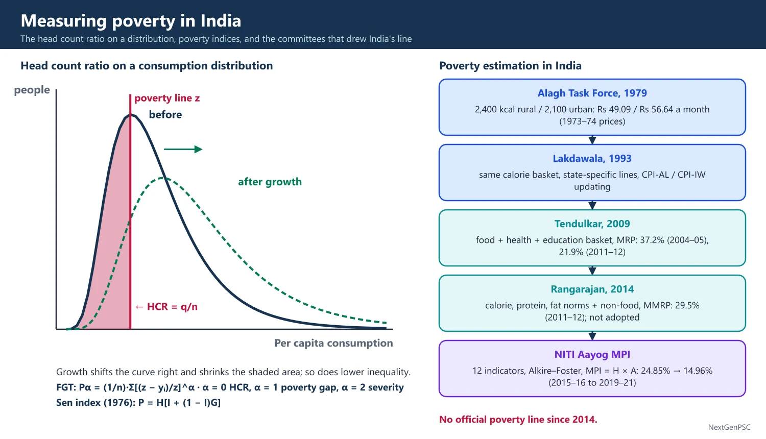
Head Count Ratio (HCR): H = q/n, the share of the population below the poverty line z; simple but ignores how poor the poor are.
Poverty Gap Index: PG = (1/n)·Σ(z − yᵢ)/z over the poor; measures depth.
Squared Poverty Gap and FGT: Foster, Greer and Thorbecke (1984) gave Pα = (1/n)·Σ[(z − yᵢ)/z]^α; α = 0 gives HCR, α = 1 the poverty gap and α = 2 severity, which weights the poorest more.
Sen Index (1976): Amartya Sen combined HCR, the income gap and the Gini among the poor, P = H[I + (1 − I)G], satisfying his monotonicity and transfer axioms.
Capability approach: Sen defines poverty as deprivation of basic capabilities, not just low income, which led to the HDI (1990) and the MPI (Alkire and Foster, 2007–2011; UNDP-OPHI global MPI from 2010).
2. History of Poverty Lines in India
Early estimates: Dadabhai Naoroji's 'subsistence' estimate (1901); the Planning Commission Working Group (1962) proposed Rs 20 per capita per month at 1960–61 prices.
Dandekar and Rath (1971): Poverty in India used 2,250 calories a day and found about 40% rural and 50% urban poverty in 1960–61.
Alagh Task Force (1979): defined the line by calorie norms, 2,400 kcal rural and 2,100 kcal urban, giving Rs 49.09 rural and Rs 56.64 urban per capita per month at 1973–74 prices.
Lakdawala Expert Group (1993): kept the calorie-anchored 1973–74 basket but made state-specific lines and updated them with CPI-AL (rural) and CPI-IW (urban); criticised because the old basket became outdated and calorie intake fell even as incomes rose.
Tendulkar Expert Group (2009): moved away from calorie anchoring to a basket of food, education and health spending, used the urban 2004–05 line as the reference for rural too, used Mixed Reference Period (MRP) data and a price index from NSS unit values; it gave 37.2% poverty in 2004–05 and 21.9% in 2011–12 (Rs 816 rural, Rs 1,000 urban per capita per month in 2011–12).
Rangarajan Expert Group (2014): used a basket meeting calorie, protein and fat norms plus non-food items, separately for rural and urban, with Modified Mixed Reference Period (MMRP) data; it gave 29.5% poverty in 2011–12 (Rs 972 rural, Rs 1,407 urban); the government did not formally adopt it.
Since 2014: no official poverty line; the 2017–18 consumption survey was not released over data-quality concerns; the Household Consumption Expenditure Surveys (HCES) of 2022–23 and 2023–24 restarted the data.
3. Multidimensional Poverty Index
Method: Alkire-Foster counting method; a person is multidimensionally poor if deprived in at least one-third of the weighted indicators; MPI = H × A, where H is the headcount and A the average intensity of deprivation.
NITI Aayog national MPI: three equally weighted dimensions (health, education, standard of living) and 12 indicators, adding maternal health and bank accounts to the 10 global indicators; it uses NFHS data.
Results: the National MPI Progress Review 2023 found the MPI headcount fell from 24.85% (NFHS-4, 2015–16) to 14.96% (NFHS-5, 2019–21), with about 13.5 crore people exiting.
NITI discussion paper (15 January 2024): estimated headcount fell from 29.17% in 2013–14 to 11.28% in 2022–23, with 24.82 crore people moving out; the end points were extrapolated from NFHS trends, so they are projections, not direct survey estimates.
Global MPI (UNDP-OPHI): India reduced the number of multidimensionally poor by about 415 million between 2005–06 and 2019–21 (Global MPI 2023).
4. International Lines and Recent Estimates
World Bank lines: the extreme poverty line was revised in June 2025 to 3.00 US dollars a day at 2021 PPP (from 2.15 dollars at 2017 PPP); lower-middle-income line 4.20 dollars.
India on new line: extreme poverty was about 5.3% in 2022–23 (World Bank, June 2025), down from 27.1% in 2011–12; on the older 2.15 dollar line it was 2.3%; at 4.20 dollars it was about 23.9%.
Comparability caveat: HCES 2022–23 changed questionnaires, recall periods and the number of visits, so comparisons with 2011–12 are not strictly like for like.
Other estimates: SBI Research and others estimated poverty near 4–5% using HCES 2023–24 with the Tendulkar line updated for prices; these are not official.
5. Diagrams to Draw
Poverty line on a distribution: draw the frequency curve of per capita consumption, mark the poverty line z as a vertical line; the area to the left is the HCR; show that a rightward shift of the curve (growth) cuts the HCR, while a narrower curve (less inequality) also cuts it.
Poverty gap: on a chart with people ranked by consumption, shade the gap between z and each poor person's consumption; the shaded area divided by n·z is the poverty gap index.
MPI structure: draw a tree with three dimensions (health, education, living standards) branching into 12 indicators with weights.
6. Debates and Criticisms
Calorie debate: Deaton and Drèze (2009) showed calorie intake fell while real spending rose, so calorie-based lines were unreliable; Patnaik argued calorie deprivation was rising; the debate is unresolved.
Tendulkar line too low: critics called Rs 32 a day urban (2011–12 prices) a starvation line; the Rangarajan group raised it.
Recall period: Uniform (30 days), Mixed and Modified Mixed reference periods give different estimates; the MMRP raises measured consumption and lowers poverty.
Income vs multidimensional: the MPI captures services (sanitation, cooking fuel, bank accounts) that schemes delivered, so it can fall faster than income poverty.
Use of poverty lines: poverty estimates were used to allocate foodgrains to states under the TPDS (1997) and to identify BPL households through BPL censuses (1992, 1997, 2002) and the SECC 2011.
NFSA coverage: the National Food Security Act, 2013 replaced BPL-based targeting with coverage of up to 75% rural and 50% urban population, reducing dependence on the poverty line.
Saxena Committee (2009): advised the Rural Development Ministry on identifying BPL families in rural areas and suggested automatic inclusion and exclusion criteria, later used in SECC 2011.
Hashim Committee (2012): recommended criteria for identifying urban poor households.
Multidimensional examples: Bihar had the highest MPI headcount in NFHS-5 (about a third of the population), while Kerala had below 1% (NITI National MPI 2023).
Global practice: many countries now publish both a monetary line and a national MPI (e.g. Mexico, Colombia), an approach India follows with NITI's MPI.
7. Using It in the Exam
10-mark answer: define poverty line and HCR, list the four committees with one feature each, and mention MPI.
15/20-mark answer: add FGT and Sen index, committee table with 2011–12 figures, the MPI method and results, World Bank 2025 estimates and comparability issues.
Keywords: HCR, poverty gap, FGT, Sen index, MRP/MMRP, Tendulkar, Rangarajan, Alkire-Foster, HCES 2022–23.
Quotable line: Sen's view that poverty is 'capability deprivation' rather than merely low income (Development as Freedom, 1999, paraphrased).
| Committee (year) | Basis of line | Key estimate |
|---|---|---|
| Alagh Task Force (1979) | 2,400 kcal rural, 2,100 kcal urban; 1973–74 prices | Rs 49.09 rural, Rs 56.64 urban per month |
| Lakdawala (1993) | Calorie basket of 1973–74, state-specific, CPI-AL/CPI-IW updating | About 36% poverty in 1993–94 |
| Tendulkar (2009) | Food, health, education basket; MRP; urban line as reference | 37.2% (2004–05); 21.9% (2011–12) |
| Rangarajan (2014) | Calorie, protein, fat norms plus non-food; MMRP | 29.5% (2011–12); not adopted |
| NITI Aayog MPI (2023, 2024) | 12 indicators, Alkire-Foster, NFHS | 14.96% (2019–21); 11.28% (2022–23, projected) |
Mains points
- Present the committees as a timeline with the basis of each line and its estimate.
- Explain HCR, poverty gap and FGT with formulas; examiners reward Sen's axioms and index.
- Distinguish income poverty from multidimensional poverty and say why the MPI falls faster.
- Add the World Bank's June 2025 revision (3 dollars, 2021 PPP; India 5.3% in 2022–23) with the comparability caveat.
- Common mistake: quoting the NITI 2022–23 MPI figure as a survey result; it is a projection.
- Conclude with the need for an official updated poverty line based on HCES data.
Did you know?
- Memory trick for committees in order: 'A-L-T-R' — Alagh, Lakdawala, Tendulkar, Rangarajan (1979, 1993, 2009, 2014).
- In FGT, α works like a magnifying glass: the higher α, the more the poorest are weighted.
Trends in Poverty and Inequality
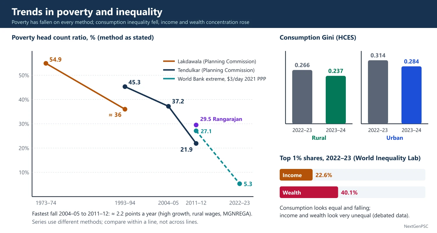
Official poverty fell from about 55% in 1973–74 (Lakdawala method) to 21.9% in 2011–12 (Tendulkar), and recent estimates put extreme poverty near 5% in 2022–23. Consumption inequality measured by HCES fell in 2023–24 (rural Gini 0.237, urban 0.284), but income and wealth inequality estimated by the World Inequality Lab are among the highest in the world.
In simple words
Poverty in India has fallen a lot since the 1970s, especially after 2004, as incomes rose and welfare schemes grew.
But inequality is a different question: it asks how the cake is shared, not just whether the poorest got a bigger slice.
Spending surveys show a fairly equal picture, while income and wealth data show the top 1% holding a very large share.
UPSC asks you to explain these trends, why measures disagree and what policy should do.
1. Poverty Trends: The Long View
1973–74 to 1993–94: on the Lakdawala method, poverty fell from about 54.9% (1973–74) to about 36% (1993–94); the number of poor stayed above 30 crore because of population growth.
1993–94 to 2004–05: the Tendulkar method gives 45.3% (1993–94) to 37.2% (2004–05), a fall of under one point a year despite faster growth, which fuelled the 'growth without poverty reduction' debate of the 1990s.
2004–05 to 2011–12: Tendulkar poverty fell from 37.2% to 21.9% (rural 25.7%, urban 13.7%), about 2.2 points a year, the fastest decline recorded; about 13.8 crore people left poverty.
Why faster after 2004: high growth (about 8%), rising rural wages, construction boom, MGNREGA (2006), better PDS in several states and higher farm prices.
2011–12 to 2022–23: no official estimate; World Bank (June 2025) puts extreme poverty at 27.1% (2011–12) falling to 5.3% (2022–23) on the 3 dollar line; NITI's MPI shows headcount falling to 11.28% (2022–23, projected).
Rural vs urban: rural poverty remains higher, but the gap has narrowed; the rural-urban gap in average MPCE fell from about 84% (2011–12) to about 70% (2023–24) per HCES.
States: Bihar, Jharkhand, Uttar Pradesh, Madhya Pradesh and Chhattisgarh have the highest poverty (both income and MPI); Kerala, Goa, Tamil Nadu and Punjab the lowest.
2. Consumption Inequality
Gini on consumption: NSS data show rural Gini near 0.28–0.29 and urban near 0.35–0.37 in 2011–12 (URP basis); consumption Gini understates inequality because the rich save more and are under-surveyed.
HCES 2022–23 and 2023–24: average MPCE in 2023–24 was ₹4,122 rural and ₹6,996 urban (excluding imputed free items), up from ₹3,773 and ₹6,459 in 2022–23.
Gini fall: HCES shows rural Gini falling from 0.266 (2022–23) to 0.237 (2023–24) and urban from 0.314 to 0.284 (MoSPI fact sheet, 2025).
World Bank: estimated India's consumption Gini at about 25.5 in 2022–23, among the more equal countries on a consumption basis, a claim critics dispute because income data show much higher inequality.
Food share: the share of food in spending has fallen below half in both rural and urban areas, consistent with Engel's law.
3. Income and Wealth Inequality
World Inequality Lab (2024): 'Income and Wealth Inequality in India, 1922–2023: The Rise of the Billionaire Raj' (Bharti, Chancel, Piketty, Somanchi) estimated the top 1% income share at about 22.6% and wealth share at about 40.1% in 2022–23, the highest since the 1920s.
Long trend: the top 1% income share fell from about 20% at Independence to about 6% in the early 1980s and rose steadily after 1991 (World Inequality Lab).
Wealth surveys: the All India Debt and Investment Survey (NSS 77th round, 2019) shows the top 10% of households owning roughly half or more of assets.
Data caveat: WIL combines tax, survey and national accounts data with strong assumptions; critics, including some government economists, say it overstates inequality; it is debated.
Other gaps: gender wage gaps, low female work participation, caste gaps in land and education, and wide inter-state differences.
4. Explaining the Trends
Growth elasticity of poverty: poverty falls faster when growth occurs in sectors where the poor work (agriculture, construction) — Ravallion and Datt (1996) found rural and agricultural growth reduced poverty more than urban growth in India.
Trickle-down debate: Bhagwati and Panagariya argue growth pulled people out of poverty; Drèze and Sen argue public spending on health, education and social security was decisive.
Inequality rising with growth: skill-biased and capital-intensive growth, informality and tax structure explain rising top shares (Kuznets upswing, debated).
Welfare transfers: free foodgrains under PMGKAY (81.35 crore people from January 2024 for five years), PM-KISAN, housing, toilets, cooking gas and DBT reduced deprivation in non-income dimensions.
5. Diagrams to Draw
Poverty trend chart: draw a line graph of HCR on the y-axis against years (1973–74, 1993–94, 2004–05, 2011–12, 2022–23) on the x-axis; mark the Lakdawala, Tendulkar and World Bank series in different line styles and label the steep fall after 2004–05.
Two Lorenz curves: draw consumption (closer to the equality line) and income or wealth (further away) Lorenz curves in one square to show why the measures give different inequality pictures.
Growth incidence curve: draw percentiles on the x-axis and growth of consumption on the y-axis; a downward-sloping curve (bottom grew faster, as HCES 2023–24 suggests) shows pro-poor growth.
6. Theory and Debates
Kuznets hypothesis: India's rising income inequality after 1991 matches the upswing of the inverted U; whether it will turn down is uncertain.
Measurement debate: under-reporting of top incomes in surveys (the gap between NSS consumption and national accounts consumption) inflates measured equality; Deaton and Kozel, The Great Indian Poverty Debate (2005), discuss this for the 1990s.
Pro-poor growth: Kakwani and Pernia define it as growth that benefits the poor proportionally more; HCES 2023–24 shows the bottom 20% gaining faster than the top 20%.
Kerala case: very low poverty and MPI with high remittances and strong public services, though consumption inequality there is above the national average.
Bihar case: fast growth after 2005 from a low base reduced poverty, yet it remains the poorest large state on both income and MPI.
Urban inequality: urban Gini is consistently higher than rural, reflecting skill premiums and asset concentration in cities.
Wage share: the share of wages in net value added of registered factories fell sharply after the early 1990s (ASI), a sign of a functional shift towards profits.
COVID-19 shock: the 2020 lockdown temporarily raised poverty; estimates differ (Pew, World Bank and Azim Premji University gave varying numbers), so quote any figure as an estimate with its source.
Transfers in HCES: HCES 2023–24 also reported MPCE including the imputed value of free items received through schemes (₹4,247 rural, ₹7,078 urban), showing the role of in-kind transfers.
Wealth tax and inheritance: India abolished the wealth tax in 2015 and estate duty in 1985; WIL (2024) suggested a tax on the wealth of the richest families, a proposal that is debated.
Global context: Oxfam reports on Indian billionaires' wealth are widely cited in the media but use different methods; treat them as advocacy estimates.
SDG link: SDG 1 aims to halve poverty in all its dimensions by 2030 and SDG 10 to reduce inequality; NITI's SDG India Index tracks state progress.
7. Using It in the Exam
10-mark answer: give poverty figures for 1973–74, 2004–05, 2011–12 and 2022–23 with the method and source, and one line on inequality.
15/20-mark answer: contrast consumption and income measures, explain causes of decline, use Ravallion-Datt and the Bhagwati-Sen debate, and draw the Lorenz curves.
Keywords: HCR trend, consumption Gini, top 1% share, growth elasticity of poverty, pro-poor growth, Kuznets curve.
Quotable line: Ravallion and Datt's finding that rural growth reduced poverty more than urban growth in India (paraphrased).
| Year | Estimate | Method / source |
|---|---|---|
| 1973–74 | 54.9% | Lakdawala, Planning Commission |
| 1993–94 | 45.3% | Tendulkar, Planning Commission |
| 2004–05 | 37.2% | Tendulkar, Planning Commission |
| 2011–12 | 21.9% (Tendulkar); 29.5% (Rangarajan) | Planning Commission / Expert Group 2014 |
| 2022–23 | 5.3% extreme poverty | World Bank, 3 dollars a day 2021 PPP (June 2025) |
| Measure | Value | Source |
|---|---|---|
| Rural consumption Gini | 0.266 (2022–23) to 0.237 (2023–24) | HCES, MoSPI |
| Urban consumption Gini | 0.314 (2022–23) to 0.284 (2023–24) | HCES, MoSPI |
| Top 1% income share | About 22.6% (2022–23) | World Inequality Lab, 2024 |
| Top 1% wealth share | About 40.1% (2022–23) | World Inequality Lab, 2024 |
Mains points
- Always state the method and source with each poverty figure; mixing Lakdawala and Tendulkar numbers is a common mistake.
- Explain why 2004–12 saw the fastest decline: growth, rural wages, MGNREGA, PDS reforms.
- Show that consumption and income measures of inequality tell different stories, and explain why.
- Use Ravallion-Datt on sectoral growth and poverty to add analytical depth.
- Mention HCES 2022–23 and 2023–24 and the World Bank June 2025 revision for current relevance.
- Conclude on the need for both growth in labour-intensive sectors and public spending on capabilities.
Did you know?
- Between 2004–05 and 2011–12, India's poverty rate fell by about 15 points in just seven years, more than in the previous thirty years together.
UPSC Previous Year Questions: National Income, Poverty and Inequality
From 2014 to 2026 UPSC asked 47 question parts worth 715 marks from this chapter in Paper II. The most-asked topics are national income trends and sectoral composition (15 parts) and trends in poverty and inequality (13 parts), followed by poverty measurement (10) and the factors behind income and its distribution (9). Every question below has a model answer written to the UPSC word limit.
In simple words
Read the question and write your own answer in the time limit first: about 7 minutes for 10 marks and 11 minutes for 15 or 20 marks.
Then compare it with the model answer: did you give figures with year and source, name the committee or economist, and draw the diagram?
Note what you missed, revise that topic in the notes above, and rewrite the answer after a few days.
1. National and Per Capita Income: Patterns, Trends and Sectoral Composition
Example 1 (UPSC 2026, 15 marks): Provide a detailed analysis of the trends in National Income in India since Independence. Discuss the structural changes in the sectoral composition of GDP.
Paper and question: Paper II, Q3(b)
Approach: Trace growth phase by phase with NSO figures, then show how GDP shares moved from agriculture to services and why; use a three-line share chart.
India's national income, compiled by the CSO (now NSO) since 1951 on successive base years (latest 2022–23), shows a long, uneven acceleration.
1950–80: real GDP grew about 3.5% a year, Raj Krishna's 'Hindu rate of growth'; with population growing about 2.2%, per capita income rose only about 1.3%. Wars, the droughts of 1965–67, oil shocks and controls slowed the late 1960s and 1970s. 1980s: growth rose to about 5.5% with early deregulation and fiscal expansion. 1991–2003: about 6% after the reforms; 2003–11: about 8%, an investment boom; then a slowdown, a contraction of about 6% in the COVID year 2020–21 and a recovery to about 7.7% in 2025–26 (NSO provisional estimates on the 2022–23 base).
Structural change: agriculture's share of GDP fell from over half in 1950–51 to about 30% in 1990–91 and about 18% in recent years; industry rose from about 15% to around a quarter and then stagnated, with manufacturing stuck near 15–17%; services rose from about a third to about 55%.
The pattern departs from the Clark-Fisher and Kuznets sequence: India moved from agriculture to services without a manufacturing-led phase. Employment lagged output: agriculture still employs about 46% of workers (PLFS 2023–24), so productivity per farm worker remains low.
Diagram: time (1950–51 to 2025–26) on the x-axis and percentage share of GVA on the y-axis; agriculture line falls, industry line rises then flattens, services line rises steeply and crosses agriculture around 1980.
In sum, growth has risen phase by phase, but the 'missing middle' of manufacturing and the employment-output gap make labour-intensive industrialisation the main task ahead.
Example 2 (UPSC 2025, 20 marks): What is the sectoral composition of India's national income? Mention the most important source of national income in India.
Paper and question: Paper II, Q7(a)
Approach: Define sectoral composition, give shares of primary, secondary and tertiary sectors with year and source, break services and industry into sub-sectors, and name services (especially trade, finance and real estate) as the largest source.
Sectoral composition is the share of each sector in Gross Value Added (GVA), as estimated by the NSO. Following Colin Clark and A.G.B. Fisher, the economy is divided into primary, secondary and tertiary sectors.
Primary sector (agriculture, forestry, fishing, mining): about 18% of GVA for agriculture and allied activities in recent years on the 2011–12 series, down from over half in 1950–51; mining adds about 2%. Within agriculture, livestock and fisheries now contribute a rising share while crops decline.
Secondary sector (manufacturing, construction, electricity, gas and water): about 27–28% of GVA. Manufacturing alone is about 15–17%, construction about 8–9%, utilities about 2–3%. The share has hardly moved since the 1990s, which Rodrik calls a sign of premature deindustrialisation.
Tertiary sector: about 55% of GVA, comprising trade, hotels, transport and communication (about 18–19%); financial services, real estate and professional services (about 22–23%), the single largest sub-group; and public administration, defence and other services (about 12–13%).
Most important source: the services sector is clearly the largest source of national income and has grown fastest since the 1990s, led by IT and business services, finance and telecom. India's services exports reached about 387 billion US dollars in 2024–25 (RBI).
Diagram: a pie chart of GVA with three slices labelled agriculture about 18%, industry about 27%, services about 55%.
Yet agriculture remains the largest source of employment, about 46% of workers in PLFS 2023–24, against its 18% share of output. The new 2022–23 base series, released on 27 February 2026, revised the shares somewhat, so figures should be quoted with their series.
The contrast between output and employment shares shows that raising productivity in farming and expanding labour-intensive manufacturing are needed to make national income growth broad-based.
Example 3 (UPSC 2024, 15 marks): Describe the trend in the growth rate of national income in India from 1950 to 1980 and its impact on poverty.
Paper and question: Paper II, Q3(b)
Approach: Describe growth during 1950–80 by sub-period with reasons, then link slow per capita growth to the persistence of mass poverty, citing estimates of the period.
Between 1950–51 and 1979–80 India's real national income grew at about 3.5% a year, the stable trend that Raj Krishna called the 'Hindu rate of growth'.
1951–65: the first three Plans, the Mahalanobis heavy-industry strategy and rising public investment lifted growth to about 4%, with industry growing about 7% a year till the mid-1960s.
1965–80: growth slipped to about 3% because of the wars of 1962, 1965 and 1971, the droughts of 1965–67, the Plan holiday of 1966–69, the oil shocks of 1973 and 1979, falling public investment and the licence raj.
Per capita income: with population growing about 2.2% a year, per capita income rose only about 1.3% a year, roughly doubling in nearly five decades at that pace.
Impact on poverty: because trickle-down was weak, poverty barely fell. Dandekar and Rath (1971) put about 40% of rural and 50% of urban people below the line in 1960–61; on the Lakdawala method poverty was still about 54.9% in 1973–74.
This failure led to direct anti-poverty programmes: Garibi Hatao (1971), the Minimum Needs Programme of the Fifth Plan, and IRDP (1978–80).
Thus 1950–80 built an industrial base but slow growth, with high population growth and unequal asset ownership, left poverty largely untouched; faster growth after 1980 was needed to reduce it.
Example 4 (UPSC 2024, 10 marks): Is service-led growth in India sustainable? Comment.
Paper and question: Paper II, Q5(b)
Approach: Give the facts of service-led growth, weigh arguments for and against its sustainability (jobs, productivity, exports, AI), and conclude with a balanced view.
Services contribute about 55% of India's GVA but employ only about 30% of workers (PLFS 2023–24), a pattern unlike the manufacturing-led path of East Asia.
For sustainability: services have high and rising productivity; modern services are tradable, and India's services exports reached about 387 billion US dollars in 2024–25 (RBI), financing much of the merchandise trade deficit. Global Capability Centres, digital public infrastructure (UPI, Aadhaar) and a young English-speaking workforce support it. Ghani and Kharas argue services can be a 'new escalator' for growth.
Against: high-end services absorb skilled labour and cannot employ the 46% of workers still in agriculture; most service jobs are informal and low-paid (petty trade, transport). Neglect of manufacturing, Rodrik's premature deindustrialisation, limits jobs for the less educated. AI threatens routine IT and BPO work, and services depend on demand in advanced economies.
Hence service-led growth is sustainable for output but not, by itself, for inclusive employment. Pairing it with labour-intensive manufacturing (PLI, MSME support), skilling and urban services can make it durable.
Example 5 (UPSC 2023, 10 marks): Examine the factors responsible for acceleration in the growth of national income in the decade of 1980s as against 1960s and 1970s.
Paper and question: Paper II, Q1(e)
Approach: Compare growth rates of the 1960s–70s and the 1980s and explain the acceleration through policy, investment, agriculture and fiscal factors, noting the debate on its sustainability.
Real GDP grew about 3–3.5% a year in the 1960s and 1970s but about 5.5% in the 1980s, the first clear break from the 'Hindu rate of growth'.
Policy shift: Rodrik and Subramanian (2004) trace the take-off to an attitudinal, 'pro-business' turn from 1980: delicensing of some industries, broad-banding of licences (1985), relaxed MRTP limits, and easier imports of capital goods and technology under Rajiv Gandhi.
Investment and fiscal push: public investment and government spending rose sharply; the fiscal deficit reached about 8% of GDP by 1990–91. Gross domestic saving rose to about 20% of GDP.
Agriculture and shocks: the Green Revolution spread to rice and new regions; the 1980s had fewer severe droughts (except 1987) and no oil shock like those of the 1970s.
However, part of the growth was debt-financed: rising external commercial borrowing and fiscal deficits ended in the 1991 balance of payments crisis. Panagariya (2008) argues that the 1980s growth was fragile and became sustainable only after the 1991 reforms; the timing of the break is debated.
Example 6 (UPSC 2023, 15 marks): Describe the pattern and trends in national income in India during the pre-economic reform period.
Paper and question: Paper II, Q4(b)
Approach: Describe the level, growth phases, per capita trend and sectoral shifts of national income from 1950–51 to 1990–91, with reasons, using a growth-phase table or chart.
The pre-reform period (1950–51 to 1990–91) saw national income grow under a planned, state-led and inward-looking strategy, with the CSO estimating it from 1951 on the basis laid by the National Income Committee (1949) chaired by P.C. Mahalanobis.
Growth trend: about 4% in 1951–65, about 3% in 1965–80 and about 5.5% in 1980–91; the 1950–80 average of about 3.5% is Raj Krishna's 'Hindu rate of growth'. Growth was volatile: GDP fell in the drought years 1965–66, 1972–73 and 1979–80.
Per capita income: population growth of about 2.2% held per capita income growth to about 1.3% a year up to 1980; it improved to about 3% in the 1980s as growth rose and population growth eased slightly.
Sectoral pattern: agriculture's share of GDP fell from over half in 1950–51 to about 30% in 1990–91; industry rose from about 15% to about a quarter, led by public sector heavy industry; services rose from about a third to over 40%, helped by public administration, banking after the 1969 nationalisation and trade.
Saving and investment: gross domestic saving rose from about 10% of GDP to over 20%, yet growth stayed low because the capital-output ratio rose, reflecting inefficient public enterprises and controls.
Diagram: a bar chart with periods 1951–65, 1965–80 and 1980–91 on the x-axis and average GDP growth on the y-axis (about 4, 3 and 5.5%), with a dashed line at 3.5% for the Hindu rate.
Overall, the pre-reform period built a diversified industrial base and food self-sufficiency, but low productivity, high ICOR and fiscal strains kept growth modest and led to the crisis of 1991.
Example 7 (UPSC 2022, 20 marks): Highlight the major features of National Income trend and its sectoral composition during the last five decades.
Paper and question: Paper II, Q2(a)
Approach: Cover five decades (about 1970s to 2020s) decade by decade for growth, then the sectoral shift and the output-employment mismatch, with data and a share chart.
Over the last five decades India moved from a slow-growing, agrarian economy to one of the fastest-growing large economies, with services as the main engine.
Growth features: (i) acceleration: about 3% in the 1970s, about 5.5% in the 1980s, about 6% in the 1990s, about 8% in 2003–11 and about 6–7% in the 2010s; (ii) reduced volatility, because agriculture's weight fell, so droughts now dent growth less; (iii) shocks: the 1991 crisis, the 2008 global crisis and the COVID contraction of 2020–21 were followed by quick recoveries; (iv) per capita income growth rose from about 1% to about 5% as population growth slowed to about 1% by the 2010s.
Sectoral composition: agriculture's share of GDP fell from about 40% in the early 1970s to about 18% by the early 2020s; industry stayed around a quarter, with manufacturing near 15–17%; services rose from about a third to over half.
Drivers: services boomed with IT, telecom and financial reforms after 1991; industry was held back by infrastructure, labour and land constraints; agriculture's slower growth (about 3%) relative to the economy lowered its share.
Employment mismatch: agriculture's share in employment fell much more slowly, from about 74% (1972–73, NSS) to about 46% (PLFS 2023–24), so the income gap between farm and non-farm workers widened.
Diagram: three lines of GVA shares from 1970–71 to 2022–23; agriculture falling, services rising and overtaking agriculture around 1980, industry nearly flat.
The trend shows faster and steadier growth but a lopsided structure; inclusive growth needs manufacturing jobs, higher farm productivity and better skills.
Example 8 (UPSC 2021, 20 marks): Do you think that India experienced a major break in GDP growth and its sectoral composition during the 1980s? Give reasons.
Paper and question: Paper II, Q4(a)
Approach: Take a position (yes, a growth break around 1980, though debated), give evidence on growth and sectoral shares, explain the reasons, and present the counter-view that 1991 was the real break.
Statistical studies (Wallack, 2003; Rodrik and Subramanian, 2004; Virmani) locate a structural break in GDP growth around 1980–81, so the answer is broadly yes, though its nature is debated.
Evidence of a growth break: average growth rose from about 3.5% in 1950–80 to about 5.5% in 1980–91; per capita income growth more than doubled, from about 1.3% to about 3%. Industrial growth recovered to about 7–8% a year from the stagnation of 1965–80.
Sectoral break: services accelerated to about 6.5–7% a year and overtook agriculture as the largest sector around 1980; agriculture's share fell from about 36% to about 30% during the decade, and the Green Revolution spread to rice in eastern India.
Reasons: (i) the 'pro-business' policy turn under Indira Gandhi (1980) and Rajiv Gandhi: partial delicensing, broad-banding (1985), MRTP relaxation, easier technology imports; (ii) a large fiscal stimulus, with the fiscal deficit near 8% of GDP; (iii) a rise in saving and investment; (iv) better monsoons and no oil shock; (v) the spread of telecom and banking services.
Counter-view: Panagariya (2008) and Ahluwalia argue the 1980s growth rested on unsustainable fiscal and external borrowing that culminated in the 1991 crisis, and that the true, durable break came with the 1991 'pro-market' reforms, when trade, industrial and financial liberalisation lifted growth to 6–8% for two decades.
Diagram: log of real GDP on the y-axis against years 1950–2000; two fitted trend lines, a flatter one up to 1980 and a steeper one after, with the kink marked at 1980.
Thus India did experience a break in growth and sectoral composition in the 1980s, but it became robust only when backed by the structural reforms of 1991.
Example 9 (UPSC 2020, 15 marks): Discuss the changes in sectoral composition of GDP with the changes in the sectoral components of employment in India since Independence.
Paper and question: Paper II, Q4(b)
Approach: Set the output shares against the employment shares of the three sectors from 1951 to recent years, explain the lag using the Clark-Fisher and Lewis frameworks, and draw out implications.
The Clark-Fisher hypothesis expects labour to move from primary to secondary and tertiary sectors along with output. India's experience shows a shift in output far faster than in employment.
Output: agriculture's share of GDP fell from over half in 1950–51 to about 30% in 1990–91 and about 18% recently; industry rose from about 15% to about 27%; services from about a third to about 55%.
Employment: agriculture employed about 72% of workers in 1951 (Census), about 64% in 1993–94 (NSS), about 49% in 2011–12, and about 46% in 2023–24 (PLFS). Industry's share rose to about a quarter, mostly in construction rather than manufacturing; services employ about 30%.
Why the lag: (i) capital-intensive industrial strategy under the Mahalanobis model created few jobs; (ii) services growth was skill-intensive (IT, finance); (iii) rigid labour laws and small firm size limited formal manufacturing jobs; (iv) low education and skills kept rural workers in farming. In Lewis's (1954) terms, surplus labour was not absorbed.
Recent reversal: agriculture's employment share rose from about 42.5% in 2018–19 to about 46% in 2023–24, partly due to the COVID-19 return migration and more women counted as unpaid helpers.
Diagram: two stacked bars for 1951 and 2023–24, one for GDP shares and one for employment shares, showing agriculture's output share shrinking far more than its employment share.
Implications: output per worker in agriculture is about a third of the economy-wide average, causing rural poverty and disguised unemployment; inclusive growth needs labour-intensive manufacturing, rural non-farm jobs and skilling.
Example 10 (UPSC 2019, 10 marks): Examine the trends in GDP at factor cost during the pre-reform period in India.
Paper and question: Paper II, Q5(c)
Approach: Define GDP at factor cost, then give its growth trend by phase from 1950–51 to 1990–91, with volatility and reasons.
GDP at factor cost is the value of goods and services produced within the country, measured as the sum of factor incomes, that is GDP at market prices minus net indirect taxes; it was India's headline measure until the 2011–12 series moved to GVA at basic prices in 2015.
1950–65: GDP at factor cost grew about 4% a year as Plan investment expanded industry, power and irrigation. 1965–80: growth fell to about 3% because of wars, droughts (GDP fell in 1965–66, 1972–73 and 1979–80), oil shocks, declining public investment and licence-raj inefficiency. Raj Krishna called the 1950–80 average of about 3.5% the 'Hindu rate of growth'.
1980–91: growth rose to about 5.5% with partial deregulation, higher public spending and the spread of the Green Revolution.
Features: per capita GDP grew only about 1.3% until 1980; agriculture's share fell from over half to about 30%; growth was volatile because of monsoon dependence. The late-1980s acceleration was debt-financed and ended in the 1991 crisis.
Example 11 (UPSC 2018, 20 marks): Reflect on issues and implications of structural transformation in India's national income.
Paper and question: Paper II, Q3(a)
Approach: Define structural transformation, describe India's output and employment shifts, then discuss issues (missing manufacturing, informality, productivity gaps) and implications (jobs, inequality, sustainability).
Structural transformation is the reallocation of output and labour from low-productivity agriculture to higher-productivity industry and services; Kuznets, Clark and Chenery documented it as a core feature of modern growth.
India's path: agriculture's share of GDP fell from over half (1950–51) to about 18% (2016–17), services rose to over half, while industry stagnated around 27–30% and manufacturing at about 16%. India thus leap-frogged from agriculture to services.
Issue 1, premature deindustrialisation: manufacturing's share peaked at a much lower income level than in East Asia, as Rodrik (2016) notes, so the classic route of absorbing unskilled labour in factories is weak.
Issue 2, slow labour shift: agriculture still employed nearly half the workforce (about 49% in 2011–12, NSS), so labour productivity there is roughly a third of the average; disguised unemployment persists.
Issue 3, informality and dualism: over 90% of workers are informal; growth has come from capital- and skill-intensive formal firms, while a large tail of tiny, low-productivity enterprises remains (the 'missing middle').
Implications: (i) jobless or job-poor growth, especially for youth and women (female LFPR was about 23% in PLFS 2017–18); (ii) widening rural-urban and inter-state inequality; (iii) dependence of the services-led model on skilled labour and external demand; (iv) fiscal pressure for farm support.
Diagram: sectoral shares of GDP and employment plotted together against time; the agriculture GDP line falls steeply, the agriculture employment line falls slowly, and the widening wedge between them shows the productivity gap.
Policy responses include Make in India (2014), labour code reform, MUDRA loans and skilling. Transformation that moves workers into productive non-farm jobs is the key to inclusive growth.
Example 12 (UPSC 2017, 10 marks): Relative contribution of agriculture to the GDP of India has been going down steadily since Independence. Do you think this highlights a weakness of the economy? Explain.
Paper and question: Paper II, Q5(a)
Approach: Explain that a falling agricultural share is a normal sign of development (Clark-Fisher, Kuznets), then show where it does reveal weakness in India (employment share, productivity, missing manufacturing).
Agriculture's share of India's GDP fell from over half in 1950–51 to about 17–18% by 2016–17.
Not a weakness in itself: as Engel's law, Clark-Fisher and Kuznets show, the demand for food grows more slowly than income, so every developing economy sees agriculture's share fall; in the US it is about 1%. Farm output itself grew about 2.5–3% a year, and India became self-sufficient in foodgrains after the Green Revolution.
Where it signals weakness: (i) the employment share fell far more slowly; about 49% of workers were still in agriculture in 2011–12 (NSS), so output per farm worker is a fraction of non-farm output and rural incomes lag; (ii) the labour leaving farming went mainly to construction and informal services, not manufacturing; (iii) farm growth is volatile and monsoon-dependent, and public investment in agriculture fell after the 1980s.
Hence the decline itself reflects development, but the slow shift of workers and low farm productivity reveal a structural weakness that calls for agricultural productivity growth and non-farm job creation.
Example 13 (UPSC 2017, 15 marks): How did per capita income in India behave since Independence? Has it improved the well-being of the people uniformly? Give specific reasons.
Paper and question: Paper II, Q8(c)
Approach: Trace per capita income growth phase by phase, then answer the second part (no, not uniformly) with evidence on inter-state, rural-urban, class and social-group disparities and their reasons.
Per capita income, net national income divided by population, is the common average measure of living standards.
Behaviour: it grew only about 1.3% a year in 1950–80, as GDP grew about 3.5% and population about 2.2%; about 3% in the 1980s; about 4% in the 1990s; and about 6–7% in 2003–11, as growth rose and population growth slowed.
Not uniform, because: (i) inter-state gaps: per capita income in Goa or Delhi is several times that of Bihar,; (ii) sectoral gaps: agriculture employs about half the workforce but earns under a fifth of GDP; (iii) rural-urban gaps: urban per capita consumption was about 84% higher than rural in 2011–12 (NSS); (iv) class inequality: the top 1% income share rose from about 6% in the early 1980s to over 20% by 2014 (Chancel and Piketty, 2017); (v) social groups: SCs, STs and women lag in assets, education and wages.
Well-being: poverty fell from about 45% (1993–94) to about 22% (2011–12, Tendulkar), and literacy and life expectancy improved, but malnutrition remained high (NFHS-4, 2015–16: about 38% of children stunted).
Reasons: unequal land and asset ownership, skill-biased services growth, jobless organised industry, regional gaps in infrastructure and governance, and social discrimination.
Per capita income has risen substantially, but well-being has improved unevenly; as Sen argues, capabilities such as health and education must improve along with average income.
Example 14 (UPSC 2016, 15 marks): Discuss the changes in the sectoral composition of GDP in recent years.
Paper and question: Paper II, Q8(c)
Approach: Use the 2011–12 series (GVA at basic prices) to show recent sectoral shares and growth rates, explain the changes, and assess them.
Since the 2011–12 base revision of January 2015, the CSO measures sectoral output as GVA at basic prices, which shows a continuing shift towards services.
Agriculture: its share of GVA fell from about 18.5% in 2011–12 to about 17–18% by 2015–16 at current prices; growth was erratic, with consecutive droughts in 2014–15 and 2015–16 pulling farm growth below 1%.
Industry: about 30–31% of GVA in 2011–12, edging down; manufacturing was about 17–18%, and its growth was revised upward in the new series because it uses MCA-21 corporate data, a point debated by analysts. Mining and construction slowed with the investment slump and stalled projects.
Services: rose from about 49% to about 53% of GVA, led by financial, real estate and professional services, trade, transport and communication; public administration grew with government spending.
Causes: rising incomes raised demand for services (Engel effect); IT, telecom and finance gained productivity; industry suffered from the twin balance sheet problem of stressed firms and banks; agriculture faced weather shocks.
Diagram: a stacked bar for 2011–12 and one for 2015–16, each divided into agriculture, industry and services, with the services segment visibly larger in the later bar.
The recent changes deepen the services-led pattern; policies such as Make in India (2014) aim to raise manufacturing to 25% of GDP, a goal not yet achieved.
Example 15 (UPSC 2014, 15 marks): Highlight the structural changes in Indian economy before 1991.
Paper and question: Paper II, Q3(b)
Approach: Describe structural change before 1991 under output composition, employment, ownership (public sector), saving-investment and trade, with reasons and limits.
Structural change means a lasting shift in the composition of output, employment, ownership and trade; planned development before 1991 produced several such shifts.
Output composition: agriculture's share of GDP fell from over half to about 30%; industry rose from about 15% to about a quarter; services rose from about a third to over 40%. Within industry, capital goods, steel, chemicals and engineering grew relative to textiles and food processing, as the Mahalanobis strategy intended.
Employment: agriculture's share in the workforce fell only from about 72% (1951) to about 64% (1993–94), so structural change in jobs lagged.
Ownership: the public sector expanded to the 'commanding heights' under the Industrial Policy Resolution of 1956; bank nationalisation (1969 and 1980) and coal nationalisation (1971–73) widened state control; public sector share in GDP rose to about a quarter by 1990–91.
Saving, investment and infrastructure: the gross domestic saving rate rose from about 10% to over 20% of GDP; irrigation, power and railways expanded; the Green Revolution made India self-sufficient in foodgrains.
Trade: import substitution kept the trade-to-GDP ratio low; exports diversified from jute, tea and cotton textiles towards engineering goods, gems and garments, but India's share in world exports fell from about 2% in 1950 to about 0.5% by 1990.
Limits: high capital-output ratios, protected but inefficient industry and fiscal deficits created too few jobs and led to the 1991 crisis and market-oriented reforms.
2. Factors Determining National Income and Its Distribution
Example 16 (UPSC 2023, 15 marks): What are the factors contributing towards shift in sectoral composition in Gross National Product (GNP) in India during the pre-economic reform period? Discuss.
Paper and question: Paper II, Q2(b)
Approach: Explain the shift in GNP shares before 1991 through demand-side (Engel's law), supply-side (productivity, investment) and policy factors (Mahalanobis strategy, public sector).
Between 1950–51 and 1990–91 agriculture's share of national product fell from over half to about 30%, industry's rose from about 15% to about a quarter and services' from about a third to over 40%. Several factors drove this shift.
Demand side: by Engel's law, as per capita income rose, the share of food in spending fell and demand for manufactures and services rose faster; urbanisation (17% in 1951 to about 26% in 1991) added to it.
Planning strategy: the Mahalanobis model of the Second Plan (1956–61) put heavy industry first; the Industrial Policy Resolution of 1956 reserved basic industries for the public sector, which built steel, power, heavy engineering and chemicals.
Investment and saving: the saving rate rose from about 10% to over 20% of GDP, financing industrial capital formation; public investment in railways, irrigation and power expanded the secondary sector.
Slow farm growth: agriculture grew only about 2.5% a year owing to unfinished land reforms, monsoon dependence and limited irrigation; the Green Revolution after 1966 helped mainly wheat in the north-west, so its share fell faster.
Expansion of services: government administration and defence grew with the state; bank nationalisation (1969) spread branch banking; trade, transport and communication grew with industry.
Thus income-driven demand, planned industrialisation and state-led services caused the shift, though employment did not follow output, leaving a large low-productivity farm workforce.
Example 17 (UPSC 2023, 20 marks): Explain the main causes of inequality in income distribution in India and examine how it affects welfare of the society.
Paper and question: Paper II, Q4(a)
Approach: Give the extent of inequality with data, explain its main causes (assets, education, labour market, regional, social, policy), then show its welfare effects using a Lorenz curve and the diminishing marginal utility argument.
Income inequality in India is high and rising: the World Inequality Lab (2024) estimates that the top 10% received about 57.7% and the top 1% about 22.6% of national income in 2022–23, while consumption Gini from NSS surveys is far lower because the rich are under-sampled.
Causes: (i) unequal assets: concentrated land and financial wealth; about 68% of land holdings are marginal (Agriculture Census 2015–16); (ii) human capital gaps: unequal access to quality education and health makes returns to skill uneven; (iii) labour market dualism: about 90% of workers are informal, while skill-biased growth in IT and finance raises top salaries; (iv) falling labour share: capital-intensive growth raised profits relative to wages; (v) regional imbalance: per capita income in rich states is several times that in Bihar; (vi) social exclusion by caste and gender; (vii) a tax system dependent on indirect taxes.
Welfare effects: by the Pigou-Dalton principle and diminishing marginal utility, a transfer from rich to poor raises total welfare, so high inequality lowers social welfare for a given income; Atkinson's equally distributed equivalent income formalises this.
Inequality also reduces welfare by slowing poverty reduction, limiting the poor's investment in education (credit constraints), weakening aggregate demand, and creating social conflict and elite capture of policy.
Diagram: cumulative share of population on the x-axis and cumulative share of income on the y-axis; the 45° line is perfect equality; a bowed Lorenz curve shows inequality, and the Gini coefficient equals the area between the line and the curve divided by the whole triangle.
Policies such as universal health and education, progressive taxation, DBT and rural employment can reduce inequality and raise welfare without hurting growth.
Example 18 (UPSC 2021, 15 marks): Examine the relative role of demand side factors in determining national income in India.
Paper and question: Paper II, Q4(b)
Approach: Explain the Keynesian demand-side view (Y = C + I + G + X − M), give India's demand composition with data, assess each component's role, and contrast it with supply constraints.
Keynes's principle of effective demand holds that in the short run output is set by aggregate demand, Y = C + I + G + (X − M), when there is spare capacity; in the long run supply factors (capital, labour, technology) dominate.
Private consumption (PFCE) is close to 60% of India's GDP and the most stable driver; rural demand depends on monsoons and farm incomes. Its weakness in 2019–20 and during COVID-19 dragged growth down.
Investment (GFCF about 30–34% of GDP) was the engine of the 2003–08 boom, when it rose to about 35%; after 2011–12 private investment slowed because of the twin balance sheet problem, and since 2020 public capital expenditure has led.
Government consumption (about 10–11% of GDP) acts counter-cyclically, as in the 2020–21 relief packages.
Net exports are usually negative (merchandise deficit), but services exports and remittances support demand; the 2003–08 boom also benefited from global demand.
Relative role: demand factors explain the cycles (2008 slowdown, 2019–20 slump, post-COVID recovery), but India's long-run growth has been constrained more on the supply side: infrastructure, skills, land and productivity. Inflation when demand outruns supply, as in 2010–13, shows this limit.
Example 19 (UPSC 2016, 20 marks): What is 'Crony Capitalism'? Is it true that almost all Developing Countries are facing the threat of 'Crony Capitalism' in their development efforts?
Paper and question: Paper II, Q4(a)
Approach: Define crony capitalism, explain how it arises and its costs, give evidence from developing countries including India, and judge whether 'almost all' face the threat.
Crony capitalism is a market economy in which business success depends on close relationships with politicians and officials rather than on efficiency, through favourable licences, contracts, tax breaks, natural-resource allocations and regulatory protection. It is a form of rent-seeking, analysed by Anne Krueger (1974) and Jagdish Bhagwati's 'directly unproductive profit-seeking' (1982).
How it arises: weak institutions, discretionary state control over scarce resources (land, spectrum, mines), opaque political finance, and the capture of regulators. Liberalisation without strong regulation can shift rents from licences to resources.
Costs: misallocation of capital to connected firms, entry barriers, lower competition and innovation, bad loans in state banks, higher inequality and loss of public trust; Acemoglu and Robinson (2012) call such arrangements 'extractive institutions'.
Evidence: The Economist's crony-capitalism index (2014, 2016) ranked Russia, Malaysia, the Philippines, Ukraine and India among the most exposed countries. In India, the 2G spectrum case and the coal block allocations, cancelled by the Supreme Court in 2014, showed discretion favouring connected firms; Raghuram Rajan warned in a 2008 speech of a threat of oligarchy. Indonesia under Suharto, and the role of cronyism in the 1997 East Asian crisis, are other examples.
Is the threat universal? Many developing countries face it because state discretion is large and institutions are weak, but it is not inevitable: Chile, Botswana and South Korea after 1997 reduced cronyism through auctions, competition law and transparency. Developed countries are not immune either (US lobbying).
India has responded with spectrum and coal auctions, the Insolvency and Bankruptcy Code (2016), the Competition Commission (2003) and electoral bond judgement of 2024 striking down opaque political funding. Strong institutions, not the size of the state, decide whether cronyism grows.
Example 20 (UPSC 2015, 20 marks): Explain the major factors that affected the growth rate of the economy in post-independence India till 1991.
Paper and question: Paper II, Q2(b)
Approach: Divide 1950–91 into phases and explain the factors that raised or depressed growth: saving and investment, strategy and controls, agriculture and weather, shocks, fiscal and external factors.
India's GDP grew about 3.5% a year from 1950 to 1980 and about 5.5% in the 1980s. The main factors behind this record can be grouped as follows.
Saving and capital formation: the saving rate rose from about 10% to over 20% of GDP, but growth did not rise in proportion because the incremental capital-output ratio climbed from about 3 in the 1950s to about 5 by the 1970s (by Harrod-Domar, g = s/v), reflecting inefficient use of capital.
Development strategy: the Mahalanobis heavy-industry strategy built a capital goods base but neglected wage goods and labour-intensive industry; import substitution and the licence raj (Industries Act, 1951; MRTP Act, 1969) protected inefficient firms and reduced competition, as Bhagwati and Desai (1970) showed.
Agriculture and weather: agriculture, about half of GDP, grew about 2.5%; incomplete land reforms limited productivity; droughts in 1965–67, 1972–73, 1979–80 and 1987 caused sharp falls. The Green Revolution from 1966 raised foodgrain output and stabilised growth.
Shocks: wars (1962, 1965, 1971), the devaluation crisis of 1966, the Plan holiday (1966–69) and oil shocks (1973, 1979) depressed growth in 1965–80. Public investment, especially in infrastructure, slowed after 1965, which Isher Ahluwalia linked to industrial stagnation.
Population: growth of about 2.2% a year reduced per capita gains to about 1.3%.
1980s revival: partial deregulation, technology imports, higher public spending and better harvests raised growth, but large fiscal deficits (about 8% of GDP) and external borrowing made it unsustainable, ending in the 1991 crisis.
Hence low efficiency of investment, controls and agricultural fragility mattered more than a lack of saving in restraining growth until 1991.
Example 21 (UPSC 2015, 20 marks): How does population growth affect economic development of a country? Can the age structure of population alter the pattern of development in a country? Examine in the light of the Indian experience.
Paper and question: Paper II, Q3(a)
Approach: Present the pessimistic (Malthus, Coale-Hoover) and optimistic (Kuznets, Simon) views, then explain how age structure creates a demographic dividend, applying it to India with Census and NFHS data.
Population growth affects development through saving, investment, labour supply, demand and pressure on resources; economists disagree on the net effect.
Pessimistic view: Malthus (1798) argued that population outruns food supply. Coale and Hoover (1958), using India as their case, argued that rapid population growth raises the dependency burden, lowers per capita saving and diverts investment to housing and schools. If GDP grows 3.5% and population 2.2%, per capita income rises only 1.3%, as in India in 1950–80.
Optimistic view: Kuznets and Julian Simon (1981) argued that a larger population brings more ideas, scale economies and market size; Boserup (1965) showed population pressure can induce agricultural innovation.
Age structure: yes, it alters the pattern. When fertility falls after mortality (the demographic transition), the share of the working-age population (15–64) rises and the dependency ratio falls, creating a demographic dividend: more workers, higher saving and more female participation. Bloom and Williamson attribute about a quarter to a third of East Asia's 'miracle' growth to this.
Indian experience: population grew about 2.2% a year till the 1980s, which held back per capita income. Since the 1990s fertility has fallen (TFR about 2.2 in NFHS-4, 2015–16) and the working-age share is above 60%; Aiyar and Mody (2011, IMF) found that the dividend explained a significant part of the growth acceleration since the 1980s. The dividend is expected to peak around the 2040s.
Conditions: the dividend needs jobs, skills, health and female labour force participation, which is low in India; southern states are already ageing while Bihar and Uttar Pradesh remain young.
Hence age structure and human capital, more than size, decide whether population becomes a burden or a dividend.
Example 22 (UPSC 2015, 15 marks): The 'dichotomy of development' in India emerged owing to 'governance deficit' and 'crony capitalism'. Examine.
Paper and question: Paper II, Q3(c)
Approach: Define dichotomy of development (dualism between sectors, regions and groups), explain how governance deficit and crony capitalism produced it, and add the other structural causes for balance.
The dichotomy of development refers to India's dual pattern: a modern, high-productivity, globally connected segment (IT, finance, large firms, metros) coexisting with a vast low-productivity segment (small farms, informal enterprises, backward regions). It echoes Boeke's dualism and Lewis's dual economy.
Governance deficit: weak delivery of public goods (health, education, police, courts) means the poor cannot convert growth into capabilities; leakages in the PDS (estimated at over 40% in 2011–12 by some studies), absenteeism of teachers and doctors, and slow courts raise costs for small firms. Rajiv Gandhi's remark that only about 15 paise of each rupee reached the poor captured this.
Crony capitalism: discretionary allocation of land, spectrum, coal and mines (2G and coal block cases, cancelled in 2012 and 2014) channelled rents to connected firms; state bank lending to them led to bad loans, crowding out credit for small enterprises.
Other causes: skill-biased services growth, unequal land ownership, regional differences in infrastructure, and capital-intensive industrialisation also created dualism, so governance and cronyism are important but not the only causes.
Remedies include auctions, DBT and JAM (2014 onwards), the IBC (2016), and investment in public services; better governance can make growth inclusive.
Example 23 (UPSC 2014, 15 marks): In Indian economy, dichotomy of development emerged during the pre-reform period despite efforts of holistic development. Delineate the factors responsible for it.
Paper and question: Paper II, Q4(c)
Approach: Define the dichotomy (dualism) of the pre-reform period, recall the holistic aims of planning, and delineate the factors (strategy, land, technology, regional and social) that produced it.
Planning aimed at holistic development: growth with self-reliance, social justice and a 'socialistic pattern of society' (Avadi resolution, 1955). Yet a dichotomy emerged between a modern, organised, capital-intensive sector and a large traditional, unorganised sector, between regions and between social groups.
Development strategy: the Mahalanobis model favoured heavy, capital-intensive industry; the organised sector employed under a tenth of workers, while most remained in agriculture and household industry, producing Lewis-type dualism.
Agrarian structure: land reforms abolished intermediaries but ceiling and tenancy laws were poorly implemented, so land stayed concentrated; the Green Revolution (from 1966) favoured irrigated, larger farms in Punjab, Haryana and western Uttar Pradesh, widening regional and class gaps.
Regional factors: freight equalisation (1952) removed the advantage of mineral-rich eastern states, and investment clustered in already developed areas; Myrdal's backwash effects operated.
Social and institutional: caste, gender and illiteracy limited access to education and credit; benefits of subsidies and nationalised bank credit were captured by the better-off; licensing favoured large houses, as the Hazari report (1967) and the Dutt Committee (1969) found.
Hence strategy choices, unequal assets and weak institutions caused the dichotomy despite holistic aims, which later shaped the 'inclusive growth' agenda of the Eleventh Plan.
Example 24 (UPSC 2014, 20 marks): 'Elitist bias' and 'crony capitalism' have eclipsed the issues of efficiency and distributive justice in India. Elaborate.
Paper and question: Paper II, Q7(a)
Approach: Define elitist bias and crony capitalism, show with Indian examples how they distort efficiency (allocation) and distributive justice (equity), and suggest institutional remedies.
Elitist bias means public policy and spending tilted towards the interests of the well-off (urban middle class, large farmers, organised workers, big business), a theme in Michael Lipton's 'urban bias' (1977) and Pranab Bardhan's account of India's 'dominant proprietary classes' (1984). Crony capitalism means business success through political connections rather than efficiency.
Elitist bias in practice: higher education and urban hospitals received relatively more public money than primary schools and rural health; subsidies on power, fertiliser and LPG went disproportionately to better-off households; MSP and procurement benefited mainly large farmers in a few states; the Economic Survey 2015–16 estimated that a large share of small savings and other subsidies went to the rich ('bounties for the well-off').
Crony capitalism in practice: discretionary allocation of spectrum (2G, 2008) and coal blocks (cancelled by the Supreme Court in 2014), land acquisition on favourable terms, and loans from public sector banks to connected firms led to large non-performing assets.
Effect on efficiency: resources go to connected rather than productive firms, competition and innovation fall, entry barriers rise, bad loans crowd out credit to MSMEs, and rent-seeking (Krueger, 1974) wastes resources. Allocative efficiency, in the Pareto sense, is lost.
Effect on distributive justice: rents accrue to a narrow group; the top 1% income share rose steadily after 1991 (World Inequality Lab); public services for the poor remain under-funded, and trust in markets falls, which Raghuram Rajan and Luigi Zingales warned can create a backlash against reform.
Remedies: auctions for natural resources (spectrum and coal since 2014–15), DBT to target subsidies, the IBC (2016), stronger regulators, transparent political funding, and higher spending on primary health and education.
Hence elitist bias and cronyism undermine both efficiency and equity; transparent, rule-based institutions restore both.
3. Measuring Poverty in India: Committees, Poverty Lines and Multidimensional Poverty
Example 25 (UPSC 2026, 10 marks): What are the different methods of measurement of poverty in India? Which one do you think is most appropriate and why?
Paper and question: Paper II, Q1(e)
Approach: List the methods (calorie-based lines, Tendulkar, Rangarajan, MPI, World Bank lines) briefly, then argue for the most appropriate (a consumption line plus MPI as complement) with reasons.
Poverty in India has been measured mainly by consumption-based poverty lines from NSS surveys, and more recently by multidimensional indices.
Methods: (i) calorie-anchored lines: Alagh Task Force (1979), 2,400 kcal rural and 2,100 kcal urban, and Lakdawala (1993) with state-specific price updating; (ii) Tendulkar (2009): a basket of food, education and health spending on MRP data, giving 21.9% in 2011–12; (iii) Rangarajan (2014): calorie, protein and fat norms plus non-food items, giving 29.5%.
Newer measures: (iv) NITI Aayog's National MPI: 12 indicators of health, education and living standards (Alkire-Foster); (v) World Bank lines: 3 dollars a day (2021 PPP), giving 5.3% in 2022–23.
Most appropriate: a consumption-based line on the HCES 2022–23 data, updated for a modern basket like Rangarajan's, is best for tracking income poverty, while the MPI captures deprivations in schooling, health and housing that income misses, in line with Sen's capability approach. Using both together, a 'dashboard', is most appropriate because income and non-income deprivation do not always overlap.
Example 26 (UPSC 2025, 20 marks): What are the methods used in measuring poverty and inequality in India? Analyse.
Paper and question: Paper II, Q4(a)
Approach: Explain poverty measures (HCR, poverty gap, FGT, Sen index; committee lines; MPI) and inequality measures (Lorenz-Gini, quintile ratios, top shares), each with Indian use and data, then analyse their strengths and weaknesses.
Poverty and inequality in India are measured from household consumption surveys (NSS, now HCES), the NFHS for non-income indicators and, increasingly, tax and national accounts data.
Poverty measures: the head-count ratio (HCR) is the share of people below the poverty line; the poverty gap measures the average shortfall; the Foster-Greer-Thorbecke index Pα = (1/n)Σ[(z − yᵢ)/z]^α gives severity when α = 2; Sen's index (1976) combines HCR, the income gap and inequality among the poor.
Poverty lines: the Alagh (1979) and Lakdawala (1993) lines were calorie-anchored; Tendulkar (2009) used a wider basket on MRP data (21.9% in 2011–12; Rs 816 rural and Rs 1,000 urban per month); Rangarajan (2014) set Rs 972 and Rs 1,407 (29.5%). No official line has been fixed since 2014.
Multidimensional poverty: NITI Aayog's National MPI uses 12 NFHS indicators; the headcount fell from 24.85% (2015–16) to 14.96% (2019–21).
Inequality measures: the Lorenz curve and Gini coefficient (consumption Gini fell from 0.266 to 0.237 rural and 0.314 to 0.284 urban between HCES 2022–23 and 2023–24); quintile ratios of MPCE; and the top 1% and 10% income shares estimated by the World Inequality Lab (22.6% and 57.7% in 2022–23) from tax data.
Analysis: HCR is simple but ignores depth and is sensitive to where the line is drawn; FGT and Sen indices are better but need detailed data. Consumption surveys under-capture the rich, so the Gini looks low; income and wealth data show much higher inequality. The 2017–18 survey was withheld and HCES 2022–23 changed methods, breaking comparability. The MPI adds non-income dimensions but its indicators and weights are normative.
Hence India needs an updated official poverty line, regular surveys and a mix of measures.
Example 27 (UPSC 2024, 10 marks): Is poverty 'capability deprivation'? Discuss.
Paper and question: Paper II, Q5(e)
Approach: Explain Sen's capability approach (functionings, capabilities, entitlements), contrast it with income poverty, show how it shapes the HDI and MPI, and note its limits.
Amartya Sen, in Development as Freedom (1999), argued that poverty should be seen as the deprivation of basic capabilities rather than merely as low income.
Concepts: functionings are what a person achieves, such as being nourished, literate or healthy; capabilities are the set of functionings a person is free to achieve. Income is only a means, and the same income gives different capabilities depending on age, gender, disability, health and the social environment.
Why yes: a disabled or chronically ill person needs more income for the same functionings; Kerala achieved high life expectancy and literacy at modest income, while some richer states lag; famines, as Sen showed (1981), arise from entitlement failure, not just food shortage.
Applications: the HDI (UNDP, 1990, with Mahbub ul Haq) and the Alkire-Foster MPI (2010) operationalise this view; India's National MPI found 14.96% multidimensionally poor in 2019–21.
Limits: capabilities are hard to measure and weight, and income remains essential for most functionings, so both views are complementary.
Example 28 (UPSC 2024, 15 marks): Explain the various estimates of rural poverty in India. What measures have been adopted by the Government to reduce it?
Paper and question: Paper II, Q7(c)
Approach: Give rural poverty estimates by method and year (Lakdawala, Tendulkar, Rangarajan, MPI, World Bank), then list the government's measures by category, noting the 2026 change in the rural job guarantee.
Rural poverty has always been higher than urban poverty in India because of low farm productivity, landlessness and informal work.
Estimates: (i) Lakdawala method: rural poverty about 56% in 1973–74 and 37% in 1993–94; (ii) Tendulkar: 50.1% (1993–94), 41.8% (2004–05) and 25.7% (2011–12), when about 21.7 crore rural people were poor; (iii) Rangarajan: 30.9% rural in 2011–12 with a line of Rs 972 per person per month; (iv) NITI Aayog MPI: rural multidimensional poverty fell from about 32.6% (2015–16) to about 19.3% (2019–21); (v) the World Bank (2025) estimates rural extreme poverty fell from about 18% in 2011–12 to under 3% in 2022–23 on the 2.15 dollar line.
Measures: wage employment through MGNREGA (2005), replaced from 1 July 2026 by the VB-G RAM G Act, 2025, which guarantees 125 days; self-employment through DAY-NRLM (2011) and the Lakhpati Didi initiative; food security through the NFSA (2013) and free grains under PMGKAY; housing under PMAY-Gramin; income support through PM-KISAN (2019); and infrastructure through PMGSY, Jal Jeevan Mission and Saubhagya.
These programmes, along with DBT, cut rural deprivation sharply, but low farm incomes and weak non-farm jobs remain the core challenge.
Example 29 (UPSC 2022, 20 marks): Do you think that Multi Dimensional Poverty Index (MPI) is a better measure of poverty? Give reasons in support of your answer. What is the position of India in respect of MPI?
Paper and question: Paper II, Q3(a)
Approach: Explain the Alkire-Foster MPI method, argue its advantages over income poverty and its limits (a qualified yes), then give India's national and global MPI position with data.
The Multidimensional Poverty Index, developed by Sabina Alkire and James Foster and published by UNDP and OPHI since 2010, measures overlapping deprivations a household faces in health, education and living standards.
Method: the global MPI uses 10 indicators across three equally weighted dimensions; India's National MPI (NITI Aayog) adds maternal health and bank accounts to make 12. A person is poor if deprived in at least one-third of weighted indicators. MPI = H × A, where H is the headcount and A the average intensity of deprivation among the poor.
Why better: (i) it reflects Sen's capability approach, capturing outcomes such as schooling, nutrition and sanitation that income misses; (ii) it can be broken down by state, district and social group and by indicator, so policy can be targeted; (iii) it measures depth through intensity A.
Limits: its indicators and equal weights are normative; it is based on household surveys taken every few years; it ignores income shocks and the quality of services (school attendance, not learning); and it can fall quickly through access programmes even when incomes stagnate. So it complements, rather than replaces, income poverty.
India's position: the Global MPI 2022 found that about 41.5 crore Indians left multidimensional poverty between 2005–06 and 2019–21, the headcount falling from about 55% to about 16%; yet India still had the largest number of poor, about 22.8 crore. NITI Aayog's National MPI 2021 baseline found 25.01% poor (NFHS-4), with Bihar at 51.9% and Kerala at 0.71%; its 2023 review put the headcount at 14.96% for 2019–21.
The MPI is thus a better guide to deprivation and targeting, best used alongside income measures.
Example 30 (UPSC 2021, 10 marks): Distinguish between absolute measure and relative measure of poverty. What kind of measure is used in estimating poverty in India?
Paper and question: Paper II, Q1(e)
Approach: Define absolute and relative poverty with examples, contrast them, and state that India uses an absolute, consumption-based line (Tendulkar/Rangarajan) along with the MPI.
Absolute poverty is the inability to afford a fixed minimum bundle of basic needs (food, clothing, shelter, health, education), defined by a poverty line in real terms that does not change with average living standards. The World Bank's 3 dollars a day line (2021 PPP) is an example.
Relative poverty defines the poor in relation to the society's average, for example income below 50% or 60% of the median (OECD, EU). It rises with inequality even when all real incomes rise, reflecting Townsend's (1979) idea of exclusion.
Difference: absolute measures track the ability to meet survival needs and are suited to poor countries; relative measures track inequality and social exclusion and are suited to rich countries.
India: uses an absolute measure: consumption-based poverty lines estimated from NSS data, earlier calorie-based (Alagh, 1979; Lakdawala, 1993) and later basket-based (Tendulkar, 2009: 21.9% in 2011–12; Rangarajan, 2014: 29.5%). NITI Aayog's MPI, also an absolute deprivation measure, complements it.
Example 31 (UPSC 2021, 15 marks): Do you think that non-income dimensions should be treated as complementary to income dimension in measuring poverty in India? Give reasons.
Paper and question: Paper II, Q4(c)
Approach: Argue yes: show the limits of income poverty, the evidence of mismatch between income and non-income deprivation in India, and how the MPI complements consumption lines, with a caveat.
Yes. Income or consumption measures the means to well-being, while non-income dimensions such as health, education, sanitation and housing measure outcomes; Sen's capability approach shows both are needed.
Limits of income measures: a household above the Tendulkar line may lack clean water, toilets or schooling; publicly provided goods (free grains, schools, health care) are not fully captured in consumption spending; the conversion of income into nutrition differs by gender, age and disease.
Evidence of mismatch: in NFHS-4 (2015–16) about 38% of children under five were stunted, far above income poverty of around 22% (2011–12, Tendulkar); NFHS-5 (2019–21) still showed about 35.5% stunting. Studies of NSS and NFHS data find that many income-poor are not multidimensionally poor and vice versa, so each measure misses some of the poor.
Complementary use: NITI Aayog's National MPI (12 indicators) found the headcount fell from 24.85% to 14.96% between 2015–16 and 2019–21, guiding schemes such as Swachh Bharat, Jal Jeevan Mission, Poshan Abhiyaan and PMAY. Consumption lines remain vital to track income shocks, as during COVID-19.
Caveat: non-income indicators should complement, not replace, income, because income is needed to sustain gains and their weights are value judgements.
Hence a dashboard of income and non-income measures, as the World Bank's 2017 Atkinson Commission recommended, gives the most accurate picture of poverty in India.
Example 32 (UPSC 2019, 10 marks): How is the methodology followed by the Rangarajan Committee different from that of the Tendulkar Committee in measuring poverty in India?
Paper and question: Paper II, Q5(d)
Approach: Compare the two expert groups point by point: basket and norms, rural-urban treatment, recall period, price adjustment, resulting lines and poverty ratios for 2011–12.
The Tendulkar Expert Group (report 2009) and the Rangarajan Expert Group (report 2014) both revised India's official poverty methodology, but differed in several ways.
Basis of the basket: Tendulkar abandoned calorie anchoring, taking the 2004–05 urban poverty line basket as reference and adding normative health and education spending. Rangarajan returned to nutrition norms, covering calories (2,155 kcal rural, 2,090 urban), protein and fat, plus normative non-food spending.
Rural-urban treatment: Tendulkar applied the same reference basket to rural areas using price differentials; Rangarajan derived separate rural and urban baskets from the consumption of the median fractile classes.
Recall period: Tendulkar used the Mixed Reference Period (MRP); Rangarajan used the Modified Mixed Reference Period (MMRP), with a 7-day recall for some food items.
Results for 2011–12: Tendulkar lines of Rs 816 rural and Rs 1,000 urban per person per month gave 21.9% poverty; Rangarajan's lines of Rs 972 and Rs 1,407 gave 29.5% (30.9% rural, 26.4% urban). The government did not formally adopt the Rangarajan line.
Example 33 (UPSC 2018, 10 marks): Explain how multi-dimensional poverty index is computed.
Paper and question: Paper II, Q1(d)
Approach: Explain the Alkire-Foster steps: dimensions and indicators, weights, deprivation cut-offs, poverty cut-off k, then H, A and MPI = H × A, with a short worked illustration.
The global Multidimensional Poverty Index (UNDP-OPHI, 2010) uses the Alkire-Foster method.
Step 1, dimensions and indicators: three dimensions with equal weight (1/3 each): health (nutrition, child mortality), education (years of schooling, school attendance) and living standards (cooking fuel, sanitation, drinking water, electricity, housing, assets): 10 indicators. Each health and education indicator weighs 1/6, each living-standard indicator 1/18.
Step 2, deprivation cut-offs: e.g. deprived in schooling if no member has completed six years.
Step 3, poverty cut-off: each person gets a weighted deprivation score; a person is multidimensionally poor if the score is at least k = 1/3.
Step 4, aggregation: H = q/n, the share of people who are poor; A = the average deprivation score among the poor; MPI = H × A, which ranges from 0 to 1.
Illustration: if 30% of people are poor and they are deprived on average in 50% of weighted indicators, MPI = 0.30 × 0.50 = 0.15.
India's National MPI (NITI Aayog, 2021) adds maternal health and bank accounts, making 12 indicators.
Example 34 (UPSC 2016, 20 marks): Critically examine the difference between absolute poverty and relative poverty. Between the two which is more appropriate? Give reasons.
Paper and question: Paper II, Q3(a)
Approach: Define both concepts with measures and examples, examine their differences critically (normative basis, sensitivity to growth and inequality, policy use), then judge which suits India and why.
Absolute poverty is the lack of income or consumption needed to buy a fixed minimum basket of basic needs, measured against a poverty line constant in real terms (India's Tendulkar line of Rs 816 rural and Rs 1,000 urban per month in 2011–12; the World Bank's 1.90 dollar line of 2015). Relative poverty defines the poor relative to the society's living standard, for example income below 60% of the median (EU) or the bottom 20–40% of the distribution.
Normative basis: absolute poverty rests on a judgement of what is needed to survive (nutrition norms, as in the Alagh Task Force of 1979); relative poverty rests on Peter Townsend's idea (1979) that people are poor if they cannot take part in the customary life of their society.
Response to growth: uniform growth reduces absolute poverty but leaves relative poverty unchanged; absolute poverty can fall while relative poverty rises, as in India in 2004–12, when Tendulkar poverty fell from 37.2% to 21.9% while inequality rose.
Policy use: absolute lines identify who needs food and income support (BPL targeting); relative measures guide redistribution.
Criticisms: absolute lines are arbitrary and become outdated (the Lakdawala calorie basket); 'absolute' needs themselves change over time, as Sen noted, since capabilities need more income in richer societies. Relative measures never go to zero and say little about deprivation in poor countries.
Which is more appropriate: for India, where a sizeable population still faces hunger, malnutrition and lack of basic services, an absolute measure (consumption line plus MPI) is more appropriate for targeting and tracking. As incomes rise, relative measures will matter more for inclusion.
Hence the two are complements; India should keep an updated absolute line while tracking inequality.
4. Trends in Poverty and Inequality
Example 35 (UPSC 2025, 15 marks): Why does inter-State disparity in income persist in India despite plethora of development initiatives undertaken by the Government of India? Analyse.
Paper and question: Paper II, Q3(b)
Approach: Show the extent of inter-state disparity with data, then analyse why it persists (initial conditions, cumulative causation, governance, human capital, investment flows) despite policies, ending with remedies.
Per capita income in India's richest states (Goa, Sikkim, Delhi, Telangana, Karnataka) is several times that of Bihar, whose per capita income is roughly a third of the national average; NITI Aayog's MPI 2023 showed about a third of Bihar's people multidimensionally poor against under 1% in Kerala.
Why it persists: (i) cumulative causation: as Myrdal argued, capital, skilled labour and firms move to already developed regions (backwash effects), outweighing spread effects; (ii) initial conditions: colonial land systems (zamindari in the east), lower literacy and weaker infrastructure in the Hindi belt; (iii) human capital and demography: high fertility and low female education in poorer states; (iv) private investment and FDI concentrate in Maharashtra, Gujarat, Karnataka and Tamil Nadu, which have better ports, power and governance; (v) fiscal capacity: richer states raise more own revenue and spend more per head; (vi) governance and law-and-order differences.
Policies tried: Finance Commission devolution weighted towards income distance (45% weight in the Fifteenth Finance Commission formula); the Backward Regions Grant Fund (2007); the Aspirational Districts Programme (2018) and Aspirational Blocks Programme (2023); and special category status for some states.
Studies find divergence rather than convergence in state per capita incomes since the 1990s, because transfers are small relative to market-driven agglomeration. Raising state capacity, infrastructure and education in lagging states, and industrial corridors and labour-intensive manufacturing there, are needed for convergence.
Example 36 (UPSC 2025, 15 marks): How have rural and urban economic development contributed to poverty reduction in India? Discuss.
Paper and question: Paper II, Q4(b)
Approach: Give the poverty decline with data, then discuss channels: rural (farm growth, non-farm jobs, wages, programmes) and urban (jobs, migration, remittances, consumption linkages), citing Ravallion-Datt on sectoral effects.
India's poverty fell from 45.3% in 1993–94 to 21.9% in 2011–12 (Tendulkar), and extreme poverty fell from 27.1% in 2011–12 to 5.3% in 2022–23 on the World Bank's 3 dollar line (June 2025). Both rural and urban development contributed, through different channels.
Rural development: Ravallion and Datt (1996) found that growth in the rural and primary sectors reduced national poverty far more than urban growth, because most poor lived and worked there. The Green Revolution, irrigation, higher MSPs, the rural road programme (PMGSY, 2000), rising real rural wages in 2005–14, MGNREGA (2006), self-help groups under NRLM, and in-kind transfers (free grains, housing, toilets, LPG) all lifted rural consumption; rural average MPCE grew faster than urban between 2011–12 and 2023–24, narrowing the gap.
Urban development: urban growth created construction, manufacturing and service jobs that absorbed rural migrants; remittances from cities raised rural spending; urban demand for food and dairy raised farm prices; and rural non-farm employment grew near towns. Later studies (Datt, Ravallion and Murgai, 2016) found that after 1991 urban growth also had significant poverty-reducing effects on rural areas through these linkages.
Assessment: rural development mattered most up to the 1990s; since then, urban and non-farm growth has become a stronger driver. Remaining poverty is concentrated in rural Bihar, Jharkhand, Uttar Pradesh and among STs, so both rural productivity and inclusive urbanisation remain essential.
Example 37 (UPSC 2022, 15 marks): The economic growth has caused deterioration in income distribution in India during liberalisation period. Comment.
Paper and question: Paper II, Q4(b)
Approach: Agree with qualifications: present evidence of rising income and wealth inequality after 1991, explain the mechanisms, then note the counter-evidence (consumption Gini, falling poverty) and conclude.
Most evidence supports the view that income distribution worsened during the liberalisation period, though consumption data tell a milder story.
Evidence: Chancel and Piketty (2019) and the World Inequality Lab find the top 1% income share rose from about 6% in the early 1980s to about 21–22% by the late 2010s, and the bottom 50% share fell to about 13–15%; consumption Gini (NSS) rose from about 0.29 to 0.31 rural and 0.34 to 0.37 urban between 1993–94 and 2011–12; wealth concentration rose (AIDIS).
Mechanisms: skill-biased growth in IT and finance raised returns to education; capital-intensive industry lowered the wage share; agriculture grew slowly while employing nearly half the workers; regional agglomeration favoured advanced states; and privatisation of health and education raised costs for the poor.
Counter-view: absolute poverty fell sharply (Tendulkar 45.3% in 1993–94 to 21.9% in 2011–12); HCES 2022–23 and 2023–24 show consumption Gini falling (rural 0.266 to 0.237); Bhagwati and Panagariya argue growth benefited the poor.
Hence growth has raised all incomes but the top much faster; progressive taxation, universal services and job-rich growth are needed.
Example 38 (UPSC 2020, 15 marks): Analyse the validity of the inverted 'U'-shaped hypothesis of Kuznets in the context of changes in inequality in India.
Paper and question: Paper II, Q2(c)
Approach: State the Kuznets hypothesis with its mechanism and diagram, test it against Indian evidence before and after 1991 and across states, and conclude on its limited validity.
Simon Kuznets (1955) hypothesised that inequality first rises and then falls as per capita income grows, an inverted U. The mechanism: labour moves from a low-income, equal agricultural sector to a high-income, unequal industrial sector, so inequality rises in early stages; later, as most workers are in the modern sector, education spreads and redistribution grows, it falls.
Diagram: per capita income on the x-axis and the Gini coefficient on the y-axis; an inverted-U curve rising to a peak at a middle income and then declining.
Indian evidence: (i) in 1950–80, with slow growth, top income shares fell (top 1% to about 6% by the early 1980s) and consumption Gini was roughly stable, which does not fit a rising phase; (ii) after 1991, faster growth was accompanied by rising inequality: top 1% share above 20% by the 2010s and higher urban Gini, consistent with the upswing; (iii) across states, richer states do not consistently show lower inequality; Kerala has high urban inequality despite high human development.
Limits: India's structural shift has been to services rather than industry, and labour has not left agriculture fast enough, so Kuznets's mechanism works only partly. Piketty (2014) argues the post-1945 fall in inequality in rich countries reflected wars and policy, not an automatic process.
Recent data: HCES 2022–23 and 2023–24 show consumption Gini falling, but income and wealth data show inequality still rising, so a downturn is not established.
Thus the hypothesis has limited validity for India; policy matters more than the income level.
Example 39 (UPSC 2020, 20 marks): Analyse the trends in GDP growth and inequality during the first three decades of planning in India. Has the distribution of income in India become more equal during the post reform period? Suggest some policy measures that could help reduce income inequalities.
Paper and question: Paper II, Q4(a)
Approach: Answer three parts in turn: growth and inequality trends in 1951–80; whether post-reform distribution became more equal (no, on income data); and policy measures.
First three decades (1951–80): GDP grew about 3.5% a year, the 'Hindu rate of growth', and per capita income only about 1.3%. Consumption inequality measured by NSS Gini stayed roughly stable, near 0.30 in rural areas and 0.33–0.35 in urban areas, with fluctuations linked to harvests.
Top income shares fell steadily: the top 1% share dropped from about 20% around Independence to about 6% by the early 1980s (World Inequality Lab), owing to zamindari abolition, high marginal tax rates (peaking at 97.75% in 1973–74), bank and industry nationalisation and controls. Yet asset inequality in land remained high, and poverty stayed around 50%, so growth was too slow to help the poor.
Post-reform period: distribution has not become more equal. Consumption Gini rose between 1993–94 and 2011–12 (urban from about 0.34 to 0.37); the top 1% income share rose to about 21–22% by the late 2010s; wage shares fell in organised industry. Poverty, however, fell faster, from 45.3% (1993–94) to 21.9% (2011–12, Tendulkar), so absolute gains coexisted with relative losses. Recent HCES data (2022–23, 2023–24) show a fall in consumption Gini, but income and wealth data do not.
Policy measures: (i) universal quality education and health; (ii) labour-intensive manufacturing and MSME credit; (iii) farm productivity, irrigation and land records; (iv) more progressive taxation of capital gains and property; (v) targeted transfers through DBT, the NFSA and the rural employment guarantee; (vi) social security for informal workers under the Code on Social Security, 2020; (vii) Finance Commission transfers for lagging regions.
Diagram: two Lorenz curves on the same axes (cumulative population share on the x-axis, cumulative income share on the y-axis), the 2011–12 curve lying further from the 45° line than the 1993–94 curve, showing rising inequality.
Thus inequality fell in the planning era but at the cost of slow growth; after reforms growth quickened but inequality rose, and policy must now combine growth with redistribution.
Example 40 (UPSC 2020, 15 marks): "While absolute poverty declines over the decades, the poverty gap between different social groups shows rising trend in India". Discuss.
Paper and question: Paper II, Q4(c)
Approach: Accept the statement with data: show the overall decline, then the persistent or widening gaps for STs, SCs and Muslims, explain the causes, and suggest remedies.
India's absolute poverty fell from about 54.9% in 1973–74 (Lakdawala) to 21.9% in 2011–12 (Tendulkar), but the decline has been uneven across social groups.
Evidence of gaps: on the Tendulkar line for 2011–12, rural poverty was about 45% among Scheduled Tribes and about 31% among Scheduled Castes, against about 26% for all rural people; urban poverty among STs and SCs was about 24% and 22% against about 14% for all. Between 2004–05 and 2011–12 the poverty rate of STs fell more slowly than that of others, so their relative disadvantage rose. NITI Aayog's MPI (2021) also found STs with the highest multidimensional poverty.
Causes: (i) asset gaps: SCs are largely landless labourers; STs depend on forests and rainfed farming; (ii) geographic isolation of tribal areas with poor infrastructure; (iii) displacement by mining and dams; (iv) lower education and health outcomes; (v) caste discrimination in labour, credit and land markets; (vi) weak implementation of the Forest Rights Act, 2006, and of PESA, 1996.
Remedies: land and forest rights, quality education and skilling, reservation and Stand-Up India credit, the Tribal Sub-Plan and Scheduled Castes Sub-Plan funds, and anti-discrimination enforcement. Growth reduces poverty overall, but closing group gaps needs targeted and rights-based policy.
Example 41 (UPSC 2018, 15 marks): Reflect on the relationship among economic growth, inequality and poverty in the post-reform period in India.
Paper and question: Paper II, Q4(c)
Approach: Use the growth-inequality-poverty triangle (Bourguignon): show post-1991 trends in each, explain how growth reduced poverty while inequality rose and dampened the effect, and conclude with policy.
François Bourguignon's poverty-growth-inequality triangle shows that the change in poverty depends on growth of average income and on changes in its distribution; higher initial inequality lowers the growth elasticity of poverty.
Growth: GDP growth rose to about 6% in the 1990s and about 8% in 2003–11, slowing to about 7% by 2017–18.
Poverty: Tendulkar poverty fell from 45.3% (1993–94) to 37.2% (2004–05), less than a point a year, and then to 21.9% (2011–12), about 2.2 points a year, as growth became broader with rising rural wages, construction jobs and MGNREGA.
Inequality: consumption Gini rose, especially urban (about 0.34 to 0.37, 1993–94 to 2011–12); top income shares rose sharply (World Inequality Lab).
Relationship: growth was the main driver of poverty reduction, as Bhagwati and Panagariya stress, but rising inequality meant each point of growth reduced poverty less than it could have. The slow decline in the 1990s, when growth was concentrated in services and urban areas, contrasts with the faster decline after 2004, when growth reached agriculture and rural labour markets. Drèze and Sen stress public spending on health and education as the missing link.
Hence growth is necessary but not sufficient; job-rich, rural and human-capital-based growth with social protection reduces poverty fastest.
Example 42 (UPSC 2018, 15 marks): Throw light on the poverty debate in the pre-liberalisation era in India.
Paper and question: Paper II, Q7(b)
Approach: Present the main strands of the pre-1991 poverty debate: measurement (lines, calories), trends (rising or falling in the 1960s), causes (agricultural growth vs distribution) and policy (trickle-down vs direct attack), naming the economists.
The pre-liberalisation poverty debate revolved around how to measure poverty, whether it was falling, and why.
Measurement: the Planning Commission's Working Group (1962) proposed Rs 20 per capita per month (1960–61 prices). V.M. Dandekar and N. Rath (Poverty in India, 1971) used 2,250 calories a day and found about 40% rural and 50% urban poverty in 1960–61. The Alagh Task Force (1979) fixed 2,400 and 2,100 kcal lines at 1973–74 prices.
Trends in the 1960s: B.S. Minhas (1970) argued that rural poverty declined in the 1960s, while P.K. Bardhan (1970, 1973) found it rose sharply; differences arose from price deflators and data sources, which made trends sensitive to method.
Causes: Montek Ahluwalia (1978) found an inverse relationship between agricultural output per head and rural poverty, supporting the view that farm growth trickles down; Bardhan and others argued that the Green Revolution's benefits went to large farmers and that inflation and unequal land ownership kept the poor poor.
Policy debate: the failure of trickle-down in the 1950s and 1960s led to the 'direct attack' on poverty: Garibi Hatao (1971), the Minimum Needs Programme (Fifth Plan), IRDP and NREP (1980). Critics argued these programmes leaked to the non-poor.
The debate shaped India's official poverty lines and anti-poverty strategy and was revived after 1991 in the 'Great Indian Poverty Debate' (Deaton and Kozel, 2005).
Example 43 (UPSC 2017, 20 marks): India's economic growth is associated with rising inequality. How does it so happen and what actions need to be taken to mitigate the problem?
Paper and question: Paper II, Q4(a)
Approach: Show the facts of rising inequality with growth, explain the channels (skill bias, capital intensity, sectoral and regional imbalance, assets, fiscal), then list actions to mitigate it.
Since 1991 India's high growth has been accompanied by rising inequality: Chancel and Piketty (2017) estimate the top 1% income share rose from about 6% in 1982 to about 22% in 2014, the highest since the 1920s, while consumption Gini rose in urban areas.
How it happens: (i) skill-biased growth: IT, finance and telecom reward the educated, raising wage gaps between graduates and the unskilled; (ii) capital-intensive industry raises profits relative to wages; the wage share in organised manufacturing fell after the 1990s (ASI); (iii) sectoral imbalance: agriculture, with nearly half the workforce, grew about 3% while services grew 8–9%; (iv) regional agglomeration: investment flows to advanced states and metros (Myrdal's backwash); (v) unequal assets: land, financial wealth and inheritance; (vi) informality: over 90% of workers lack social security; (vii) rising returns to capital with liberalised markets and high asset prices, Piketty's r greater than g; (viii) cronyism in natural-resource allocation.
Kuznets view: rising inequality in early industrialisation is expected, but India's services-led path keeps labour in agriculture, prolonging it.
Actions: (i) universal quality school education, health and skilling (Skill India, 2015); (ii) labour-intensive manufacturing (textiles, food processing, electronics assembly) and MSME credit (MUDRA, 2015); (iii) raising farm productivity, irrigation and market access; (iv) progressive direct taxation and taxation of capital gains and property; (v) targeted transfers through DBT and JAM, food security, rural employment and pensions; (vi) universal social security for informal workers; (vii) regional development via Finance Commission transfers and infrastructure in lagging states; (viii) transparent auctions and competition policy.
Diagram: Lorenz curves for 1993–94 and 2011–12; the later curve sags further from the 45° line, showing higher inequality.
Mitigating inequality does not mean slowing growth; inclusive growth, as the Eleventh Plan (2007–12) proposed, can be faster and more sustainable.
Example 44 (UPSC 2016, 15 marks): Explain the major tools for measuring inequality. Highlight the more appropriate method of measuring inequality.
Paper and question: Paper II, Q3(b)
Approach: Explain each inequality tool (range and quintile ratios, Lorenz curve, Gini, Theil, Atkinson, Palma) with formula or diagram, assess them against the standard axioms, and name the most appropriate.
Inequality measures summarise how income, consumption or wealth is distributed; a good measure should satisfy the Pigou-Dalton transfer principle, scale independence, population independence and, ideally, decomposability.
Simple measures: range, coefficient of variation and quintile ratios; easy but ignore the middle.
Lorenz curve (M.O. Lorenz, 1905) plots cumulative population share against cumulative income share; the further it sags below the 45° line, the greater the inequality. Gini coefficient (Corrado Gini, 1912) = area between the line of equality and the Lorenz curve divided by the total area under the line, ranging from 0 to 1; India's consumption Gini was about 0.28 rural and 0.37 urban in 2011–12 (NSS).
Theil index (1967), based on entropy, is decomposable into within-group and between-group inequality, useful for rural-urban or state analysis. Atkinson index (1970) = 1 − (equally distributed equivalent income / mean income), where an inequality-aversion parameter ε makes the value judgement explicit. The Palma ratio compares the top 10% share to the bottom 40% share.
Diagram: a square with cumulative population share on the x-axis and cumulative income share on the y-axis; the diagonal is perfect equality; the Lorenz curve bows below it; area A between them and area B below the curve give Gini = A/(A + B).
Most appropriate: the Gini is the most widely used and intuitive, but it is most sensitive to changes in the middle and Lorenz curves can cross. Theil (decomposable) and Atkinson (explicit welfare weights) are theoretically superior. A combination of the Gini with top-income shares and the Palma ratio is most appropriate for India, where survey data miss the rich.
Example 45 (UPSC 2014, 10 marks): Specify the main factors which hindered trickle-down in Indian economy and agenda of 'inclusive growth' is being pressed into for economic justice.
Paper and question: Paper II, Q1(d)
Approach: Explain trickle-down and why it failed in India (structural, asset, social and governance factors), then explain why inclusive growth (Eleventh Plan) was adopted for economic justice.
Trickle-down is the view that the benefits of growth concentrated at the top or in modern sectors will spread to the poor through more jobs, higher wages and demand.
Factors that hindered it: (i) capital-intensive growth created few jobs, so organised employment stagnated; (ii) unequal ownership of land and assets meant gains went to owners; (iii) slow agricultural growth while half the workforce remained in farming; (iv) low education and health limited the poor's ability to use new opportunities; (v) caste, gender and regional exclusion; (vi) leakages and elite capture of subsidies and programmes.
Even in 1993–2005, when growth was about 6%, poverty fell less than one point a year.
Inclusive growth: the Eleventh Plan (2007–12), 'Towards Faster and More Inclusive Growth', therefore sought broad-based growth with employment, agriculture, education, health and social protection (NREGA, 2005; NRHM, 2005; RTE, 2009), pursuing economic justice directly rather than waiting for trickle-down.
Example 46 (UPSC 2014, 10 marks): What are the consequences of deviation from socialistic pattern of society and mixed economy particularly for the persons below the poverty line? Explain.
Paper and question: Paper II, Q1(e)
Approach: Explain what the socialistic pattern and mixed economy meant, describe the deviation after 1991, and assess its consequences, positive and negative, for those below the poverty line.
The socialistic pattern of society, adopted at the Congress's Avadi session (1955) and in the Second Plan, and the mixed economy gave the state a leading role through the public sector, planning, controls and redistribution. After 1991 India moved towards a market-led economy through liberalisation, privatisation and globalisation.
Positive consequences for the poor: faster growth raised employment and wages; poverty fell from 45.3% (1993–94) to 21.9% (2011–12, Tendulkar), faster after 2004; higher revenues financed rights-based schemes (NREGA, 2005; NFSA, 2013).
Negative consequences: inequality rose; public investment in agriculture fell and farm distress grew; the public sector shed jobs; costs of privatised health and education rose; and informal, insecure employment spread. Fiscal consolidation sometimes cut social spending.
Thus the poor gained in absolute terms but lost relatively; a strong welfare state is needed alongside markets.
Example 47 (UPSC 2014, 10 marks): Highlight the issues of Bhagwati-Sen controversy over tackling poverty and slow growth rate.
Paper and question: Paper II, Q5(a)
Approach: Set out the two positions (Bhagwati-Panagariya: growth first; Drèze-Sen: public action and human development), the issues of the debate with evidence, and a balanced conclusion.
The Bhagwati-Sen controversy (around 2012–13) concerned the strategy for growth and poverty reduction.
Bhagwati and Panagariya (Why Growth Matters, 2013) argued that rapid growth is the main weapon against poverty (Track I reforms), generating jobs and revenue to finance social spending (Track II); slow growth in 2012–13 resulted from policy paralysis and poorly designed entitlements.
Drèze and Sen (An Uncertain Glory, 2013) argued that growth alone had not removed India's deficits in health, nutrition and education; Bangladesh and Nepal outperformed India on several social indicators at lower incomes; public action and human development must accompany and support growth (support-led security).
Issues: sequencing of growth and welfare; cash versus in-kind transfers; the Food Security Bill (2013).
Both views are complementary: growth finances welfare, while human capital sustains growth.
Mains points
- Growth phases recur every year: 1950–65 (about 4%), 1965–80 (about 3%), 1980s (about 5.5%), post-1991; learn the reasons for each and Raj Krishna's 'Hindu rate of growth'.
- Sectoral composition questions reward contrasting output shares with employment shares (PLFS) and naming premature deindustrialisation (Rodrik).
- Poverty measurement answers must give the committees with years, baskets and 2011–12 figures (Tendulkar 21.9%, Rangarajan 29.5%) and the MPI method (H × A).
- Inequality answers score with both consumption Gini (HCES) and top income shares (World Inequality Lab), explaining why they differ.
- Examiners reward a Lorenz curve, growth-phase chart or sector-share chart, and a balanced debate (Bhagwati-Panagariya vs Drèze-Sen; 1980 vs 1991 break).
- For 'pre-reform' questions, keep data within 1950–91; add recent data only as a closing line.
Did you know?
- Dadabhai Naoroji made the first estimate of India's per capita income, about Rs 20 a year for 1867–68, more than 80 years before the National Income Committee of 1949.
Economics Optional: All chapters
- Exam Pattern, Syllabus and Strategy
- Price Determination and Theories of Distribution
- Market Structures
- Welfare Economics
- Theories of Employment, Income and Interest
- Money and Monetary Management
- Public Finance
- Theories of International Trade
- Trade Policy, Protection and the WTO
- Balance of Payments and Exchange Rates
- Theories of Growth
- Economic Development
- Indian Economy in the Pre-Independence Era
- Planning in India
- Agriculture before Liberalisation
- Industry before Liberalisation
- National Income, Poverty and Inequality
- Agriculture after Liberalisation
- Industry after Liberalisation
- External Sector after Liberalisation
- Public Finance and Fiscal Federalism in India
- Monetary System and the RBI
- Employment, Wages and Poverty Alleviation