
Economics Optional · UPSC Notes
Theories of International Trade — UPSC Economics Optional Notes
Free, exam-focused notes for UPSC Prelims and Mains, with Prelims tips and Mains points for every topic. 5 topics.
Open in the interactive reader: bookmarks, progress tracking and read-aloud.
Comparative Advantage: Ricardo and Heckscher-Ohlin
David Ricardo, On the Principles of Political Economy and Taxation (1817), showed that trade benefits both countries if each specialises in the good in which it has a comparative advantage (lower opportunity cost), even if one country is better at producing everything. The Heckscher-Ohlin theory (Heckscher 1919, Ohlin 1933) explains comparative advantage by differences in factor endowments: a country exports goods that use its abundant factor intensively. Its corollaries are factor price equalisation, Stolper-Samuelson and Rybczynski theorems; Leontief's paradox (1953) was its most famous empirical challenge.
In simple words
Comparative advantage means doing what you give up least to do, even if someone else is better at everything.
A doctor who types faster than her assistant still hires him to type, because her time is worth more treating patients.
Countries work the same way: India exports labour-intensive textiles and skilled IT services and imports capital-intensive machines, and both sides gain.
UPSC asks you to explain Ricardo's model, the Heckscher-Ohlin theorem with its assumptions, and the Leontief paradox.
1. Concepts and Definitions
Absolute advantage: Adam Smith (1776): a country should export goods it produces with less labour than other countries.
Comparative advantage: Ricardo (1817): a country should export the good whose relative (opportunity) cost is lower than abroad; trade is beneficial whenever relative costs differ.
Opportunity cost formulation: Gottfried Haberler (1936) restated comparative advantage in terms of opportunity cost and the production possibility frontier, freeing it from the labour theory of value.
Factor abundance: a country is capital-abundant if its ratio of capital to labour is higher than abroad (physical definition) or if the ratio of the rental of capital to the wage is lower (price definition).
Factor intensity: good X is capital-intensive if, at every factor price ratio, it uses a higher capital-labour ratio than good Y.
2. Ricardo's Model Step by Step
Assumptions: two countries, two goods, labour the only factor (labour theory of value), constant labour costs (straight-line PPF), perfect competition, labour mobile within but not between countries, no transport costs, full employment.
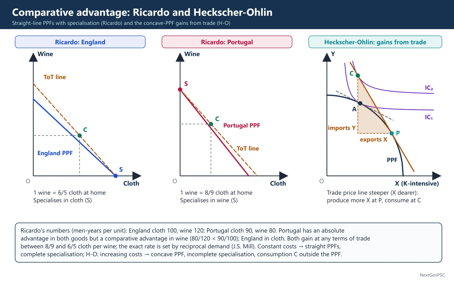
Ricardo's example: England needs 100 men-years for cloth and 120 for wine; Portugal needs 90 for cloth and 80 for wine; Portugal has an absolute advantage in both but a comparative advantage in wine (80/120 is less than 90/100), and England has a comparative advantage in cloth.
Domestic cost ratios: in Portugal 1 wine costs 8/9 cloth; in England 1 wine costs 6/5 cloth.
Terms of trade range: trade is mutually beneficial at any terms of trade between 8/9 and 6/5 cloth per unit of wine; the exact rate is set by reciprocal demand (J.S. Mill, Principles of Political Economy, 1848).
Gains: with specialisation and trade, both countries consume beyond their own PPF; world output of both goods rises.
Result: complete specialisation, because costs are constant.
Wages: the high-productivity country has higher wages; low wages in a poor country reflect low productivity, so trade with low-wage countries is not 'unfair' (a common confusion clarified by the model).
Evidence: G.D.A. MacDougall (1951) found that US exports relative to UK exports were higher in industries where US labour productivity was more than about twice the UK level, roughly matching the wage ratio; this supported Ricardo.
Criticisms: labour theory of value, constant costs and complete specialisation are unrealistic; it does not explain why productivity differs; it ignores demand, transport costs and adjustment costs.
3. Heckscher-Ohlin Model Step by Step
Sources: Eli Heckscher (1919, in Swedish) and Bertil Ohlin, Interregional and International Trade (1933); Ohlin received the Nobel Prize in 1977.
Assumptions: 2 countries, 2 goods, 2 factors (2×2×2); identical technology everywhere; different factor endowments; goods differ in factor intensity with no factor intensity reversal; constant returns to scale; identical homothetic tastes; perfect competition; factors mobile within, immobile between countries; no transport costs or trade barriers; incomplete specialisation.
H-O theorem: a country exports the commodity that uses its relatively abundant factor intensively and imports the commodity that uses its scarce factor intensively.
Mechanism: the abundant factor is cheaper before trade, so goods intensive in it are cheaper; trade raises their price and output.
Factor price equalisation (FPE): Paul Samuelson (1948, 1949), building on Lerner: under H-O assumptions, free trade equalises the absolute and relative returns to homogeneous factors across countries; trade in goods substitutes for factor mobility.
Stolper-Samuelson theorem (1941): a rise in the relative price of a good raises the real return to the factor used intensively in it and lowers the real return to the other factor; so protection helps the scarce factor (labour in rich countries) and free trade helps the abundant factor.
Rybczynski theorem (1955): at constant goods prices, an increase in the endowment of one factor raises the output of the good intensive in that factor more than proportionately and reduces the output of the other good.
Magnification effect: Ronald Jones (1965) showed that factor returns change by more than goods prices, and outputs by more than endowments.
Specific factors model: Jones (1971) and Samuelson: in the short run some factors are sector-specific, so trade benefits specific factors in export sectors and harms those in import-competing sectors, while the mobile factor's gain is ambiguous.
4. The Leontief Paradox
Test: Wassily Leontief (1953) used the 1947 US input-output table to compute the capital and labour needed to produce one million US dollars' worth of US exports and of import substitutes.
Finding: US import substitutes were about 30% more capital-intensive than US exports, though the US was thought to be the most capital-abundant country; this contradicted H-O.
Explanations: US labour is more productive (Leontief's own argument, about three times as efficient); human capital embodied in US exports (Kenen, Keesing); natural resources (Vanek) that are complementary to capital; factor intensity reversal (B.S. Minhas, 1962); US tariffs protecting labour-intensive industries (Kravis); demand bias towards capital-intensive goods.
Methodological critique: Edward Leamer (1980) showed that with trade imbalance the correct test compares the factor content of production and consumption; the US in 1947 was a net exporter of both capital and labour services, so it was revealed capital-abundant.
Indian study: R. Bharadwaj (1962) applied Leontief's method to India and found Indian exports to the US more capital-intensive than imports from it, another paradox.
Modern evidence: Trefler (1995) found 'missing trade': factor content of trade is much smaller than H-O predicts unless technology differences are allowed (H-O-V model, Vanek 1968).
5. Diagrams to Draw
Ricardian PPFs: draw cloth on the horizontal axis and wine on the vertical; draw straight-line PPFs for England and Portugal with different slopes; show specialisation at the axis intercepts and a terms of trade line between the two slopes; mark the consumption point outside each PPF.
H-O gains from trade: draw a concave PPF for a capital-abundant country with capital-intensive good X on the horizontal axis; autarky equilibrium A where a community indifference curve touches the PPF; with trade, the price line becomes steeper (X dearer, since its slope is Px/Py), production moves to P (more X), consumption to C on a higher indifference curve; the trade triangle shows exports of X and imports of Y.
Edgeworth box (FPE and Stolper-Samuelson): draw a box with labour on the horizontal side and capital on the vertical; draw the contract curve; show a movement along the curve towards more X raising K/L in both industries and the marginal product (wage) of labour falling or rising according to intensity.
Rybczynski line: draw two PPFs, the new one biased outward along the capital-intensive good's axis; at the same price slope the output of X rises and of Y falls.
6. Examples and Applications
India: India's labour abundance shows in exports of textiles, garments, leather and gems; its abundance of skilled English-speaking labour shows in software and IT-enabled services; its imports are capital- and resource-intensive (machinery, crude oil, electronics).
China: labour-intensive manufacturing exports after 1978 fit H-O; Stolper-Samuelson predicted pressure on low-skill wages in rich countries ('China shock' studies by Autor, Dorn and Hanson, 2013).
Dutch disease: a resource boom (Netherlands gas in the 1960s) expands the resource sector and shrinks manufacturing, a Rybczynski-type effect.
7. Using it in the Exam
10 marks: distinguish absolute and comparative advantage with Ricardo's numerical example.
15 marks: H-O theorem with assumptions, a PPF diagram and the FPE or Stolper-Samuelson corollary.
20 marks: Ricardo versus H-O, the Leontief paradox and its explanations (including Minhas and Leamer), and relevance to India's trade pattern.
Keywords: comparative advantage, opportunity cost, reciprocal demand, factor abundance, factor intensity, FPE, Stolper-Samuelson, Rybczynski, Leontief paradox, factor intensity reversal.
Quotation: Samuelson called comparative advantage the one proposition in the social sciences that is both true and non-trivial (paraphrased).
| Feature | Ricardo (1817) | Heckscher-Ohlin (1919, 1933) |
|---|---|---|
| Basis of trade | Differences in labour productivity (technology) | Differences in factor endowments |
| Factors | Labour only | Two factors (labour and capital) |
| Costs and PPF | Constant; straight-line PPF | Increasing; concave PPF |
| Specialisation | Complete | Incomplete |
| Effect on factor incomes | Not analysed (one factor) | FPE and Stolper-Samuelson: abundant factor gains |
| Empirical test | MacDougall (1951) broadly supportive | Leontief paradox (1953); Leamer (1980) reinterpretation |
Mains points
- Use Ricardo's original numbers (England 100/120, Portugal 90/80) and state the terms of trade range 8/9 to 6/5 cloth per wine.
- List H-O assumptions completely; marks are lost when no factor intensity reversal or identical technology is omitted.
- Present the three corollaries (FPE, Stolper-Samuelson, Rybczynski) in one line each with authors and years.
- For the Leontief paradox, give the finding (import substitutes about 30% more capital-intensive) and at least four explanations including Minhas (1962) and Leamer (1980).
- Relate to India: labour- and skill-intensive exports, capital and resource imports; mention Bharadwaj (1962).
- Common mistake: confusing absolute and comparative advantage, or saying H-O assumes different technologies.
Did you know?
- B.S. Minhas, the Indian economist who demonstrated factor intensity reversals in 1962 as a possible explanation of the Leontief paradox, later served as a member of India's Planning Commission.
Terms of Trade and Offer Curves
The terms of trade measure how many imports a country gets for its exports; the commonly used net barter (commodity) terms of trade is the ratio of export prices to import prices. Other concepts, such as income, single factoral and double factoral terms of trade, adjust for volumes and productivity. Offer curves (Marshall and Edgeworth) show how much of its export good a country will offer for imports at each price; their intersection fixes the equilibrium terms of trade and volume of trade. Growth can worsen a country's terms of trade so much that it becomes worse off (Bhagwati's immiserising growth, 1958).
In simple words
Terms of trade tell you how many foreign goods a country can buy with what it sells abroad.
If India sells tea and buys oil, and oil prices double while tea prices stay the same, India must export twice as much tea for the same oil: its terms of trade have worsened.
This matters because poorer countries exporting raw materials often face falling prices for their exports.
UPSC asks you to define the types of terms of trade, draw offer curves and discuss the Prebisch-Singer thesis.
1. Concepts of the Terms of Trade
Net barter (commodity) terms of trade (N): Taussig's term: N = (Px/Pm) × 100, where Px and Pm are export and import price (unit value) indices; a rise means each unit of exports buys more imports (improvement).
Gross barter terms of trade (G): F.W. Taussig, International Trade (1927): G = (Qm/Qx) × 100, the ratio of import volume to export volume; useful when there are unilateral transfers.
Income terms of trade (I): G.S. Dorrance (1948): I = (Px/Pm) × Qx, the capacity to import based on exports; it can improve even when N worsens if export volume rises enough.
Single factoral terms of trade (S): Jacob Viner (1937): S = N × Zx, where Zx is the productivity index in export industries; shows imports obtained per unit of domestic factors used in exports.
Double factoral terms of trade (D): D = N × (Zx/Zm), adjusting also for productivity in the foreign country's export industries; shows how many units of foreign factors exchange for one unit of domestic factors.
Real cost and utility terms of trade: Viner's further refinements adjusting for the disutility of producing exports and the utility of imports; not measurable in practice.
Interpretation caution: a fall in N due to productivity growth in exports (falling costs) need not mean welfare loss; the factoral terms may improve at the same time.
2. Offer Curves: Construction
Origin: the reciprocal demand idea of J.S. Mill was given diagrammatic form by Alfred Marshall (The Pure Theory of Foreign Trade, 1879) and F.Y. Edgeworth; J.E. Meade, A Geometry of International Trade (1952), derived them from trade indifference curves.
Definition: an offer curve shows, for each terms of trade, the quantity of exports a country is willing to give in exchange for a quantity of imports; it combines its demand for imports and its supply of exports.
Derivation: rotate the terms of trade line through the origin; at each price the country produces on its PPF and consumes where its highest indifference curve touches the price line; the trade triangle gives one point; joining such points gives the offer curve.
Shape: it starts at the origin, bends towards the import axis, and may bend backward when the demand for imports becomes inelastic (the country offers less exports even though it gets more imports).
Elasticity: the shape of the offer curve reflects the elasticity of demand for imports e: an elastic import demand (e above 1) gives an upward-sloping, elastic portion; unit elasticity gives a vertical (or horizontal) segment; inelastic demand gives the backward-bending portion.
3. Equilibrium and Comparative Statics
Equilibrium: where the two countries' offer curves intersect; the ray from the origin through the intersection is the equilibrium terms of trade; the coordinates give the volumes traded.
Stability: Marshall's stability condition for offer curves corresponds to the Marshall-Lerner condition: the sum of the import demand elasticities exceeds one.
Shift by growth or demand: if a country's demand for imports rises (or its export capacity grows), its offer curve shifts outward; the terms of trade worsen for it, and more so the less elastic the partner's offer curve.
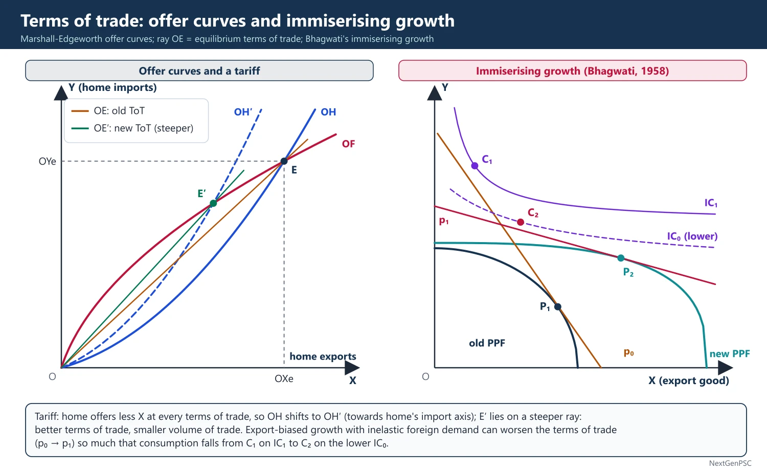
Effect of a tariff: a tariff shifts the imposing country's offer curve towards its own import axis (it offers less exports at each price); if the partner's offer curve is not perfectly elastic, the terms of trade improve for the imposing country; this is the basis of the optimal tariff t* = 1/(e* − 1), where e* is the elasticity of the foreign offer curve.
Metzler paradox: Lloyd Metzler (1949) showed that if the foreign offer curve is very inelastic, a tariff can improve the terms of trade so much that the domestic price of the import falls, hurting the protected industry.
Lerner symmetry: Abba Lerner (1936) showed that an import tariff and an export tax of the same rate have identical real effects.
4. Immiserising Growth
Source: Jagdish Bhagwati, 'Immiserizing Growth: A Geometrical Note' (Review of Economic Studies, 1958); earlier related ideas by Edgeworth (1894).
Result: growth biased towards the export sector can so worsen the terms of trade that the loss outweighs the gain from higher output, leaving the country worse off.
Conditions: growth strongly export-biased; the foreign demand for the country's exports price-inelastic; the country large enough in world markets to affect prices; and the country heavily dependent on trade.
Diagram logic: the PPF shifts out, biased towards the export good; the new terms of trade line is much flatter; the consumption point lies on a lower indifference curve than before growth.
Later extension: Harry Johnson (1967) showed that growth under a tariff (protected import-competing sector) can also be immiserising even for a small country.
5. Long-run Trends: Prebisch-Singer Thesis
Statement: Raúl Prebisch (The Economic Development of Latin America and Its Principal Problems, ECLA, 1950) and Hans Singer (American Economic Review, 1950) argued that the net barter terms of trade of primary producers tend to decline against manufactures.
Reasons: low income elasticity of demand for primary products (Engel's law); synthetic substitutes; productivity gains in manufacturing passed on as higher wages and profits in the industrial centre (strong unions, monopoly) but as lower prices in the periphery (surplus labour); and protection of agriculture in rich countries.
Policy conclusion: developing countries should industrialise, often through import substitution (influential in Latin America and India in the 1950s–70s).
Evidence: Grilli and Yang (1988) found a decline of roughly half a percentage point a year in non-fuel commodity prices relative to manufactures over 1900–86; others note quality improvement in manufactures and the 2000s commodity boom (debated).
Criticisms: Haberler and Viner questioned the data (base year, quality changes, transport costs in import prices); the thesis does not prove that trade is harmful, only that dependence on commodities is risky.
6. Diagrams to Draw
Offer curve equilibrium: draw the home country's export good X on the horizontal axis and import good Y on the vertical; draw home's offer curve OH bending towards the Y axis and the foreign offer curve OF bending towards the X axis; mark their intersection E; draw the ray OE as the terms of trade line; label OXe exports and OYe imports.
Tariff and offer curve: shift OH inward to OH′ (towards the Y axis, home's import axis); the new intersection E′ lies on a steeper ray, an improvement in home's terms of trade but a smaller volume of trade.
Immiserising growth: draw a PPF shifting out mostly along the export axis; draw the old price line tangent at the original production point and community indifference curve IC1; draw a much flatter new price line; show the new consumption point on IC0, below IC1.
Prebisch-Singer chart: plot time on the horizontal axis and the ratio of primary to manufactured goods prices on the vertical, showing a downward trend with fluctuations.
7. Examples and Applications
India: as a large importer of crude oil, India's net barter terms of trade improve when world oil prices fall (2014–16) and worsen when they rise (2022 after the Russia-Ukraine war), affecting the current account deficit.
Commodity exporters: Ghana (cocoa), Zambia (copper) and Venezuela (oil) suffered from terms-of-trade shocks, supporting the case for diversification.
Immiserising growth cases: often cited for coffee (Brazil) and jute (Bengal in the colonial period), where output growth met inelastic world demand.
8. Using it in the Exam
10 marks: define net barter, gross barter, income and factoral terms of trade with formulas.
15 marks: derive and draw offer curves, show equilibrium and the effect of a tariff.
20 marks: terms of trade concepts, offer curves, immiserising growth with conditions, and the Prebisch-Singer thesis with evidence and Indian relevance.
Keywords: net barter terms of trade, income terms of trade, factoral terms of trade, reciprocal demand, offer curve, optimal tariff, Metzler paradox, immiserising growth, secular decline.
Statement to quote: Bhagwati (1958) showed that export-biased growth facing inelastic foreign demand can reduce a country's welfare.
| Concept | Author | Formula | What it shows |
|---|---|---|---|
| Net barter (commodity) | Taussig | N = Px/Pm | Imports per unit of exports |
| Gross barter | Taussig (1927) | G = Qm/Qx | Volume of imports per volume of exports |
| Income | Dorrance (1948) | I = (Px/Pm) × Qx | Capacity to import from exports |
| Single factoral | Viner (1937) | S = N × Zx | Imports per unit of domestic factors in exports |
| Double factoral | Viner (1937) | D = N × Zx/Zm | Exchange of domestic for foreign factor units |
Mains points
- Give all terms of trade concepts with formulas and authors; a table is the fastest way to score.
- Explain why a fall in the net barter terms of trade need not reduce welfare (rising export volumes or productivity), using income and factoral terms.
- Draw the offer curve diagram carefully with the terms of trade ray; show the tariff effect and mention the optimal tariff formula.
- For immiserising growth, state all conditions and draw the diagram; credit Bhagwati (1958).
- Link Prebisch-Singer to India's import substitution strategy and to commodity-dependent economies today.
- Common mistake: drawing offer curves without labelling which good is exported by whom.
Did you know?
- Jagdish Bhagwati published his immiserising growth paper in 1958 at about the age of 24, and the term he coined is still standard in trade textbooks.
Product Cycle, New Trade Theory and Strategic Trade Policy
Classical theories explain trade by differences between countries; newer theories explain trade that H-O cannot. Posner's technological gap (1961) and Vernon's product life cycle (1966) show comparative advantage shifting from innovating to imitating countries as products mature. Linder (1961) explains trade in manufactures between countries of similar income. Krugman's new trade theory (1979, 1980) shows that economies of scale and product differentiation generate trade, including intra-industry trade, even between identical countries. Strategic trade policy (Brander and Spencer, 1985) shows that in oligopolistic industries a subsidy can shift profits to domestic firms.
In simple words
Old theories say countries trade because they are different; but Germany and France trade cars with each other, which old theories cannot explain.
Making cars is cheaper in huge factories, and buyers like variety, so each country specialises in a few models and they swap: Volkswagens for Renaults.
New products also start in rich countries and later move to cheaper places, like mobile phones now assembled in India.
UPSC asks about Vernon's product cycle, Krugman's new trade theory and whether governments should back 'national champions'.
1. Concepts and Definitions
Intra-industry trade: simultaneous export and import of products of the same industry (cars for cars); measured by the Grubel-Lloyd index (Herbert Grubel and Peter Lloyd, 1975): GL = 1 − |X − M|/(X + M), ranging from 0 (only inter-industry trade) to 1 (fully intra-industry).
Internal economies of scale: average cost falls as a firm's own output rises, leading to imperfect competition; external economies: cost falls as the industry's output in a location rises (Marshall's industrial districts), compatible with competition.
Product differentiation: varieties of a product that consumers see as imperfect substitutes (Chamberlin's monopolistic competition), giving 'love of variety' (Dixit-Stiglitz, 1977) or 'ideal variety' (Lancaster, 1980) preferences.
Strategic trade policy: government policy (subsidies, tariffs) that changes the strategic interaction between domestic and foreign oligopolists so as to shift rents to domestic firms.
2. Technological Gap and Product Life Cycle
Technological gap theory: Michael Posner (1961): a country that innovates enjoys a temporary export monopoly until foreign firms imitate; trade depends on the imitation lag (time for foreign producers to copy) minus the demand lag (time for foreign consumers to adopt the product); G.C. Hufbauer (1966) tested it for synthetic materials.
Product life cycle: Raymond Vernon, 'International Investment and International Trade in the Product Cycle' (Quarterly Journal of Economics, 1966).
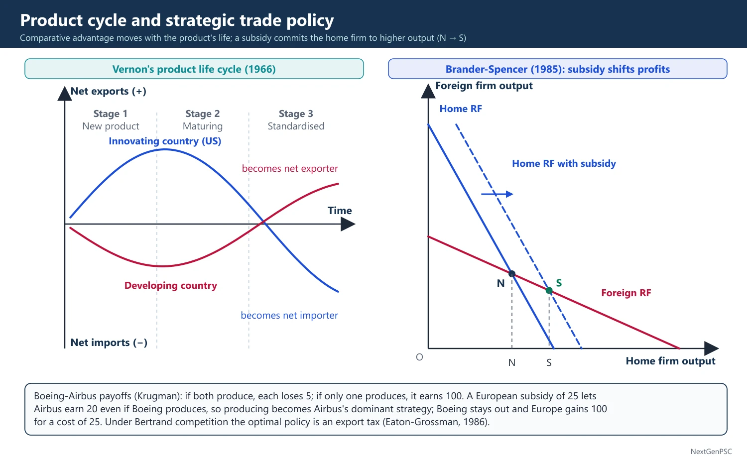
Stage 1, new product: produced in the innovating high-income country (the US in Vernon's case), close to rich consumers and skilled engineers; demand price-inelastic; small exports.
Stage 2, maturing product: methods become standard; demand grows abroad; the innovator exports and then sets up production in other developed countries to serve their markets (foreign direct investment).
Stage 3, standardised product: production is routine and price competition dominates; production moves to low-wage developing countries; the original innovator becomes a net importer.
Contribution: links trade with FDI and dynamic comparative advantage; explains the movement of radios, TVs, semiconductors and textiles from the US to Japan and then to East Asia.
Limitations: multinationals now innovate and launch globally at once; Vernon himself (1979) said the model had lost some of its power; it fits some industries (electronics) better than others (pharmaceuticals with patents).
3. Linder's Overlapping Demand Hypothesis
Source: Staffan Burenstam Linder, An Essay on Trade and Transformation (1961).
Idea: firms first produce for their home market, so a country exports manufactures for which there is a 'representative demand' at home; countries with similar per capita income have overlapping demand patterns and so trade more manufactures with each other.
Implication: trade in primary goods is explained by endowments (H-O), but trade in manufactures by demand similarity; this predicts heavy trade among rich countries, as observed.
Evidence: mixed; similar income countries do trade more, but distance (the gravity model of Tinbergen, 1962) explains much of the pattern.
4. Krugman's New Trade Theory
Sources: Paul Krugman, 'Increasing Returns, Monopolistic Competition, and International Trade' (Journal of International Economics, 1979) and 'Scale Economies, Product Differentiation, and the Pattern of Trade' (American Economic Review, 1980); Elhanan Helpman and Krugman, Market Structure and Foreign Trade (1985); Krugman received the Nobel Prize in 2008.
Model: firms produce differentiated varieties under internal economies of scale in monopolistic competition; consumers love variety; even two identical countries gain from trade because the integrated market supports more varieties and larger firms with lower average costs.
Gains from trade: more variety, lower prices through scale economies, and pro-competitive effects (lower markups); these gains exist without any comparative advantage.
Home market effect (1980): with transport costs, a country with a larger home demand for a good becomes its net exporter, because firms locate near the big market.
Pattern: inter-industry trade follows comparative advantage (H-O), intra-industry trade follows scale and variety; the more similar countries are in endowments, the larger the share of intra-industry trade (Helpman-Krugman).
Reciprocal dumping: James Brander (1981) and Brander-Krugman (1983): oligopolistic firms may sell the same good in each other's markets at prices below home prices, creating two-way trade in identical goods.
New new trade theory: Marc Melitz (Econometrica, 2003) introduced heterogeneous firms: only the most productive firms export; trade liberalisation raises average productivity by shifting market share to them.
Economic geography: Krugman, 'Increasing Returns and Economic Geography' (1991): scale economies and transport costs produce core-periphery patterns of industrial location.
5. Strategic Trade Policy
Brander-Spencer model: James Brander and Barbara Spencer, 'Export Subsidies and International Market Share Rivalry' (Journal of International Economics, 1985): a home and a foreign firm compete in a third market as Cournot duopolists; an export subsidy to the home firm commits it to higher output, the foreign firm cuts output, and home profits rise by more than the subsidy; national welfare rises at the foreign country's expense.
Boeing-Airbus illustration: Krugman's well-known payoff matrix: if both firms produce a new aircraft both lose (−5 each); if only one produces it earns 100; with a European subsidy of 25, Airbus earns 20 even if Boeing produces, so producing becomes Airbus's dominant strategy; Boeing stays out and Europe gains 100 for a cost of 25.
Sensitivity: Jonathan Eaton and Gene Grossman (1986) showed that under Bertrand (price) competition the optimal policy is an export tax, not a subsidy; the right policy depends on the form of competition, which governments rarely know.
Criticisms: retaliation leads to subsidy wars (a prisoners' dilemma); information requirements are huge; rent-seeking and lobbying; general-equilibrium effects (subsidising one sector draws resources from others, Dixit and Grossman, 1986); Krugman himself, 'Is Free Trade Passé?' (1987), concluded that free trade remains a good rule of thumb.
External economies argument: where an industry generates knowledge spillovers (semiconductors), support may be justified, but the spillovers must stay inside the country.
6. Diagrams to Draw
Product life cycle: draw time on the horizontal axis and net exports on the vertical for the innovating country (above the axis in stage 1–2, falling below in stage 3) and for a developing country (below in early stages, rising above in stage 3); label the three stages.
Krugman scale diagram: draw a falling average cost curve AC and a demand-related price line; show that a larger integrated market lets each firm move down AC to a lower cost and price, with more varieties.
Brander-Spencer reaction functions: draw home output on the horizontal and foreign output on the vertical; draw two downward-sloping Cournot reaction functions meeting at N (Nash equilibrium); a subsidy shifts the home reaction function right; the new equilibrium S is a Stackelberg-type point with higher home and lower foreign output.
Payoff matrix: draw a 2×2 table for Boeing and Airbus (produce/not produce) with and without the subsidy.
7. Examples and Applications
India: mobile phone assembly moved to India through Production Linked Incentive (PLI) schemes introduced from 2020 (later covering 14 sectors), a mix of product cycle relocation and strategic industrial policy; the India Semiconductor Mission (approved December 2021 with an outlay of ₹76,000 crore) supports fabs and assembly units.
Intra-industry trade in India: rising in automobiles and auto components, chemicals and pharmaceuticals.
World: the Boeing-Airbus subsidy disputes at the WTO (from 2004) ended in a five-year truce between the US and EU in June 2021; the US CHIPS and Science Act (2022) is strategic support to semiconductors.
East Asia: Japan, Korea and Taiwan moved up the product cycle from textiles to electronics and semiconductors (the 'flying geese' pattern described by Kaname Akamatsu).
8. Using it in the Exam
10 marks: stages of Vernon's product cycle with an example, or the Grubel-Lloyd index with interpretation.
15 marks: Krugman's model of trade under increasing returns and monopolistic competition, and why identical countries trade.
20 marks: new trade theory versus H-O, strategic trade policy (Brander-Spencer, Eaton-Grossman), criticisms and India's PLI and semiconductor policy as applications.
Keywords: imitation lag, product life cycle, representative demand, intra-industry trade, economies of scale, love of variety, home market effect, rent shifting, reaction function.
Statement to quote: Krugman (1979) showed that trade need not be a result of international differences in technology or factor endowments; it can be driven by economies of scale.
| Theory | Author and year | Basis of trade | Market structure | Trade explained |
|---|---|---|---|---|
| Comparative cost | Ricardo (1817) | Productivity differences | Perfect competition | Inter-industry |
| Factor endowment | Heckscher-Ohlin (1919, 1933) | Endowment differences | Perfect competition | Inter-industry |
| Technological gap / product cycle | Posner (1961); Vernon (1966) | Innovation and imitation lags | Temporary monopoly | Shifting comparative advantage; FDI |
| Overlapping demand | Linder (1961) | Similar income and tastes | Not specified | Manufactures among similar countries |
| New trade theory | Krugman (1979, 1980) | Scale economies, variety | Monopolistic competition | Intra-industry |
| Strategic trade | Brander-Spencer (1985) | Rent shifting by policy | Oligopoly | Trade in oligopolistic industries |
Mains points
- Describe the three stages of Vernon's cycle with locations of production and trade flows at each stage, and add a diagram.
- Explain why new trade theory was needed: the large share of intra-industry trade among similar rich countries, which H-O cannot explain.
- Give the Grubel-Lloyd index formula; it is an easy quantitative point.
- For strategic trade policy, use the Brander-Spencer reaction function diagram or the Boeing-Airbus matrix, then the Eaton-Grossman reversal and the retaliation critique.
- Apply to India: PLI schemes, the semiconductor mission, mobile phone exports, and the WTO compatibility of subsidies.
- Common mistake: treating strategic trade theory as a general case for protection; it applies only to oligopolistic industries with rents.
Did you know?
- Krugman has recalled that the key insight behind his 1979 paper came in early 1978, when he saw that the Dixit-Stiglitz (1977) model of monopolistic competition could be applied to international trade.
Trade as an Engine of Growth and Theories of Underdevelopment
D.H. Robertson (1938) and Ragnar Nurkse (1959) described 19th-century trade as an engine of growth that carried Britain's growth to the regions of recent settlement, but Nurkse argued the engine had weakened for 20th-century primary exporters. Irving Kravis (1970) replied that trade is a handmaiden, not an engine: domestic factors decide growth. Optimists stress dynamic gains (scale, technology, competition, vent for surplus) and the East Asian export-led success; pessimists, from Prebisch-Singer and Myrdal's backwash effects to dependency and unequal exchange theories, argue that trade on existing terms can keep poor countries underdeveloped.
In simple words
Can selling to the world make a poor country rich? South Korea grew rich by exporting; many African countries exporting raw materials stayed poor.
Trade is like a highway: it helps a town grow only if the town has goods, skills and roads to use it; otherwise traffic just passes through.
Economists debate whether trade drives growth (an engine) or only helps it (a handmaiden), and why some trading countries remain underdeveloped.
UPSC asks you to evaluate this debate with theories and examples such as East Asia and India after 1991.
1. Concepts and Definitions
Engine of growth: D.H. Robertson ('The Future of International Trade', Economic Journal, 1938) described 19th-century trade as an engine of growth; Ragnar Nurkse, Patterns of Trade and Development (Wicksell Lectures, 1959), developed the idea: rising British demand for food and raw materials transmitted growth to the regions of recent settlement (the US, Canada, Australia, New Zealand, Argentina, South Africa).
Handmaiden of growth: Irving Kravis, 'Trade as a Handmaiden of Growth' (Economic Journal, 1970): successful 19th-century countries grew mainly because of domestic factors (land, institutions, immigration, capital); trade supported but did not cause growth.
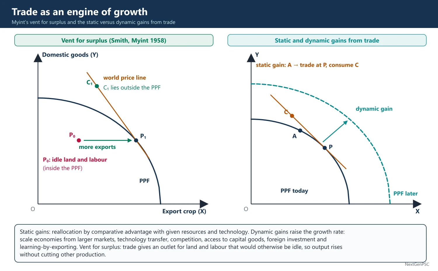
Static gains: gains from reallocating resources according to comparative advantage at given resources and technology.
Dynamic gains: gains that raise the growth rate: economies of scale from larger markets, technology transfer, competition and efficiency, access to capital goods, foreign investment and learning-by-exporting.
Vent for surplus: Adam Smith's idea, developed by Hla Myint ('The Classical Theory of International Trade and the Underdeveloped Countries', Economic Journal, 1958): trade gives an outlet for surplus land and labour that would otherwise be idle, so output rises without cutting other production.
2. Nurkse's Argument: Why the Engine Weakened
19th century: trade carried growth because Britain's demand for primary products rose rapidly and capital and labour migrated with it.
20th century slowdown in demand for primary products: (i) shift of industrial output to industries with low raw material content (engineering, chemicals); (ii) rising share of services in rich-country GDP; (iii) low income elasticity of demand for food (Engel's law); (iv) agricultural protection in industrial countries; (v) economy in raw material use and synthetic substitutes (rubber, fibres).
Conclusion: primary exporting LDCs could not rely on trade to grow; Nurkse favoured balanced growth with domestic markets, while accepting gains from trade.
Haberler's reply: Gottfried Haberler, International Trade and Economic Development (Cairo lectures, 1959), stressed that trade provides capital goods, technology, competition and ideas, and that pessimism about export demand was exaggerated.
Lewis on the engine: W. Arthur Lewis, 'The Slowing Down of the Engine of Growth' (Nobel lecture, 1979, published 1980), linked the growth of developing countries' exports to growth in the industrial countries and warned that a slowdown in the latter would slow the former unless developing countries traded more among themselves.
3. Arguments that Trade Promotes Growth
Export-led growth: exports relax the foreign exchange constraint (two-gap model of Chenery and Strout, 1966), finance imports of capital goods and allow scale economies beyond a small home market.
Learning and technology: exporters learn from foreign buyers; imports embody technology; FDI brings management and spillovers (endogenous growth models of Grossman and Helpman, 1991).
Competition: openness disciplines monopolies and rent-seeking (Krueger, 1974; Bhagwati).
Evidence: the East Asian economies (Japan, South Korea, Taiwan, Hong Kong, Singapore, later China) grew rapidly with outward orientation (World Bank, The East Asian Miracle, 1993); cross-country studies such as Sachs and Warner (1995) and Frankel and Romer (1999) found openness associated with faster growth.
Critique of the evidence: Rodríguez and Rodrik (2000) argued that openness measures were flawed and mixed with other policies; Amsden and Wade showed East Asian states used industrial policy and selective protection, not laissez-faire (debated).
4. Theories of Underdevelopment in an Open Economy
Prebisch-Singer (1950): secular decline in the terms of trade of primary exporters and asymmetric distribution of productivity gains between centre and periphery.
Singer on enclaves (1950): foreign investment in export enclaves (mines, plantations) created few linkages with the rest of the economy; its benefits went abroad.
Myrdal's cumulative causation: Gunnar Myrdal, Economic Theory and Under-developed Regions (1957): trade and factor movements produce backwash effects (flows of capital, skilled labour and trade advantage towards already rich regions) stronger than spread effects (demand for the poor region's products, diffusion of technology); free markets widen inequality between and within countries.
Dependency theory: Paul Baran, The Political Economy of Growth (1957); Andre Gunder Frank, 'The Development of Underdevelopment' (1966): the periphery's surplus is extracted by the metropolis, so underdevelopment is a product of integration into world capitalism, not of isolation.
Unequal exchange: Arghiri Emmanuel, Unequal Exchange (1969 in French, 1972 in English): with international capital mobility but immobile labour, large wage differences mean that poor countries exchange more labour-hours for fewer; Samir Amin extended it.
World-systems theory: Immanuel Wallerstein (1974) analysed core, semi-periphery and periphery in a single world economy.
Lewis on tropical trade: W.A. Lewis (1969, Aspects of Tropical Trade) argued that the factoral terms of trade of tropical exports were set by low productivity in subsistence food production, keeping export wages low.
Resource curse and Dutch disease: resource booms appreciate the real exchange rate, shrink manufacturing and encourage rent-seeking (Sachs and Warner, 1995).
Export instability: fluctuating commodity earnings disrupt investment (Coppock); A.I. MacBean (1966) found the harmful effects smaller than claimed (debated).
Indian precursor: Dadabhai Naoroji's drain theory, Poverty and Un-British Rule in India (1901), argued that colonial trade and remittances drained India's surplus.
5. Assessment
Synthesis: trade raises growth when complementary conditions exist (human capital, infrastructure, macro stability, institutions, a diversified export base); without them, gains are small and benefits may leak abroad.
Policy implication: outward orientation combined with active capability-building (education, infrastructure, export promotion) rather than either autarky or passive laissez-faire.
Current debate: rising protectionism, global value chains and slowing world trade growth after 2008 ('slowbalisation') have revived questions about whether export-led growth can be repeated (Rodrik's 'premature deindustrialisation', 2016).
6. Diagrams to Draw
Vent for surplus: draw a PPF and a production point P0 inside it (idle resources); with trade, production moves to P1 on the PPF (more exports) and consumption to C1 outside the PPF without reducing domestic goods.
Static versus dynamic gains: draw a PPF with the static gain (move along PPF and trade) and then an outward shift of the PPF over time showing dynamic gains.
Myrdal's cumulative causation chart: draw two circles, rich region and poor region; arrows of capital, skilled labour and trade flowing to the rich region (backwash) and thinner arrows of demand and technology flowing to the poor region (spread).
Terms of trade trend: plot primary product prices relative to manufactures over time with a falling trend line.
7. Examples and Applications
India: from 1950 to 1990 export pessimism (Mahalanobis strategy) led to inward-looking import substitution; Bhagwati and Desai, India: Planning for Industrialization (1970), criticised its inefficiency; after 1991 opening, exports of goods and services grew strongly, reaching about 825 billion US dollars in 2024–25 (Ministry of Commerce), led by services such as software.
East Asia: South Korea's exports rose from a very small share of GDP in the early 1960s to a major share by the 1980s with rapid industrial upgrading.
Africa and Latin America: commodity dependence and terms-of-trade shocks (Zambia copper, Venezuela oil) illustrate pessimist arguments.
8. Using it in the Exam
10 marks: distinguish engine and handmaiden views with authors and years.
15 marks: Nurkse's reasons for the weakening engine and Haberler's or Kravis's replies.
20 marks: trade as engine of growth versus theories of underdevelopment (Prebisch-Singer, Myrdal, dependency, unequal exchange), with East Asia and India as evidence and a balanced conclusion.
Keywords: engine of growth, handmaiden, dynamic gains, vent for surplus, export pessimism, backwash and spread effects, centre-periphery, dependency, unequal exchange, export-led growth.
Quotation: Kravis (1970) argued that trade has been a handmaiden rather than an engine of growth (paraphrased).
| View | Key authors | Main claim | Evidence cited |
|---|---|---|---|
| Engine of growth | Robertson (1938), Nurkse (1959) | Trade transmitted growth in the 19th century | Regions of recent settlement |
| Handmaiden | Kravis (1970) | Domestic factors cause growth; trade helps | 19th-century success stories |
| Dynamic gains / export-led | Haberler (1959), Myint (1958), Krueger, Bhagwati | Openness raises efficiency, scale, technology | East Asia; India after 1991 |
| Terms-of-trade pessimism | Prebisch, Singer (1950) | Primary exporters lose from trade | Long-run decline in commodity prices |
| Cumulative causation | Myrdal (1957) | Backwash exceeds spread effects | Regional and international divergence |
| Dependency / unequal exchange | Baran (1957), Frank (1966), Emmanuel (1969) | Integration causes underdevelopment | Latin America, colonial economies |
Mains points
- Frame the answer as a debate: engine (Robertson, Nurkse for the 19th century) versus handmaiden (Kravis), then optimists versus pessimists for LDCs.
- List Nurkse's five reasons for the weakening of the engine; examiners expect them.
- Distinguish static and dynamic gains and include vent for surplus (Myint) as a gain specific to underdeveloped countries.
- Present underdevelopment theories with authors and works: Prebisch-Singer, Singer's enclaves, Myrdal's backwash, Frank, Emmanuel, Wallerstein.
- Use evidence on both sides: East Asia and India after 1991 versus commodity-dependent economies; mention Rodríguez-Rodrik's critique.
- Conclude that trade is a powerful handmaiden that needs domestic capabilities; avoid one-sided conclusions.
Did you know?
- Andre Gunder Frank's phrase 'the development of underdevelopment' (1966) became a slogan of dependency theory, turning the usual idea upside down: poverty was produced by integration into the world economy, not by isolation from it.
UPSC Previous Year Questions: Theories of International Trade
From 2014 to 2026 UPSC asked 26 question parts (350 marks) from Theories of International Trade. Comparative advantage, Heckscher-Ohlin and its theorems (9 parts) and new trade theory, product cycle and intra-industry trade (9 parts) dominate, followed by offer curves and terms of trade, immiserising growth and trade as an engine of growth. Every question below has a model answer written to the UPSC word limit.
In simple words
Read the question and spend five minutes writing your own outline: the theorem and who gave it, its assumptions, the diagram and a conclusion.
Then read the model answer and tick what you missed: the exact statement of the theorem, the condition, the diagram (PPF, offer curves) or the empirical test.
Rewrite one answer a day within the word limit (10 marks about 150 words, 15 marks about 200, 20 marks about 250) and practise the diagrams until they are quick and neat.
1. Comparative Advantage: Ricardo and Heckscher-Ohlin
Example 1 (UPSC 2025, 10 marks): State Heckscher-Ohlin theory. Explain the Leontief Paradox in this context.
Paper and question: Paper I, Q5(c)
Approach: State the H-O theorem with its assumptions, then explain Leontief's test and finding and the main explanations of the paradox.
Heckscher-Ohlin theorem (Heckscher, 1919; Ohlin, 1933): a country exports the good that uses intensively its relatively abundant factor and imports the good that uses intensively its scarce factor. It assumes two countries, two goods and two factors, identical technology and tastes, constant returns, perfect competition, and no factor intensity reversal.
Leontief Paradox: Wassily Leontief (1953), using the US input-output table for 1947, compared the capital per worker needed to produce US exports with that needed for import substitutes. Although the US was the most capital-abundant country, its import-competing goods were about 30% more capital-intensive than its exports, the opposite of the H-O prediction.
Explanations: (i) US labour was more productive (Leontief himself suggested about three times), so the US was really labour-abundant in efficiency units; (ii) human capital: US exports were skill-intensive (Kenen, Keesing); (iii) natural resources omitted from the two-factor test; (iv) US tariffs protected labour-intensive industries; (v) factor intensity reversal (Minhas, 1962); (vi) demand biased towards capital-intensive goods.
Later multi-factor tests (Leamer, 1980) reconciled much of the paradox.
Example 2 (UPSC 2024, 15 marks): By using Stolper-Samuelson theorem, discuss the possible effects of free trade on income inequalities in developing countries.
Paper and question: Paper I, Q6(b)
Approach: State the Stolper-Samuelson theorem and its prediction for labour-abundant developing countries, then examine the evidence and the reasons why liberalisation has often raised inequality, and conclude.
Stolper-Samuelson theorem (1941): in the 2×2 H-O model, a rise in the relative price of a good raises the real return of the factor used intensively in producing it and lowers the real return of the other factor, with a magnification effect (the factor price changes more than proportionately).
Prediction for developing countries: these countries are abundant in unskilled labour. Free trade raises the relative price of their labour-intensive exports (textiles, garments, assembly), so real wages of unskilled workers rise and returns to capital and skill fall. Inequality between labour and capital, and between unskilled and skilled workers, should therefore fall.
Evidence: after liberalisation in Mexico, Colombia, Brazil and India, wage inequality often rose (Goldberg and Pavcnik, 2007). Reasons: (i) before reform the most protected sectors were often unskilled-labour-intensive, so tariff cuts lowered their relative prices; (ii) outsourcing within global value chains moves tasks that are skill-intensive for the developing country (Feenstra and Hanson); (iii) trade brings skill-biased technology; (iv) many factors and imperfect mobility between sectors and regions; (v) large informal sectors and entry of China and other low-wage exporters, which kept prices of labour-intensive goods low.
Hence Stolper-Samuelson implies that free trade should reduce inequality in labour-abundant countries, but in practice the effect depends on the pattern of protection, technology and labour mobility; complementary policies such as education, skills and social protection are needed.
Example 3 (UPSC 2023, 10 marks): "Factor intensity reversal is incompatible with Heckscher-Ohlin model." Examine this statement.
Paper and question: Paper I, Q5(a)
Approach: Define factor intensity reversal, show with isoquants why it arises (different elasticities of substitution), explain why it invalidates the H-O theorem for one country, and cite Minhas and Leontief.
Factor intensity reversal occurs when a good is capital-intensive at one set of factor prices and labour-intensive at another. It arises when the elasticities of substitution between capital and labour differ between the two industries, so their isoquants cross twice.
Diagram: unit isoquants of X and Y in (L, K) space crossing at two points; at a low wage-rental ratio X is labour-intensive, at a high ratio X is capital-intensive.
The statement is correct. H-O requires that goods can be ranked by factor intensity at all factor prices. With a reversal, suppose X is labour-intensive in labour-abundant India (low w/r) but capital-intensive in the capital-abundant US (high w/r). H-O predicts that India exports X and that the US exports X too, which is impossible: both cannot export the same good to each other. So the theorem fails for one country, and factor-price equalisation also breaks down.
Empirically, Minhas (1962) found frequent reversals using CES production functions, but Leontief (1964) showed that most disappeared when a few natural-resource industries were excluded; reversals are therefore possible but not common.
Example 4 (UPSC 2022, 10 marks): Discuss the Factor Endowment theory of trade in terms of 'abundance in factor prices' and 'factor abundance'.
Paper and question: Paper I, Q1(d)
Approach: Distinguish the price definition and the physical definition of factor abundance, show how each relates to the H-O theorem (demand matters only under the physical definition), with a diagram.
The Heckscher-Ohlin factor endowment theory explains trade by differences in relative factor abundance, defined in two ways.
Price definition (abundance in factor prices): a country is capital-abundant if its autarky ratio of the price of capital to the price of labour (r/w) is lower than abroad. Since relative factor prices reflect both supply and demand, the capital-abundant country's capital-intensive good is relatively cheap, and the H-O theorem always holds under this definition (given no factor-intensity reversal).
Physical definition (factor abundance): a country is capital-abundant if its ratio of total capital to total labour (K/L) is higher. This considers only supply. Its PPF is biased towards the capital-intensive good, but if domestic demand is strongly biased towards that good, its relative price may not be lower, and the country could export the labour-intensive good; H-O then needs identical, homothetic tastes to hold.
Diagram: a PPF skewed towards the capital-intensive good X; with identical tastes the autarky price of X is lower; with a strong demand bias towards X the indifference curve can make X relatively dearer.
Hence the price definition makes H-O tautologically valid, while the physical definition makes it testable, as in Leontief's test.
Example 5 (UPSC 2022, 15 marks): Examine whether in Ricardian model, the theory of comparative advantage actually becomes a doctrine of comparative costs.
Paper and question: Paper I, Q7(a)
Approach: Explain Ricardo's comparative advantage based on relative labour costs, show how with money wages it becomes a matter of comparative (real) costs translated into money prices (Taussig), then note the limits (labour theory of value, demand) and later reformulations.
In Ricardo's model (Principles, 1817) labour is the only factor and the value of a good equals the labour embodied in it. A country has a comparative advantage in the good whose relative labour cost (a₁/a₂) is lower than abroad; in his example Portugal needed less labour for both wine and cloth, but its advantage was greater in wine, so it exported wine.
Yes, the theory is essentially a doctrine of comparative costs: the advantage is defined entirely by comparing ratios of real labour costs.
Money prices: traders respond to money prices. Taussig showed that with money wages and an exchange rate, comparative cost differences become absolute differences in money prices: Portugal's higher wage (justified by its higher productivity) must lie within the range set by its productivity advantages, so wine is cheaper in Portugal and cloth cheaper in England in money terms. The wage ratio must lie between the productivity ratios of the two goods for trade to be two-way.
Limits: the doctrine rests on the labour theory of value and a single factor; it says nothing about demand, so J.S. Mill's reciprocal demand was needed to fix the terms of trade. Haberler (1936) restated it in terms of opportunity costs, freeing it from the labour theory.
So in the Ricardian model comparative advantage is indeed a doctrine of comparative real costs, which money prices merely reflect.
Example 6 (UPSC 2018, 15 marks): Explain, with the help of diagram, how Haberler's theory of opportunity cost is an improvement over the comparative cost theory of Ricardo.
Paper and question: Paper I, Q6(a)
Approach: Explain Haberler's opportunity-cost restatement (1936), show it with PPF diagrams (constant and increasing costs, trade triangle), and list how it improves on Ricardo.
Ricardo's comparative cost theory relied on the labour theory of value: costs were measured in labour hours, labour was homogeneous and the only factor. Gottfried Haberler (The Theory of International Trade, 1936) restated comparative advantage in terms of opportunity cost: the cost of a unit of X is the amount of Y that must be given up to produce it.
Explanation with diagram: each country's production possibility frontier (PPF) with X and Y on the axes. With constant opportunity costs the PPF is a straight line whose slope is the autarky price ratio; the country with the flatter slope has a comparative advantage in X. With trade at international terms of trade between the two slopes, each specialises completely and consumes at a point outside its PPF on the trade line. With increasing costs the PPF is concave; production moves along it to the point where its slope equals the terms of trade, specialisation is incomplete, and the trade triangle shows exports and imports; consumption reaches a higher indifference curve.
Improvements: (i) it frees the theory from the labour theory of value and allows many factors; (ii) it can handle increasing costs, explaining incomplete specialisation; (iii) combined with community indifference curves it shows gains from trade in welfare terms.
Its weakness is that it still does not explain why opportunity costs differ, which Heckscher-Ohlin later did.
Example 7 (UPSC 2016, 15 marks): "Technical progress in capital-intensive sector almost invariably reduces the real wage rate and increases the real return to capital. Technical progress in labour-intensive sector will lead to increase in real wage rate and decrease in the real return to capital." Explain.
Paper and question: Paper I, Q6(b)
Approach: Use the 2×2 H-O model with given goods prices (small economy): explain via the zero-profit conditions (Findlay-Grubert) how neutral technical progress in one sector changes factor rewards, with the Lerner-Pearce or unit-cost diagram, and the role of bias.
This is the result of Findlay and Grubert (1959), derived in the two-good, two-factor model with given commodity prices (a small open economy) and perfect competition, where price equals unit cost in each sector.
Mechanism: technical progress in the capital-intensive sector lowers its unit cost, so at the given price it earns profits and expands, drawing resources from the labour-intensive sector. The capital-intensive sector demands relatively more capital and less labour than the labour-intensive sector releases, so the rental on capital rises and the wage falls until zero profits are restored in both sectors. As in the Stolper-Samuelson theorem, the effect is magnified: the factor used intensively in the progressing sector gains in real terms, the other loses. Symmetrically, progress in the labour-intensive sector raises the real wage and lowers the real return to capital.
Diagram: unit-cost curves in (w, r) space for the two sectors (the price-equals-cost loci); progress in sector X shifts its curve outwards; the intersection moves to a higher r and lower w when X is capital-intensive.
'Almost invariably' because the result holds for neutral and for labour-saving progress; if progress in the capital-intensive sector is strongly capital-saving, it reduces that sector's demand for capital and the outcome can be reversed. If goods prices change (a large country), the terms-of-trade effect also matters.
The result explains why productivity growth in sectors such as electronics benefits capital, while growth in labour-intensive sectors benefits workers.
Example 8 (UPSC 2014, 10 marks): What is meant by 'factor abundance'? How does it affect the shape of the production frontier of a nation?
Paper and question: Paper I, Q5(a)
Approach: Define factor abundance (physical and price definitions) and show how it biases the shape of the PPF towards the good intensive in the abundant factor, with a diagram.
Factor abundance in the Heckscher-Ohlin theory compares relative factor endowments of countries. In physical terms, a country is capital-abundant if its ratio of capital to labour (K/L) exceeds that of its partner; in price terms, if its autarky ratio of rental to wage (r/w) is lower.
Effect on the PPF: because goods differ in factor intensity, a country can produce relatively more of the good that uses its abundant factor intensively. Its PPF is therefore stretched, or biased, towards that good. A capital-abundant country such as the US has a PPF skewed towards capital-intensive machinery; a labour-abundant country such as India has one skewed towards labour-intensive textiles. By the Rybczynski theorem (1955), a larger endowment of a factor raises the output of the good using it intensively and, at constant prices, reduces the output of the other good.
Diagram: two concave PPFs on the same axes (X capital-intensive on the horizontal, Y labour-intensive on the vertical): the capital-abundant country's PPF extends further along the X axis, the labour-abundant country's further along the Y axis.
With identical tastes, the abundant factor's good is relatively cheaper in autarky, which gives the comparative advantage predicted by H-O.
Example 9 (UPSC 2014, 10 marks): Explain the conditions under which complete specialisation will be possible for two nations in case of comparative advantage. Suppose productivity per unit of labour for two nations, India and UK, is given as under:
India / UK
Wheat (kg)/manhour: 06 / 03
Cloth (yard)/manhour: 04 / 02
Will mutually beneficial trade be possible for the two nations? If yes, explain whether specialisation shall be complete or not.
Paper and question: Paper I, Q6(c)
Approach: State the conditions for complete specialisation, then compare opportunity-cost ratios for India and the UK step by step and conclude whether trade is mutually beneficial.
Conditions for complete specialisation: in the Ricardian model with constant opportunity costs (straight-line PPFs), each country specialises completely when the international terms of trade lie strictly between the two countries' autarky price ratios, and neither country is so large relative to the other that the small partner cannot meet its demand. With increasing costs (concave PPFs), specialisation is normally incomplete.
Step 1: India: 6 kg wheat or 4 yards cloth per man-hour, so 1 yard of cloth costs 6/4 = 1.5 kg of wheat (1 kg wheat costs 0.67 yard).
Step 2: UK: 3 kg wheat or 2 yards cloth per man-hour, so 1 yard of cloth costs 3/2 = 1.5 kg of wheat (1 kg wheat costs 0.67 yard).
Step 3: India has an absolute advantage in both goods (twice the UK's productivity in each), but the opportunity-cost ratios are identical (1.5 = 1.5), so neither country has a comparative advantage.
In words: mutually beneficial trade is not possible. At any terms of trade other than 1.5 kg wheat per yard, one country would lose; at exactly 1.5 neither gains. Hence there is no basis for specialisation, complete or partial. As Ricardo showed, it is differences in comparative, not absolute, costs that create gains from trade.
2. Terms of Trade and Offer Curves
Example 10 (UPSC 2025, 10 marks): Define offer curve and explain its slope.
Paper and question: Paper I, Q5(a)
Approach: Define the offer curve (Marshall-Edgeworth), explain how it is derived and what its slope shows (terms of trade along rays; elastic, unit-elastic and inelastic segments), with a diagram.
An offer curve (reciprocal demand curve), developed by Alfred Marshall and F.Y. Edgeworth from J.S. Mill's reciprocal demand, shows the quantities of exports a country is willing to offer for different quantities of imports at all possible terms of trade. It combines its demand for imports and its supply of exports, and is derived from its PPF and indifference curves (trade triangles) as the terms of trade change.
Slope: the terms of trade at any point are shown by the slope of the ray from the origin to that point. As the terms of trade improve (steeper ray for the country), it offers more exports for more imports, so the curve bends towards its import axis. Along its rising part the country's demand for imports is elastic; where it becomes vertical (or horizontal) demand is unit-elastic; and if it bends backwards, demand is inelastic, the country offering fewer exports for more imports.
Diagram: country A's exports X on the horizontal axis and imports Y on the vertical; A's offer curve rises from the origin, bending towards the Y axis; rays from the origin show different terms of trade.
The intersection with the partner's offer curve fixes the equilibrium terms of trade.
Example 11 (UPSC 2024, 10 marks): Explain how the equilibrium terms of trade are determined by using offer curves of the trading partners.
Paper and question: Paper I, Q5(e)
Approach: Draw both offer curves, show that their intersection gives the equilibrium terms of trade and trade volumes, explain stability and the effect of a shift (e.g. a tariff or increased demand).
The offer curve of each country (Marshall, Edgeworth) shows how much of its export good it will give for various amounts of its import good at each terms of trade. Home exports X and imports Y; Foreign exports Y and imports X.
Diagram: X on the horizontal axis and Y on the vertical; Home's offer curve OH rises from the origin bending towards the Y axis; Foreign's offer curve OF rises bending towards the X axis; they intersect at E; the ray OE gives the equilibrium terms of trade, and the coordinates of E give Home's exports of X and imports of Y (equal to Foreign's imports and exports).
At any other terms of trade, Home's offer of X does not match Foreign's demand for X, so there is excess demand or supply and the terms of trade adjust until the two offers match at E, where trade is balanced. The equilibrium is stable when the sum of the import demand elasticities exceeds one (the Marshall-Lerner condition in real terms).
If Home's demand for Y rises or it imposes a tariff, its offer curve shifts; a tariff shifts OH towards its import axis (less X offered for each quantity of Y) and, for a large country, improves its terms of trade, while the volume of trade falls. The more elastic the partner's offer curve, the less the terms of trade change.
Example 12 (UPSC 2022, 15 marks): Illustrate Jagdish Bhagwati's doctrine of 'Immiserising Growth'.
Paper and question: Paper I, Q7(c)
Approach: Define immiserising growth (Bhagwati, 1958), state its conditions, illustrate with the PPF and terms-of-trade diagram, and give examples and policy implications.
Jagdish Bhagwati ('Immiserizing Growth: A Geometrical Note', 1958) showed that economic growth can make a country worse off: the welfare loss from a deterioration in its terms of trade can exceed the welfare gain from the growth itself.
Conditions: (i) growth is strongly export-biased, raising the supply of the export good much more than domestic demand for it; (ii) the country is large enough in world markets for its extra exports to lower world prices; (iii) foreign demand for its exports is price-inelastic; (iv) the country depends heavily on trade, so the terms-of-trade loss weighs heavily. Growth is immiserising when this loss exceeds the gain from higher output valued at the old prices.
Diagram: the PPF shifts outwards, biased towards the export good X; before growth the economy produces at P₁ and consumes at C₁ on indifference curve IC₁ with terms of trade line T₁; after growth, the terms of trade worsen to a flatter line T₂; production moves to P₂ on the new PPF, and the consumption point C₂ on T₂ lies on a lower indifference curve IC₂.
Illustrations: primary-product exporters whose expanded output of coffee, cocoa or jute depressed world prices; it is also linked to the Prebisch-Singer thesis. Harry Johnson (1967) showed a related result: capital accumulation in a tariff-protected import-competing sector can also reduce welfare.
Policy: an optimal export tax or production restraint, diversification away from inelastic exports, and stimulating domestic demand prevent immiserisation. Bhagwati (1968) generalised the idea: growth in the presence of distortions such as protection can also be immiserising.
Example 13 (UPSC 2014, 20 marks): Distinguish between single and double factor terms of trade. Explain how far terms of trade of a developing economy would change with technological advancement and economic growth.
Paper and question: Paper I, Q7(b)
Approach: Define single factoral and double factoral terms of trade with formulas (and their relation to net barter terms), then analyse how technical progress and growth (export-biased, import-biased, neutral) affect a developing country's terms of trade, with Prebisch-Singer.
The net barter terms of trade are N = Px/Pm, the ratio of export to import price indices. Factoral terms (Viner) adjust it for productivity.
Single factoral terms of trade: S = (Px/Pm) × Zx, where Zx is the productivity index of the country's export industries; it measures the amount of imports obtained per unit of domestic factors used in exports. Double factoral terms of trade: D = (Px/Pm) × (Zx/Zm), where Zm is the productivity index of the foreign industries producing the imports; it measures how many units of foreign factors embodied in imports are exchanged per unit of domestic factors embodied in exports.
The single factoral terms are the better welfare measure: if export prices fall because productivity in exports rose, N worsens but S may improve.
Effect of technological advance and growth: (i) export-biased growth (e.g. better technology in primary exports) raises export supply; if foreign demand is inelastic, Px falls and N deteriorates, possibly leading to Bhagwati's immiserising growth, though S may improve if productivity rises faster than prices fall; (ii) import-biased growth (import substitution) reduces demand for imports and tends to improve N; (iii) neutral growth has an ambiguous effect depending on income elasticities of demand. Prebisch and Singer (1950) argued that developing countries' terms of trade tend to decline because of low income elasticity of demand for primary goods and because productivity gains in the centre are absorbed in higher wages and profits while in the periphery they pass into lower prices.
So technological advance in developing economies may worsen their net barter terms but improve their single factoral terms; whether growth improves welfare depends on the bias of growth, demand elasticities and diversification into products with higher income elasticity.
3. Product Cycle, New Trade Theory and Strategic Trade Policy
Example 14 (UPSC 2026, 20 marks): Discuss the major differences between Old and New international trade theories.
Paper and question: Paper I, Q6(a)
Approach: Compare old (Ricardo, Heckscher-Ohlin) and new (Krugman, Helpman, Brander-Spencer, Melitz) trade theories on assumptions, basis of trade, type of trade, gains, distribution and policy, with examples.
Old trade theories (Ricardo, 1817; Heckscher, 1919, and Ohlin, 1933) explain trade by differences between countries in technology or factor endowments. New trade theories (Krugman, 1979 and 1980; Helpman; Brander and Spencer, 1985; and the 'new new' theory of Melitz, 2003) explain trade even between similar countries, through economies of scale and imperfect competition.
Differences: (i) Assumptions: old theories assume perfect competition, constant returns and homogeneous products; new theories assume increasing returns, product differentiation and monopolistic competition or oligopoly. (ii) Basis of trade: comparative advantage from productivity or factor differences versus scale economies and consumers' love of variety. (iii) Type of trade: inter-industry trade between dissimilar countries (cloth for wine) versus intra-industry trade between similar countries (cars for cars between Germany and France), which accounts for much of the trade among rich countries. (iv) Gains: static efficiency gains from specialisation versus lower average costs, greater variety and pro-competitive effects; in Melitz, reallocation towards more productive firms. (v) Distribution: old theory implies conflict between factors (Stolper-Samuelson); intra-industry trade causes smaller adjustment costs. (vi) Pattern: determined by endowments versus partly by history and accident, since whoever starts first gains scale advantages. (vii) Policy: free trade is optimal in old theory; new theory allows a case for strategic trade policy (Brander-Spencer) and for industrial clusters.
Krugman's 1980 model added transport costs and the home-market effect: countries export goods for which they have large domestic demand.
The two are complements: old theories explain North-South trade in different goods, new theories explain North-North trade and firm-level patterns. Krugman received the 2008 Nobel Prize for this work.
Example 15 (UPSC 2023, 15 marks): "A continuous process of innovation and invention would give rise to trade even between countries with similar factor endowments and tastes." Examine the statement.
Paper and question: Paper I, Q6(b)
Approach: Examine with the technology-gap (Posner) and product-cycle (Vernon) theories and innovation-based new trade theory, showing why innovation generates trade between similar countries, then note limits.
The statement is valid. H-O theory needs differences in factor endowments (and Linder-type demand differences) to generate trade; with similar endowments and tastes it predicts little trade. Yet most world trade takes place between similar advanced economies, much of it driven by innovation.
Technology-gap theory (Michael Posner, 1961): a firm that innovates a new product or process enjoys a temporary monopoly and exports it until imitators abroad catch up. The trade lasts for the 'imitation lag' minus the 'demand lag'. If innovation is continuous, each country keeps generating new products and trade continues even between countries with similar endowments.
Product-cycle theory (Raymond Vernon, 1966): new products are developed in rich, innovative countries and exported; as they mature and standardise, production moves to other countries with lower costs. Continuous innovation keeps new goods flowing from innovators.
New trade theory: innovation creates differentiated varieties; with economies of scale each country specialises in different varieties, and consumers' love of variety creates two-way, intra-industry trade (Krugman, 1980). Endogenous growth models (Grossman and Helpman, 1991) link continuous R&D to this trade.
Examples: trade in pharmaceuticals, electronics and software between the US, Europe, Japan and Korea. However, innovation itself depends on human capital and R&D endowments, so the theories partly reflect 'technology endowments', and imitation now occurs faster, shortening gaps.
Example 16 (UPSC 2023, 15 marks): Examine the significance of external economies and product variety in the context of international trade theory.
Paper and question: Paper I, Q6(c)
Approach: Explain external economies (Marshallian, industry-level) and their trade implications (clusters, path dependence, possible losses), then product variety (Krugman's monopolistic competition, love of variety, gains from variety), with examples.
Both ideas explain trade that comparative advantage based on endowments cannot, and lie at the heart of new trade theory.
External economies of scale (Marshall) arise when average costs fall as the size of the industry in a location grows, not the size of the firm: specialised suppliers, a pooled skilled labour market and knowledge spillovers. Implications: (i) trade patterns are shaped by clusters, such as watches in Switzerland, Silicon Valley, Bengaluru's software, Tiruppur's knitwear; (ii) history and accident matter: whichever country establishes an industry first gains a cost advantage that late entrants cannot easily overcome (path dependence); (iii) trade may even reduce welfare if an established high-cost producer prevents a potentially lower-cost country from entering, which gives an infant-industry argument.
Product variety: Krugman (1979, 1980), building on Dixit-Stiglitz (1977) monopolistic competition, assumes consumers value variety and firms face internal economies of scale. Each country can produce only a limited number of varieties profitably; trade enlarges the market, so each firm produces more at lower average cost while consumers enjoy more varieties. This generates intra-industry trade between similar countries, such as cars between Germany and France.
Significance: gains from trade arise even without comparative advantage; Broda and Weinstein (2006) estimated that new import varieties raised US welfare noticeably.
Hence external economies and variety explain trade among similar countries, and the role of clusters.
Example 17 (UPSC 2021, 15 marks): Discuss the theory of acquired advantage in international trade using suitable examples.
Paper and question: Paper I, Q7(a)
Approach: Contrast natural and acquired (created) advantage, explain how advantage is acquired (learning by doing, scale, R&D, human capital, policy, clusters), with examples (Japan, Korea, India's IT and pharmaceuticals), and note implications.
Classical and H-O theories treat comparative advantage as given by nature: climate, land, minerals and factor endowments. The theory of acquired advantage holds that much of a country's advantage is created over time through investment, learning and policy, so comparative advantage is dynamic.
Sources: (i) learning by doing (Arrow, 1962): costs fall with cumulative output, so early producers gain; (ii) economies of scale and external economies from industrial clusters; (iii) investment in human capital and R&D; (iv) infrastructure and institutions; (v) government policy: infant-industry protection, export promotion, credit and industrial policy; (vi) Michael Porter's 'diamond' (The Competitive Advantage of Nations, 1990): factor conditions, demand conditions, related industries and firm strategy and rivalry.
Illustrations: Japan, a resource-poor country, built advantages in steel, cars and electronics after 1950; South Korea moved from wigs and textiles to ships, semiconductors and phones through targeted policy; Taiwan created a semiconductor industry. India's IT services grew from investment in engineering education and English skills, and its pharmaceutical industry from the process-patent regime of the Patents Act, 1970, which allowed firms to learn reverse engineering.
Implications: advantage can be shaped by policy, but picking winners carries risk of failure and rent-seeking; the acquired-advantage view supports investment in skills and technology rather than permanent protection.
Example 18 (UPSC 2020, 10 marks): In the context of international trade theory, discuss in detail the various stages of the international product life cycle.
Paper and question: Paper I, Q5(b)
Approach: Set out Vernon's (1966) product life cycle stages (new, maturing, standardised; with the later decline/import stage), what happens to production, exports and location in each, with a diagram and example.
Raymond Vernon ('International Investment and International Trade in the Product Cycle', 1966) explained how the location of production and the direction of trade change as a product ages.
Stage 1, new product: innovation occurs in a high-income, skill-rich country such as the US, close to demanding consumers and engineers; production is small, costly and non-standardised; little is exported. Stage 2, maturing product: demand grows at home and in other rich countries; the innovator exports, techniques become more standard, and firms begin producing in other advanced countries to serve their markets. Stage 3, standardised product: technology is widely known and price competition dominates, so production shifts to low-wage developing countries; the innovating country becomes a net importer.
Diagram: time on the horizontal axis and quantity on the vertical; the innovator's production and consumption curves, with its net exports positive at first and negative later, while the developing country's net exports turn positive in the final stage.
Examples include radios, televisions and personal computers, whose production moved from the US to Japan and then to East Asia and China. The theory combines technology, economies of scale and FDI; it is weaker today, when multinationals launch products simultaneously worldwide.
Example 19 (UPSC 2019, 20 marks): What are the features based on which the new trade theories are built that are distinctly different from the old theories?
Paper and question: Paper I, Q4(c)
Approach: List and explain the features on which new trade theories rest (increasing returns, imperfect competition, product differentiation and love of variety, intra-industry trade, firm heterogeneity, geography and history, strategic policy), contrasting each with the old theory.
Old theories (Ricardo, Heckscher-Ohlin) explain trade by differences in technology or endowments under perfect competition and constant returns. From the late 1970s, Paul Krugman, Elhanan Helpman, Avinash Dixit, James Brander and Barbara Spencer built new trade theories on distinctly different features.
(i) Increasing returns to scale: internal or external economies of scale make specialisation profitable even between identical countries, whereas old theories assume constant returns. (ii) Imperfect competition: monopolistic competition (Krugman, 1979, 1980) or oligopoly (Brander, 1981; Brander and Krugman, 1983) replaces perfect competition, so prices exceed marginal cost and trade has pro-competitive effects. (iii) Product differentiation and love of variety (Dixit-Stiglitz, 1977): consumers gain from more varieties, a source of gains absent in old theory. (iv) Intra-industry trade: two-way trade in similar products between similar countries, measured by the Grubel-Lloyd index, which old theory cannot explain.
(v) History, geography and the home-market effect: with scale economies and transport costs, the location of industry depends on market size and on who started first (Krugman, 1991, new economic geography); old theory gives a determinate pattern from endowments. (vi) Strategic interaction and policy: in oligopolistic industries, export subsidies can shift profits to domestic firms (Brander and Spencer, 1985), whereas old theory makes free trade optimal for a small country. (vii) Firm heterogeneity (Melitz, 2003): only the most productive firms export, and trade raises industry productivity by reallocating output to them.
Examples include aircraft (Boeing and Airbus), cars and electronics trade among rich countries.
These features explain why most trade is among similar high-income countries and why trade liberalisation brings gains through scale, variety and productivity rather than only through comparative advantage.
Example 20 (UPSC 2017, 10 marks): Write a short note on gravity model of trade.
Paper and question: Paper I, Q5(b)
Approach: State the gravity equation (Tinbergen, 1962) with its variables, explain the intuition, empirical success, theoretical foundations and uses.
The gravity model, introduced by Jan Tinbergen (1962), predicts that trade between two countries is proportional to the product of their economic sizes and inversely related to the distance between them: Tij = A × (Yi × Yj)/Dij, where T is trade, Y is GDP, D is distance and A a constant; in logs, ln Tij = a + b₁ ln Yi + b₂ ln Yj − b₃ ln Dij.
Intuition: large economies produce more to sell and have more income to spend, while distance raises transport, information and cultural costs. Dummies for a common border, language and trade agreements are often added.
It is one of the most successful empirical relationships in economics, with GDP coefficients near one and distance elasticities near −1. Anderson (1979) and Anderson and van Wincoop (2003) derived it from theory, adding 'multilateral resistance'.
It is used to estimate the effects of trade agreements, currency unions and borders, and to judge whether a country's trade, such as India's with its neighbours in South Asia, is below potential.
Example 21 (UPSC 2016, 10 marks): Differentiate between inter-industry and intra-industry trade. Can standard H-O model explain intra-industry trade? Discuss.
Paper and question: Paper I, Q5(a)
Approach: Define inter- and intra-industry trade (with the Grubel-Lloyd index), then explain why the standard H-O model cannot explain intra-industry trade and which theories do.
Inter-industry trade is the exchange of different products, reflecting comparative advantage. Intra-industry trade is the simultaneous export and import of products of the same industry, such as cars exported by Germany to France and imported from France. It is measured by the Grubel-Lloyd index (1975): IIT = 1 − |X − M|/(X + M), which equals 1 when exports and imports of an industry are equal.
The standard H-O model cannot explain it, because it assumes homogeneous goods, perfect competition and constant returns: a country exports goods intensive in its abundant factor and imports others, so it would not both export and import the same good. Similar countries, with similar endowments, should trade little, yet they trade most.
Intra-industry trade is explained by product differentiation, economies of scale and monopolistic competition (Krugman, 1979; Helpman and Krugman, 1985), by reciprocal dumping in oligopoly (Brander and Krugman, 1983), and partly by aggregation of different goods in one category.
Some variants allow H-O to explain 'vertical' intra-industry trade in different qualities.
Example 22 (UPSC 2016, 10 marks): Explain Brander-Krugman model of intra-industry trade in an oligopolistic market.
Paper and question: Paper I, Q5(c)
Approach: Explain the Brander-Krugman reciprocal dumping model: Cournot duopoly in two markets, segmented markets, transport costs, why two-way trade in identical goods occurs, and its welfare effects.
James Brander and Paul Krugman ('A Reciprocal Dumping Model of International Trade', 1983) showed that oligopolistic rivalry alone can generate intra-industry trade in identical products.
Model: one firm in each of two countries produces the same good with the same constant marginal cost; markets are segmented, so each firm chooses separate quantities for the home and foreign markets; firms compete à la Cournot; exporting involves a transport cost.
Each firm earns a price above marginal cost in its rival's market, so even after paying transport costs it profits from selling a small quantity there. Because it ignores the effect of extra sales abroad on its home price, each firm sells abroad at a lower net price than at home, i.e. it 'dumps'. Both firms do this, so the same good is shipped in both directions: reciprocal dumping.
Welfare: trade increases competition, lowers prices and raises output; but transport costs are wasted on cross-hauling, so welfare may rise or fall, rising when transport costs are low.
4. Trade as an Engine of Growth and Theories of Underdevelopment
Example 23 (UPSC 2026, 10 marks): In what sense trade can act as an engine of growth? Elaborate.
Paper and question: Paper I, Q5(b)
Approach: Explain the 'engine of growth' idea (Robertson, Nurkse) and the channels through which trade promotes growth (static gains, vent for surplus, scale, technology, competition, investment), with examples and qualifications.
D.H. Robertson (1938) described nineteenth-century trade as an engine of growth: expanding demand in industrial Britain transmitted growth to regions of recent settlement such as the US, Canada and Australia through their exports.
Channels: (i) static gains from specialisation by comparative advantage; (ii) vent for surplus (Smith; Myint, 1958): exports put idle land and labour to use; (iii) larger markets allow economies of scale; (iv) imports of capital goods and FDI bring technology and learning; (v) competition raises efficiency; (vi) export earnings finance imports of inputs and ease the foreign-exchange constraint.
East Asian economies and China grew rapidly through export-led industrialisation, and India's growth accelerated after the 1991 opening.
But Nurkse (1959) argued that trade is a weaker engine for today's developing countries because demand for primary exports grows slowly, and Kravis (1970) called trade a 'handmaiden' rather than an engine: it helps growth only when domestic conditions are favourable.
Example 24 (UPSC 2019, 20 marks): Trade can be growth-promoting or growth-inhibiting. Argue in terms of the established theories.
Paper and question: Paper I, Q8(b)
Approach: Present growth-promoting theories (classical gains, vent for surplus, engine of growth, new trade and endogenous growth, export-led evidence) and growth-inhibiting theories (Prebisch-Singer, Myrdal's backwash, dependency, immiserising growth, Dutch disease), then conclude on conditions.
Whether trade promotes or inhibits growth depends on what a country trades and on its domestic conditions; established theories support both views.
Growth-promoting: (i) Ricardo and Heckscher-Ohlin: specialisation by comparative advantage raises real income; (ii) Adam Smith's and Hla Myint's (1958) vent for surplus: exports mobilise idle land and labour; (iii) Robertson's engine of growth: demand from industrial centres pulled nineteenth-century settlement economies; (iv) dynamic gains: larger markets and scale economies, imports of capital goods and technology, learning by doing, FDI and competition; (v) endogenous growth theory (Grossman and Helpman, 1991): trade spreads knowledge and raises the returns to innovation. Evidence: export-led growth of Japan, Korea, Taiwan and China; India's acceleration after 1991.
Growth-inhibiting: (i) the Prebisch-Singer thesis (1950): developing countries specialising in primary goods face secular decline in their terms of trade, because of low income elasticity of demand and market power in industrial countries; (ii) Myrdal's backwash effects (1957): trade concentrates gains in rich centres; (iii) dependency theory (Frank; Emmanuel's unequal exchange): trade locks the periphery into underdevelopment; (iv) Bhagwati's immiserising growth (1958): export-biased growth with inelastic demand can lower welfare; (v) Dutch disease and the resource curse: commodity booms appreciate the currency and crowd out manufacturing; (vi) Nurkse's export pessimism and the volatility of primary-product prices.
Reconciliation: trade has promoted growth where countries diversified into manufactures and services with rising demand, invested in skills and infrastructure and managed exchange rates, as East Asia did; it has inhibited growth where countries remained dependent on a few primary commodities with weak institutions.
Hence trade is not automatically good or bad: Kravis's view of trade as a 'handmaiden' of growth, effective when domestic policies are sound, best summarises the evidence.
Example 25 (UPSC 2016, 20 marks): "The argument that export-biased growth may turn the terms of trade unfavourable to the country and hence may not be beneficial, is applicable in the case of a large country and not a small country." Explain.
Paper and question: Paper I, Q7(a)
Approach: Explain the terms-of-trade effect of export-biased growth, show why a small country (price taker) always gains while a large country can lose (immiserising growth), with a diagram, and note qualifications.
Export-biased growth increases the output of a country's export good more than proportionately, so at constant prices its offer of exports and demand for imports rise. Whether this harms the country depends on whether it can affect world prices.
Small country: a small country is a price taker; its extra exports do not change world prices, so its terms of trade are unchanged. Growth shifts its PPF outward and, at the same world price line, it reaches a higher indifference curve. Growth is therefore always beneficial, whatever its bias.
Large country: a large country's extra exports lower the world price of its export good (and raise the price of imports), so its terms of trade deteriorate. If the deterioration is large enough, the loss can outweigh the gain from growth: Bhagwati's (1958) immiserising growth. This requires strongly export-biased growth, price-inelastic foreign demand for its exports and high dependence on trade. In Harry Johnson's classification, ultra-pro-trade-biased growth is the most likely to worsen the terms of trade.
Diagram: a PPF shifting out mainly along the export axis; for a small country the same price line touches the new PPF and gives consumption on a higher indifference curve; for a large country the price line becomes flatter, and consumption can fall to a lower indifference curve.
Thus the statement is correct: the terms-of-trade argument applies only to large countries. Qualifications: a group of small countries expanding the same export together (for example, many tropical producers of coffee or cocoa) can collectively act like a large country; and even a large country can avoid the loss through an optimal export tax or diversification.
Example 26 (UPSC 2015, 10 marks): What is 'immiserizing growth'? How can it be prevented through trade policy interventions?
Paper and question: Paper I, Q5(b)
Approach: Define immiserising growth and its conditions briefly, then explain trade-policy measures that prevent it (optimal export tax, export restraint and cartels, diversification, import substitution) and caveats.
Immiserising growth (Jagdish Bhagwati, 1958) occurs when economic growth makes a country worse off because the resulting deterioration in its terms of trade outweighs the gain from higher output. It requires strongly export-biased growth, a large country whose exports affect world prices, price-inelastic foreign demand and heavy dependence on trade.
Prevention through trade policy: (i) an optimal export tax (or optimum tariff) restricts the volume of exports, so the country exploits its market power and avoids pushing down world prices; (ii) export restraint or international commodity agreements among producers, such as quotas under the International Coffee Agreement, to stabilise prices; (iii) diversification of exports towards goods with higher income and price elasticity of demand; (iv) shifting resources into import substitution so that growth is less export-biased.
Domestic measures, such as raising domestic consumption of the export good, also help.
But export taxes invite retaliation, cartels are hard to sustain, and import substitution can create inefficiency; diversification is the most durable remedy.
Mains points
- State theorems exactly: Heckscher-Ohlin, Stolper-Samuelson (1941), Rybczynski (1955) and factor-price equalisation, each with its assumptions.
- Diagrams carry marks: PPF with trade triangle, offer curves crossing at the equilibrium terms of trade, and the immiserising-growth diagram (Bhagwati, 1958).
- For new trade theory, name the features (increasing returns, product differentiation, imperfect competition) and the authors (Krugman 1979 and 1980, Brander-Krugman 1983, Vernon 1966, Posner 1961).
- Numerical questions on comparative advantage are about opportunity-cost ratios: compare them first, then state whether trade is possible and the range of terms of trade.
- Growth questions reward the balance between Robertson-Nurkse 'engine of growth', Kravis's 'handmaiden', and the Prebisch-Singer and dependency critiques, with East Asia and India as examples.
Did you know?
- Wassily Leontief, who found in 1953 that US exports were more labour-intensive than its imports, also built the input-output table he used for the test, work that earned him the 1973 Nobel Prize.
Economics Optional: All chapters
- Exam Pattern, Syllabus and Strategy
- Price Determination and Theories of Distribution
- Market Structures
- Welfare Economics
- Theories of Employment, Income and Interest
- Money and Monetary Management
- Public Finance
- Theories of International Trade
- Trade Policy, Protection and the WTO
- Balance of Payments and Exchange Rates
- Theories of Growth
- Economic Development
- Indian Economy in the Pre-Independence Era
- Planning in India
- Agriculture before Liberalisation
- Industry before Liberalisation
- National Income, Poverty and Inequality
- Agriculture after Liberalisation
- Industry after Liberalisation
- External Sector after Liberalisation
- Public Finance and Fiscal Federalism in India
- Monetary System and the RBI
- Employment, Wages and Poverty Alleviation