
Economics Optional · UPSC Notes
Theories of Growth — UPSC Economics Optional Notes
Free, exam-focused notes for UPSC Prelims and Mains, with Prelims tips and Mains points for every topic. 5 topics.
Open in the interactive reader: bookmarks, progress tracking and read-aloud.
Harrod-Domar Model
The Harrod-Domar model (Harrod 1939, Domar 1946) was the first dynamic extension of Keynes: investment raises demand through the multiplier and also raises capacity. Steady growth requires output to grow at the warranted rate g = s/v, and full employment requires it to equal the natural rate n. Because s, v and n are fixed, the equality is a fluke and any deviation is self-reinforcing, the famous knife-edge.
In simple words
The Harrod-Domar model says an economy grows by saving and investing, and the growth rate equals the saving rate divided by the capital-output ratio.
Think of a farmer who keeps back part of the harvest as seed: the more seed and the more grain each seed yields, the bigger next year's crop.
It shaped India's early Five-Year Plans, which fixed growth targets by asking how much saving was needed.
UPSC asks you to derive g = s/v, explain warranted and natural rates, and discuss knife-edge instability.
1. Concepts and Definitions
Origin: Roy Harrod, 'An Essay in Dynamic Theory', Economic Journal (1939), and Evsey Domar, 'Capital Expansion, Rate of Growth and Employment', Econometrica (1946), worked independently and reached a similar growth equation.
Dual character of investment (Domar): investment raises aggregate demand by I × 1/s through the multiplier, and it also adds to productive capacity by σI, where σ is the productivity of capital (output per unit of new capital).
Capital-output ratio (v): capital needed per unit of output, v = K/Y; the incremental capital-output ratio (ICOR) is ΔK/ΔY = I/ΔY.
Actual growth rate (G): the growth rate actually realised, G = s/C, where C is the actual incremental capital-output ratio.
Warranted growth rate (Gw): the rate at which entrepreneurs are satisfied that they have produced the right amount, so that planned investment equals planned saving with the desired capital-output ratio Cr; Gw = s/Cr.
Natural growth rate (Gn): the maximum rate allowed by growth of the labour force and technical progress (labour-augmenting productivity), Gn = n + λ.
2. The Model Step by Step
Assumptions: one good; a fixed-coefficient (Leontief) production function, so capital and labour are used in fixed proportions; constant average and marginal saving propensity s; constant capital-output ratio v; no depreciation; closed economy without government; labour grows at a constant rate n.
Demand side: ΔY = ΔI × 1/s (the multiplier acts on the change in investment).
Supply side: ΔYcapacity = σI, where σ = 1/v.
Equilibrium (Domar): set demand growth equal to capacity growth: ΔI/s = σI, so ΔI/I = sσ = s/v; investment and income must both grow at s/v.
Harrod's fundamental equation: G × C = s, i.e. (ΔY/Y) × (I/ΔY) = S/Y, an identity because I = S ex post.
Warranted path: Gw × Cr = s; growth at Gw keeps firms content, so they repeat the same behaviour next period.
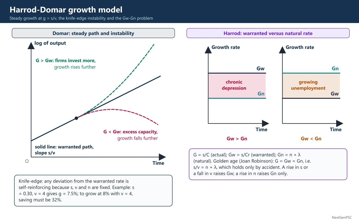
Numerical example: if s = 0.30 and v = 4, then g = 0.30/4 = 7.5% per year; to grow at 8% with v = 4, the saving rate must be 32%.
First problem: instability of the warranted rate (knife-edge). If G exceeds Gw, then C falls short of Cr, firms find capital scarce, invest more, demand rises through the multiplier and G rises further; if G is below Gw, there is excess capacity, investment falls and G falls further, so deviations are cumulative, not self-correcting.
Second problem: Gw versus Gn. If Gw exceeds Gn, the economy cannot sustain Gw because labour runs short, actual growth falls below Gw and there is chronic depression (secular stagnation); if Gw is below Gn, there is growing structural unemployment, though booms are possible.
Golden age (Joan Robinson's phrase): full-employment steady growth requires G = Gw = Gn, i.e. s/v = n + λ, which can hold only by accident since s, v and n are independently given.
Comparative statics: a rise in s raises Gw; a fall in v (better technology or less capital-intensive projects) raises Gw; a rise in n raises Gn but does not change Gw.
Policy implications: poor countries can raise growth by raising saving (domestic effort, foreign aid filling the saving gap) and by lowering the ICOR (efficient use of capital).
3. Criticisms and Limitations
Rigid assumptions: fixed s, v and n with no factor substitution produce instability by construction; Solow (1956) showed that letting v vary through a neoclassical production function removes the knife-edge.
Kaldor's answer (1956): s can adjust because saving propensities of profit earners and wage earners differ, so a shift in income distribution brings Gw towards Gn.
Capital fundamentalism: treats capital as the only engine of growth; ignores technology, human capital, institutions and the efficiency with which capital is used (Easterly's critique of the 'financing gap' model in the 1990s and 2000s).
Harrod's investment function is mechanical: it assumes firms react only to the gap between actual and desired capital, ignoring expectations and the rate of interest.
Closed economy and no government: ignores foreign saving, taxes and public investment.
Relevance for developing countries debated: labour is surplus, so Gn is not binding in the way Harrod assumed; capital is the binding constraint, which made the model look attractive to planners.
4. Diagrams to Draw
Diagram 1 (Domar): put time on the x-axis and the log of output on the y-axis; draw a straight line with slope s/v showing the steady growth path; show actual output above it rising more steeply and output below it falling away, with arrows pointing away from the line to show instability.
Diagram 2 (Harrod knife-edge): draw the saving line S = sY from the origin and an investment line I = Cr ΔY; mark the point where they cross as the warranted path; draw arrows on either side pointing away from the intersection.
Diagram 3 (Gw versus Gn): draw two horizontal lines for Gw and Gn against time; label the region where Gw lies above Gn 'chronic depression' and where Gw lies below Gn 'growing unemployment'.
5. Examples and Applications
India's First Plan (1951–56): used a Harrod-Domar framework with a capital-output ratio of about 3:1 to link a target saving rate to the targeted rise in national income.
ICOR in India: the Planning Commission assumed ICORs of roughly 4 in later plans; a rising ICOR signals that capital is being used less efficiently, a point the Economic Survey and RBI discuss when investment rises without matching growth.
Two-gap model: Chenery and Strout (1966) extended the logic: growth can be held back by a saving gap or a foreign-exchange gap, and foreign aid fills whichever is binding.
East Asia: very high saving and investment rates (often above 35% of GDP) went with fast growth, consistent with the model, though later work stresses productivity as well.
6. Theory and Debates
Harrod versus Domar: Harrod is behavioural (what keeps entrepreneurs satisfied) and focuses on instability; Domar is about the required growth of investment for full use of capacity; both give g = s/v.
Neo-Keynesian response: Kaldor and Joan Robinson made s depend on distribution; neo-classical response: Solow and Swan (1956) made v flexible.
Modern view: the model is a useful accounting framework for planners but a weak theory of long-run growth.
7. Using It in the Exam
10 marks (150 words): state the dual character of investment, derive g = s/v in three lines, give one Indian example.
15 marks (200 words): add Gw, Gn and the knife-edge with one diagram.
20 marks (250 words): assumptions, derivation, the two instability problems, the golden-age condition, criticisms (Solow, Kaldor) and relevance to Indian planning.
Keywords: dual character of investment, warranted rate, natural rate, knife-edge, golden age, ICOR.
Quotable line: Harrod described the warranted path as a 'moving equilibrium' that is highly unstable; Joan Robinson called G = Gw = Gn a 'golden age', a mythical state.
| Rate | Formula | Meaning | What happens if it differs |
|---|---|---|---|
| Actual (G) | G = s/C | Growth actually realised | If G exceeds Gw, cumulative boom; if below, cumulative slump |
| Warranted (Gw) | Gw = s/Cr | Growth that keeps entrepreneurs satisfied | Unstable: the knife-edge |
| Natural (Gn) | Gn = n + λ | Maximum growth allowed by labour and technology | Gw above Gn: stagnation; Gw below Gn: rising unemployment |
Mains points
- Always start from Domar's dual character of investment; it is the logic that produces g = s/v.
- Distinguish clearly between the two problems: instability of Gw (knife-edge) and the gap between Gw and Gn.
- State the assumptions (fixed coefficients, constant s and v); examiners expect you to show that the instability comes from them.
- Give the resolution by Solow (flexible v) and by Kaldor (flexible s) to show breadth.
- Link to India: the First Plan's capital-output ratio and the ICOR debate on investment efficiency.
- Common mistake: calling g = s/v the 'natural rate'; it is the warranted rate.
Did you know?
- Memory trick: 'Save, divide by V' gives the growth rate: g = s/v.
- Harrod himself disliked the 'Harrod-Domar' label because his concern was instability, while Domar's was the investment required for full capacity.
Neo-classical (Solow) and Endogenous Growth: Human Capital and R&D
The Solow-Swan model (1956) allows substitution between capital and labour, so the economy converges to a stable steady state where output per worker grows only at the rate of exogenous technical progress. Endogenous growth theory (Romer 1986, 1990; Lucas 1988) explains that technical progress itself through human capital, knowledge spillovers and purposeful R&D, so policy can change the long-run growth rate.
In simple words
Solow said that adding machines alone cannot make a country rich forever, because each extra machine adds less output; lasting growth needs better technology.
It is like giving a student more and more books: the first few help a lot, later ones little, unless the student learns new ways to study.
Endogenous growth theory says education and research create that technology, so spending on schools and labs pays off.
UPSC asks you to draw the Solow diagram, explain convergence and contrast it with Romer and Lucas.
1. Concepts and Definitions
Solow-Swan model: Robert Solow, 'A Contribution to the Theory of Economic Growth', Quarterly Journal of Economics (1956), and Trevor Swan, 'Economic Growth and Capital Accumulation', Economic Record (1956).
Neo-classical production function: Y = F(K, AL) with constant returns to scale, positive but diminishing marginal products and the Inada conditions; in intensive form y = f(k), where y = Y/AL and k = K/AL.
Steady state: the capital per effective worker k* at which investment just covers break-even investment, so k stops changing.
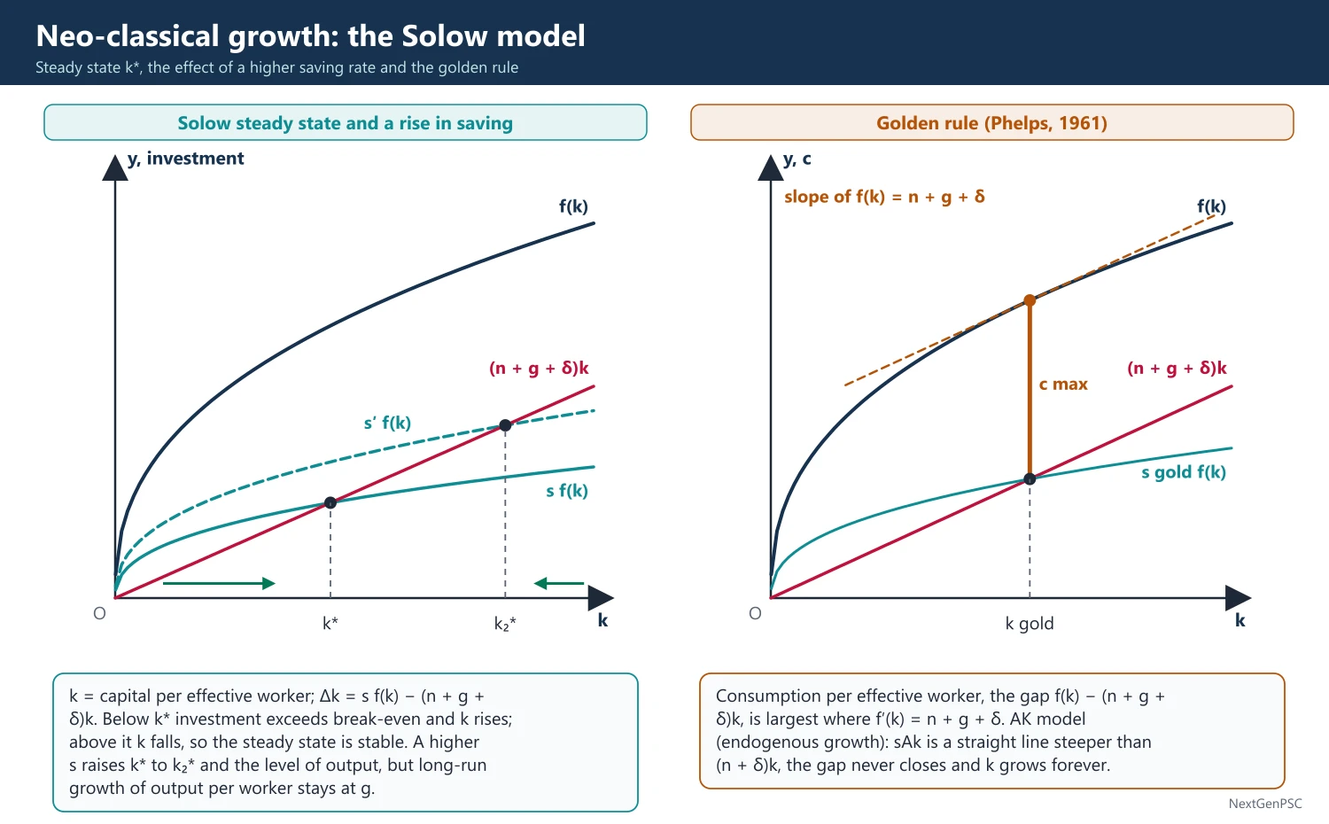
Golden rule (Phelps, 1961): the saving rate that maximises steady-state consumption per worker; it is reached where f′(k) = n + g + δ.
Human capital: the skills, knowledge and health embodied in workers (Schultz 1961; Becker, Human Capital, 1964).
Endogenous growth: theories in which the long-run growth rate is determined inside the model by saving, education, research and policy, not given from outside.
2. The Solow Model Step by Step
Assumptions: closed economy; one good; saving a constant fraction s of output; labour grows at n, labour-augmenting technology at g, capital depreciates at δ; full employment and flexible prices.
Fundamental equation: Δk = s f(k) − (n + g + δ)k; actual investment per effective worker minus break-even investment.
Steady state: s f(k*) = (n + g + δ)k*; at k*, output per effective worker is constant, output per worker grows at g and total output grows at n + g.
Stability: below k*, s f(k) exceeds (n + g + δ)k, so k rises; above k*, k falls; the steady state is globally stable, which removes Harrod's knife-edge because the capital-output ratio adjusts.
Rise in saving rate: raises k* and the level of output per worker, but only temporarily raises growth; the long-run growth rate stays at g (the level effect, not growth effect).
Rise in population growth: lowers k* and output per worker.
Cobb-Douglas case: with y = k^α, k* = [s/(n + g + δ)]^(1/(1 − α)); with α about 1/3, capital's share, the model implies large differences in s and n explain only modest income gaps.
Convergence: absolute (unconditional) convergence means poor countries grow faster than rich ones; conditional convergence means countries converge to their own steady states, given s, n and δ (Barro and Sala-i-Martin, 1990s); evidence supports conditional, not absolute, convergence.
Growth accounting (Solow 1957): ΔY/Y = ΔA/A + α ΔK/K + (1 − α) ΔL/L; the residual ΔA/A, total factor productivity (TFP) growth, explained about seven-eighths of US growth in output per worker in 1909–49, the 'Solow residual'.
3. Limitations of Solow
Technology is exogenous, a 'measure of our ignorance' (Abramovitz); the model explains everything except what drives long-run growth.
It predicts absolute convergence and rates of return on capital in poor countries far higher than observed (Lucas, 'Why doesn't capital flow from rich to poor countries?', 1990).
Mankiw, Romer and Weil (1992) added human capital, y = k^α h^β, and found the augmented model explains about 80% of cross-country income variation, partly rescuing Solow.
4. Endogenous Growth: Human Capital
AK model (Rebelo 1991): Y = AK with no diminishing returns to broad capital (physical plus human); growth g = sA − δ, so a higher saving rate raises growth permanently.
Romer (1986), learning by doing: builds on Arrow (1962); each firm's investment adds to the economy-wide stock of knowledge, so private returns diminish but social returns are constant; spillovers create an externality and the market under-invests.
Lucas (1988), 'On the Mechanics of Economic Development': workers divide time between production and accumulating human capital; ḣ/h = δ(1 − u), where u is time spent working; human capital has an external effect on everyone's productivity, which also explains why skilled people migrate to cities and rich countries.
Policy: public spending on education, health and training raises the growth rate, not just the level; education subsidies correct the externality.
5. Endogenous Growth: Research and Development
Romer (1990), 'Endogenous Technological Change': ideas are non-rival (one person's use does not reduce another's) and partly excludable through patents; firms invest in R&D for monopoly rents; growth depends on the number of researchers and the research productivity: ΔA/A = δ L_A.
Implication: scale effects (more researchers, faster growth), a case for patents to reward innovation and for subsidies to R&D because of knowledge spillovers.
Schumpeterian growth (Aghion and Howitt, 1992): quality-ladder innovations replace old products, Schumpeter's 'creative destruction'; competition and patent policy affect growth.
Jones (1995) critique: the number of US researchers rose sharply while growth did not, so pure scale effects are doubtful; semi-endogenous models make growth depend on population growth.
Nobel recognition: Romer shared the 2018 Nobel for integrating technological innovation into long-run growth; Aghion and Howitt shared the 2025 Nobel (with Joel Mokyr) for innovation-driven growth and creative destruction.
6. Diagrams to Draw
Solow diagram: put k on the x-axis and output and investment per effective worker on the y-axis; draw f(k) concave from the origin, s f(k) below it with the same shape, and the straight line (n + g + δ)k from the origin; mark their intersection k*; show arrows on the k-axis pointing towards k* from both sides.
Rise in s: shift s f(k) up to s′ f(k); mark the new, higher k₂*; beside it draw a time diagram where ln y jumps to a steeper path temporarily, then returns to the original slope g on a higher level.
Golden rule: draw f(k) and (n + g + δ)k; mark kgold where the slope of f(k) is parallel to the break-even line; the vertical gap, consumption, is largest there.
AK model: draw sAk as a straight line steeper than (n + δ)k; the gap never closes, so k grows forever.
7. Examples and Applications
India: studies of growth accounting (for example by Bosworth and Collins, 2008) found that rising TFP contributed substantially to India's growth after 1980, more than in many developing countries.
R&D intensity: India's gross expenditure on R&D has stayed at about 0.6–0.7% of GDP for years (DST data), against about 2.4% in China and above 3% in the US and about 5% in South Korea and Israel, a gap the Economic Survey has repeatedly noted.
Policy responses in India: the Anusandhan National Research Foundation Act, 2023, and a ₹1 lakh crore Research, Development and Innovation fund announced in 2024 aim to raise private R&D.
World: the East Asian debate: Alwyn Young (1995) and Paul Krugman ('The Myth of Asia's Miracle', 1994) argued that East Asian growth was mainly accumulation of inputs, not TFP, so it would slow, a Solow-type prediction.
8. Using It in the Exam
10 marks: state the fundamental equation, steady-state condition and one diagram.
15 marks: add convergence and the effect of a rise in s; contrast with Harrod.
20 marks: Solow, its limits, then Romer, Lucas and AK with policy implications and Indian R&D data.
Keywords: diminishing returns, steady state, golden rule, conditional convergence, Solow residual, non-rival ideas, spillovers, human capital externality.
Quotation: Solow later remarked that 'you can see the computer age everywhere but in the productivity statistics' (1987), the productivity paradox.
| Feature | Solow-Swan (1956) | Endogenous (Romer, Lucas) |
|---|---|---|
| Source of long-run growth | Exogenous technical progress g | Human capital, knowledge spillovers, R&D |
| Returns to capital | Diminishing | Constant to broad capital or to knowledge |
| Effect of higher saving | Level effect only | Can raise growth rate permanently |
| Convergence | Conditional convergence predicted | No necessary convergence; divergence possible |
| Role of policy | Limited in long run | Education, R&D subsidies, patents matter |
Mains points
- The Solow diagram is almost mandatory; label s f(k), (n + g + δ)k and k* clearly.
- Explain why higher saving has a level effect but not a growth effect in Solow; this is the most tested point.
- Use growth accounting and the Solow residual to bridge to endogenous growth.
- For human capital questions cite Schultz, Becker, Lucas (1988) and Mankiw-Romer-Weil (1992).
- For R&D questions explain non-rivalry and spillovers (Romer 1990) and give India's R&D-to-GDP ratio with source.
- Common mistake: saying Solow predicts absolute convergence for all countries; the robust prediction is conditional convergence.
Did you know?
- Robert Solow won the 1987 Nobel; Paul Romer won it in 2018 for 'endogenising' the very technology Solow left outside the model.
- Memory trick: Solow = 'Slow down' (diminishing returns); Romer = 'Recipes' (ideas that never run out).
Lewis Model of Development with Surplus Labour (and Ranis-Fei)
W. Arthur Lewis (1954) modelled a dual economy: a traditional subsistence sector with surplus labour whose marginal product is near zero, and a modern capitalist sector that hires them at a constant wage slightly above subsistence. Reinvested profits expand the modern sector until surplus labour is absorbed at the Lewis turning point. Ranis and Fei (1961) added the agricultural surplus and three phases.
In simple words
The Lewis model says poor countries have too many people on farms; some can leave without farm output falling, because their extra work adds almost nothing (disguised unemployment).
It is like five people sharing a job that three can do: two can take factory jobs and the field still gets ploughed.
Factories hire them at a steady wage, earn profits, reinvest, and the economy industrialises.
UPSC asks you to draw the Lewis diagram, explain the turning point and test it against India's slow shift of workers out of farming.
1. Concepts and Definitions
Source: W. Arthur Lewis, 'Economic Development with Unlimited Supplies of Labour', The Manchester School (1954); Lewis shared the 1979 Nobel with Theodore Schultz.
Dual economy: a subsistence (traditional, largely agricultural, family-based) sector and a capitalist (modern, wage-employing, profit-reinvesting) sector, which may include plantations and mines, not only factories.
Unlimited supply of labour: at the going wage, labour supply to the modern sector is perfectly elastic because the subsistence sector holds surplus labour.
Surplus labour or disguised unemployment: workers whose marginal product (MPL) is zero or negligible, so their withdrawal does not reduce output; the idea also appears in Nurkse (1953) as a hidden saving potential.
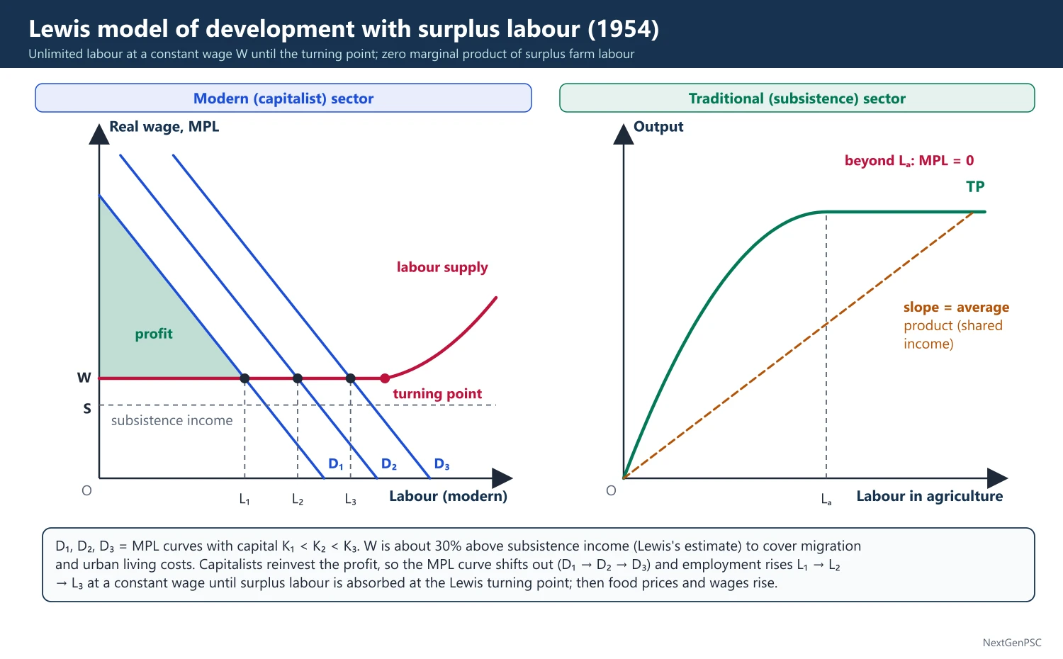
Institutional or subsistence wage: in the traditional sector income is shared, so the wage equals the average product, not the marginal product; the modern sector must pay about 30% more (Lewis's estimate) to cover migration costs and higher urban living costs.
2. The Model Step by Step
Assumptions: surplus labour in agriculture; constant real wage in the modern sector until surplus is exhausted; capitalists save and reinvest all profits; workers save nothing; labour moves freely; no technical progress that saves labour.
Stage 1: the modern sector hires up to where MPL equals the constant wage W; the area under the MPL curve above W is capitalists' surplus (profit).
Stage 2: profits are reinvested, raising the capital stock from K1 to K2, which shifts the MPL curve outward; more workers are hired at the same wage, and the profit share of national income rises.
Key result: the central problem of development, in Lewis's words, is to understand how a community that saved 4 or 5% of national income becomes one that saves 12 or 15%; the rise in the profit share explains the rise in saving.
Lewis turning point: once surplus labour is absorbed, the MPL in agriculture becomes positive, agricultural output falls when labour leaves, food prices rise, and the modern sector faces an upward-sloping labour supply; wages start rising and the dual economy becomes one integrated, neo-classical economy.
Terms-of-trade problem: if agricultural output stagnates, food prices rise relative to manufactures and push up the industrial wage early, choking profits; Lewis recognised that agricultural productivity must rise alongside industry.
3. Ranis-Fei Extension (1961)
Source: Gustav Ranis and John C. H. Fei, 'A Theory of Economic Development', American Economic Review (1961), and their book Development of the Labor Surplus Economy (1964).
Phase I: MPL in agriculture is zero; labour moves to industry without reducing farm output; the total agricultural surplus (output not consumed by those who remain) is available to feed industrial workers at the institutional wage.
Phase II: MPL is positive but below the institutional wage (disguised unemployment remains); as labour leaves, farm output falls, the average agricultural surplus per industrial worker drops, food prices rise and the industrial wage starts rising; the first point is the 'shortage point'.
Phase III: MPL exceeds the institutional wage; agriculture is commercialised, wages are set by the market in both sectors; the start of this phase is the 'commercialisation point'.
Balanced growth condition: to avoid the shortage point arriving early, agricultural productivity must rise (technical progress shifts the total product curve up), so that the shortage and commercialisation points merge; industrial and agricultural growth must be balanced.
Critical minimum effort: industrial labour absorption must exceed population growth for the economy to move out of the labour-surplus stage.
4. Criticisms and Limitations
Labour-saving investment: if profits are reinvested in capital-intensive technology, the MPL curve shifts up but becomes steeper and employment barely grows (Todaro and Smith); jobless growth.
Urban unemployment: the model assumes full employment in cities; Harris and Todaro (1970) showed that migration responds to expected urban income, creating open urban unemployment and informal sectors.
Constant urban wage: union pressure, minimum wages and civil-service pay raise urban wages even with surplus labour.
Existence of zero MPL debated: T. W. Schultz, in Transforming Traditional Agriculture (1964), used the 1918–19 influenza epidemic in India to argue that farm output fell when labour fell, so MPL was not zero; A. K. Sen (1966) argued that surplus labour can exist in labour hours even if not in workers.
Capital flight: profits may be sent abroad or used for consumption, not reinvested locally.
Neglect of agriculture: Lewis himself treated agriculture as a passive reservoir; Ranis-Fei and Jorgenson (1961) gave agriculture an active role.
5. Diagrams to Draw
Lewis diagram: upper panel: x-axis labour in the modern sector, y-axis real wage and MPL; draw the labour supply curve horizontal at W (above subsistence wage S) and then turning upward at the turning point; draw MPL curves D1(K1), D2(K2), D3(K3) shifting outward; employment rises from L1 to L2 to L3; shade the area above W under each MPL curve as profit.
Lower panel (agriculture): x-axis labour in agriculture, y-axis output; draw the total product curve rising and then flat beyond point L_A, showing zero MPL; mark the average-product line whose slope is the subsistence wage.
Ranis-Fei diagram: three panels aligned vertically: industrial labour market, agricultural total product, and agricultural MPL with the institutional wage line; mark the shortage point and commercialisation point and show how technical progress in agriculture shifts the total product curve up so the points coincide.
6. Examples and Applications
China: the Lewis turning point debate: Cai Fang and others argued China reached the turning point around 2004–2010 when rural migrant wages began rising fast; others disputed it.
South Korea and Taiwan: Ranis and Fei used Taiwan; labour-intensive manufacturing absorbed surplus labour by the 1970s, after which real wages rose rapidly.
India: agriculture's share of employment fell slowly while its share of GVA fell fast; PLFS shows agriculture employing about 46% of workers in 2023–24 (PLFS annual report) while contributing about 16–18% of GVA, a sign of surplus labour; manufacturing absorbed little and construction and services took most of the movers.
India's reverse migration: the share of workers in agriculture rose after 2019–20 (about 42.5% in 2018–19 to about 46% in 2023–24, PLFS), the opposite of the Lewis path, partly due to the COVID-19 shock.
7. Related Models
Jorgenson (1961) neo-classical dual model: Dale Jorgenson denied zero MPL and a fixed wage; the agricultural surplus arises only from technical progress in agriculture, the modern sector's growth depends on that surplus, and wages rise steadily.
Harris-Todaro condition (1970): migration continues until the rural wage equals the expected urban wage, Wr = (Le/Lu) × Wu, where Le/Lu is the probability of getting a modern-sector job; creating more urban jobs can raise urban unemployment by attracting more migrants (the Todaro paradox).
Policy lesson for India: labour-intensive manufacturing (textiles, apparel, footwear, food processing, electronics assembly) is the channel the Lewis model calls for, and the Economic Survey has repeatedly argued for it.
8. Using It in the Exam
10 marks: define dual economy and surplus labour, describe the horizontal labour supply and reinvestment, one line on the turning point.
15 marks: add the diagram and two criticisms (Harris-Todaro, labour-saving technology).
20 marks: Lewis, Ranis-Fei phases, criticisms (Schultz, Sen), and evidence from China and India with PLFS data.
Keywords: unlimited supplies of labour, institutional wage, capitalist surplus, Lewis turning point, shortage point, commercialisation point.
Attributed idea: Lewis held that the key to development is the rise of the saving rate through the growing share of profits in national income.
| Feature | Lewis (1954) | Ranis-Fei (1961) |
|---|---|---|
| Role of agriculture | Passive reservoir of labour | Active: supplies food surplus and must modernise |
| Phases | Two: surplus labour, then turning point | Three: zero MPL, MPL below wage, MPL above wage |
| Key points | Lewis turning point | Shortage point and commercialisation point |
| Condition for success | Reinvestment of profits | Balanced growth of agricultural productivity and industrial employment |
Mains points
- Draw the Lewis two-panel diagram; it is the core of any answer.
- Explain why the wage stays constant (average-product sharing, institutional wage) and why profits rise as a share of income.
- Add Ranis-Fei phases to show that agriculture must modernise; examiners reward this extension.
- Use Harris-Todaro and labour-saving technology as the main criticisms; mention Schultz's influenza evidence and Sen's reply.
- Test against India with PLFS data on agricultural employment and the weak absorption by manufacturing.
- Common mistake: assuming surplus labour means unemployed people; in Lewis they are employed but with near-zero marginal product.
Did you know?
- Arthur Lewis, born in St Lucia in the Caribbean, was the first Black person to win a Nobel Prize in a field other than peace (economics, 1979).
Balanced and Unbalanced Growth: Rosenstein-Rodan, Nurkse and Hirschman
Balanced growth theorists (Rosenstein-Rodan's Big Push, 1943; Nurkse, 1953) argued that a poor economy must invest simultaneously in many complementary industries, because each alone faces too small a market. Albert Hirschman (1958) replied with unbalanced growth: invest deliberately in key sectors with strong linkages, and the shortages and pressures created will induce investment elsewhere.
In simple words
Balanced growth says: open many factories together, because workers in each will buy the others' goods; one shoe factory alone in a poor village would find too few buyers. This is the Big Push.
Unbalanced growth says: build a steel plant or a dam first; the shortages it creates will push others to invest nearby.
Both matter because poor countries have small markets and little capital.
UPSC asks you to compare the two and judge which fits India's planning.
1. Concepts and Definitions
Big Push: Paul Rosenstein-Rodan, 'Problems of Industrialisation of Eastern and South-Eastern Europe', Economic Journal (1943): a minimum, large, coordinated investment programme is needed to overcome indivisibilities and launch development; 'proceeding bit by bit will not add up in its effects to the sum total of the single bits' (paraphrase of his argument).
Indivisibilities (Rosenstein-Rodan): (1) in the production function, especially social overhead capital such as power, transport and irrigation, which comes in large lumps; (2) in demand, because industries are complementary buyers of each other's output; (3) in the supply of savings, since a high minimum investment needs a jump in saving.
Pecuniary external economies (Scitovsky, 1954): the profit of one industry depends on the investment of others through prices and markets; these justify coordinated investment that a market of isolated decisions would not undertake.
Vicious circle of poverty (Nurkse): Ragnar Nurkse, Problems of Capital Formation in Underdeveloped Countries (1953): 'a country is poor because it is poor'; on the supply side low income → low saving → low capital → low productivity → low income; on the demand side low income → small market → low inducement to invest → low productivity → low income.
Balanced growth (Nurkse): a wave of investments in a number of different industries, so that people working in each become customers of the others; based on Say's Law applied to a whole range of goods and on the size of the market (Adam Smith, Allyn Young 1928).
Unbalanced growth (Hirschman): Albert O. Hirschman, The Strategy of Economic Development (1958): development is a chain of disequilibria; the scarce resource is decision-making ability, so deliberately unbalancing the economy creates pressures that induce decisions.
2. The Balanced Growth Model Step by Step
Rosenstein-Rodan's shoe-factory example: 20,000 unemployed workers in a shoe factory would not buy all the shoes, so the factory fails; if a million workers are employed across many industries producing the goods they consume, they form each other's market.
Role of the state: since private investors coordinate poorly, the state should plan and finance a big push, especially in social overhead capital.
Nurkse's emphasis: balanced growth on the demand side across consumer-goods industries; he also stressed using disguised unemployment as a source of saving (workers moved to capital projects while those who remain feed them).
Lewis and Scitovsky: also supported balanced growth between agriculture and industry, so the terms of trade do not move against industry.
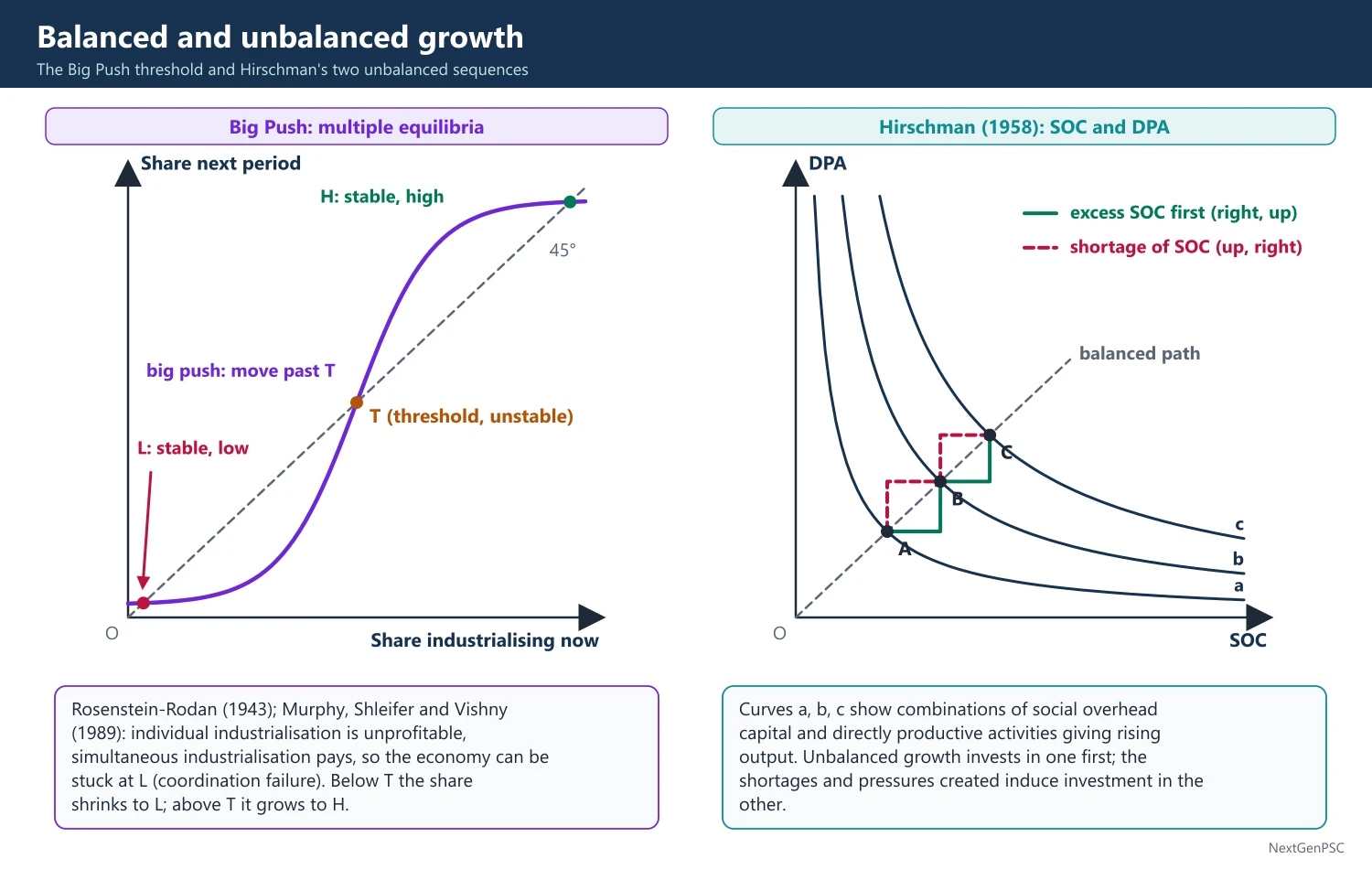
Modern formalisation: Murphy, Shleifer and Vishny, 'Industrialization and the Big Push', Journal of Political Economy (1989), showed multiple equilibria: if firms using increasing-returns technology pay higher wages, simultaneous industrialisation can be profitable while individual industrialisation is not; the economy can be stuck in a low-level equilibrium (a coordination failure).
3. The Unbalanced Growth Model Step by Step
Social overhead capital (SOC) and directly productive activities (DPA): development can proceed through excess SOC (build power and roads first, which make DPA cheap and attract private investment) or through shortage of SOC (build DPA first; the bottlenecks create political pressure for SOC).
Hirschman's preference: development via shortage is more compelling because it creates strong pressures, though he allowed that excess SOC is safer.
Linkages: a backward linkage is the demand an industry creates for inputs (steel → iron ore, coal); a forward linkage is the supply it provides as inputs to others (steel → machinery, construction).
Investment priority: invest first in industries with the highest total linkages; Hirschman used input-output data (Chenery and Watanabe) to show that iron and steel, paper, petroleum products, leather and textiles have high linkages, while agriculture has weak backward linkages.
Induced decisions: each disequilibrium (shortage, profit opportunity, political pressure) induces the next investment, so the economy moves in a 'see-saw' advance.
Paul Streeten (1959) and Singer: also favoured unbalanced growth as a realistic strategy for capital-scarce countries.
4. Criticisms
Of balanced growth: (1) poor countries lack the capital, skills and administrative capacity for a simultaneous big push; Hirschman and Singer argued it is a cure for a stage of underdevelopment that the economy has already passed; (2) it ignores foreign trade, which can provide the market (export-led growth of East Asia); (3) it can produce inefficient, high-cost industries; (4) Kurihara and others noted it is more relevant for advanced economies in depression than for poor countries.
Of unbalanced growth: (1) bottlenecks may simply cause inflation and balance-of-payments crises instead of inducing investment; (2) it neglects agriculture, which has weak linkages but feeds the workforce; (3) political pressure may not produce efficient responses; (4) the distinction between SOC and DPA is not always sharp.
Synthesis: the two are seen as complementary in practice: balance is the goal, imbalance is a path; Streeten called unbalanced growth 'balanced growth over time'.
5. Diagrams to Draw
Big Push multiple equilibria: plot expected profit (or the share of firms that industrialise next period) on the y-axis against the share that industrialise now on the x-axis; draw an S-shaped curve crossing the 45° line at three points: a stable low equilibrium near zero, an unstable middle point (threshold), and a stable high equilibrium; a big push moves the economy past the threshold.
Hirschman's SOC-DPA diagram: put SOC on the x-axis and DPA on the y-axis; draw curves a, b, c showing combinations giving rising output levels and a 45° expansion path of balanced growth; show a staircase path that first moves right (excess SOC) and then up (DPA catches up), and an alternative staircase that first moves up (shortage of SOC) then right.
Vicious circle: draw two circles of arrows: supply side (low income → low saving → low investment → low capital → low productivity → low income) and demand side (low income → low demand → low inducement to invest → low capital → low productivity → low income).
6. Examples and Applications
India's Second Plan (1956–61): the Mahalanobis strategy concentrated investment in heavy industry (steel plants at Bhilai, Rourkela, Durgapur), close to Hirschman's emphasis on high-linkage sectors while relying on the state as in the Big Push; it ran into a foreign-exchange crisis in 1957–58, a bottleneck of the kind critics warned of.
Infrastructure-led push today: India's public capital expenditure push since 2020–21 (Union capex of about ₹11.2 lakh crore budgeted for 2025–26), the PM Gati Shakti National Master Plan (2021) and dedicated freight corridors are an SOC-first strategy in Hirschman's terms.
Production Linked Incentive schemes (2020 onward): targeting electronics, mobile phones and other high-linkage sectors resemble a selective, unbalanced strategy.
World: South Korea's heavy and chemical industry drive (1973–79) and the Soviet industrialisation under the Five-Year Plans are cited as big-push cases; Taiwan's growth with labour-intensive exports is cited against the need for a domestic big push.
7. Related Theories
Perroux's growth poles (1955): François Perroux argued that growth appears first at poles of propulsive industries and spreads unevenly, an idea close to Hirschman's linkages.
Trickle-down versus backwash: Hirschman expected growth at the poles to produce trickling-down effects as well as polarisation effects on backward regions, while Myrdal (1957) stressed backwash effects that widen regional gaps.
Leibenstein's critical minimum effort (1957): Harvey Leibenstein argued that an effort large enough for income-raising forces to outweigh income-depressing forces such as population growth is needed, close in spirit to the Big Push.
Nelson's low-level equilibrium trap (1956): Richard Nelson showed that when population growth outpaces income growth at low incomes, small rises in income per head are wiped out, so a large push is needed to escape.
Rostow's take-off: W. W. Rostow, The Stages of Economic Growth (1960), required the investment rate to rise from about 5% to over 10% of national income with leading sectors, combining big-push and leading-sector ideas.
Role of trade: later trade-oriented critics argued that in an open economy world markets relax the demand constraint for traded goods, so coordinated investment matters most for non-traded infrastructure.
8. Using It in the Exam
10 marks: define both, one line each on Rosenstein-Rodan, Nurkse and Hirschman, one Indian example.
15 marks: add indivisibilities, linkages and two criticisms each.
20 marks: structured comparison, diagrams (S-curve, SOC-DPA staircase), India's Second Plan and today's capex push, conclude that they are complementary.
Keywords: indivisibilities, pecuniary external economies, vicious circle of poverty, size of the market, linkages, SOC and DPA, coordination failure.
Attributed line: Nurkse's 'a country is poor because it is poor' sums up the vicious circle; Hirschman's view was that development depends less on finding optimal combinations of resources than on calling forth resources that are hidden, scattered or badly utilised (paraphrase).
| Feature | Balanced (Rosenstein-Rodan, Nurkse) | Unbalanced (Hirschman, Streeten, Singer) |
|---|---|---|
| Main constraint | Small size of the market, indivisibilities | Scarcity of decision-making ability |
| Strategy | Simultaneous investment across many industries | Investment in key high-linkage sectors |
| Role of disequilibrium | To be avoided | Deliberately created to induce investment |
| Resource need | Very large, all at once | Smaller, sequential |
| Main criticism | Poor countries cannot afford it; ignores trade | Bottlenecks may cause inflation and BoP crises |
Mains points
- Name the three indivisibilities of Rosenstein-Rodan; this is a frequently tested detail.
- Explain Nurkse's vicious circle on both supply and demand sides with a quick flow diagram.
- Define backward and forward linkages with Indian examples (steel, petrochemicals, electronics).
- Present SOC versus DPA routes in Hirschman with the staircase diagram.
- Conclude that the strategies are complementary, citing Streeten, and link to India's Second Plan and present capex-led growth.
- Common mistake: treating Nurkse's balanced growth as balanced between agriculture and industry only; it is primarily about complementary consumer-goods industries and the size of the market.
Did you know?
- Rosenstein-Rodan illustrated the Big Push with an airplane: it must reach a critical ground speed before it can become airborne.
- Memory trick: Nurkse = 'Need a Net of industries'; Hirschman = 'Hit the Hub (linkages) first'.
UPSC Previous Year Questions: Theories of Growth
From 2014 to 2026 UPSC asked 35 question parts (540 marks) from Theories of Growth, making it one of the heaviest chapters of Paper I. Solow and endogenous growth (human capital, R&D, golden rule, Solow residual: 15 parts) and the Harrod-Domar model (warranted and natural rates, knife-edge: 8 parts) lead, followed by balanced versus unbalanced growth and the Lewis model. Every question below has a model answer written to the UPSC word limit.
In simple words
Read the question and spend five minutes writing your own outline: the model, its equation, the diagram and a conclusion.
Then read the model answer and tick what you missed: the economist and year, the steady-state or warranted-rate condition, the diagram or the derivation step.
Practise derivations (Domar's exponential path, Solow's steady state, golden rule, two-sector R&D model) on paper until you can write them without notes.
1. Harrod-Domar Model
Example 1 (UPSC 2025, 10 marks): Write down the implications of knife-edge problem in Harrod's model of growth.
Paper and question: Paper I, Q5(d)
Approach: State the knife-edge (instability of the warranted path) briefly and then list its implications for the economy and for policy.
In Harrod's model (1939) steady growth requires the actual rate G to equal the warranted rate Gw = s/Cr. Any deviation is self-reinforcing: if G exceeds Gw, the actual capital-output ratio is below the required Cr, firms invest more and G rises further; if G is below Gw, excess capacity cuts investment and G falls further. This is the knife-edge.
Implications: (i) steady growth is a matter of chance, since the economy is unlikely to stay on the warranted path; (ii) capitalist economies are inherently unstable and prone to cumulative booms and slumps; (iii) a rise in thrift raises Gw and, if G does not follow, leads to depression, a growth version of Keynes's paradox of thrift.
(iv) Because Gw also rarely equals the natural rate Gn, full-employment growth is unlikely without policy, so government must use fiscal and monetary policy to keep G close to Gw.
The knife-edge stimulated later models: Solow (1956) removed it with a variable capital-output ratio, and Kaldor with a variable saving ratio.
Example 2 (UPSC 2025, 15 marks): Define the concept of natural growth in Harrod's model. What are the implications of deviation of actual growth from natural growth?
Paper and question: Paper I, Q7(c)
Approach: Define Gn with its determinants, then explain the two cases of deviation (actual or warranted growth above and below Gn) and their consequences, with the policy implication.
In Harrod's model the natural rate of growth Gn is the maximum long-run rate permitted by the growth of the labour force and labour-augmenting technical progress: Gn = n + λ, where n is population (labour force) growth and λ the rate of technical progress. It is the rate that maintains full employment.
Gn is a ceiling: actual growth can exceed Gn only temporarily, by absorbing unemployed labour, after which it is pulled back to Gn.
Case 1, G (and Gw) above Gn: output cannot grow faster than labour and technology allow for long. When G is pulled down to Gn it falls below Gw, firms find excess capacity, cut investment, and the economy tends to secular stagnation. This fits mature high-saving economies; the remedy is to lower s or raise public investment.
Case 2, G (and Gw) below Gn: capital grows too slowly to employ the growing labour force, so there is chronic structural unemployment of labour together with a tendency for G to exceed Gw, i.e. inflationary pressure and booms. This fits developing countries with high population growth and low saving; the remedy is to raise s through saving mobilisation.
Thus full-employment steady growth requires G = Gw = Gn, which Joan Robinson called a 'golden age', a mythical state, since s, Cr and n are determined independently. Solow and Kaldor later showed how Gw could adjust towards Gn.
Example 3 (UPSC 2024, 15 marks): Distinguish between warranted rate of growth and natural rate of growth. Explain how knife-edge instability problem occurs in Harrod's model of economic growth.
Paper and question: Paper I, Q8(c)
Approach: Define and distinguish Gw and Gn (meaning, determinants, nature), then explain the knife-edge between actual and warranted growth with its mechanism.
Warranted rate (Gw): in Harrod's model (1939) it is the growth rate at which entrepreneurs are satisfied that they have invested the right amount, so that saving equals desired investment and the actual capital-output ratio equals the required ratio Cr: Gw = s/Cr. It depends on behaviour (saving propensity and technology).
Natural rate (Gn): the maximum rate permitted by labour-force growth and technical progress, Gn = n + λ; it maintains full employment and depends on demography and technology. Gw is an equilibrium of the goods market and capacity use, Gn a full-employment ceiling; there is no mechanism making them equal.
Knife-edge instability: the actual rate is given by the identity G·C = s. Suppose G exceeds Gw. Since s is the same, C must be below Cr: capital is short relative to output, so firms raise investment. Through the multiplier this raises demand and G further, pushing it even further above Gw. If G is below Gw, C exceeds Cr, firms have idle capacity, cut investment, demand falls and G falls further.
Diagram: growth rate on the vertical axis and time on the horizontal; a horizontal line at Gw; paths starting slightly above Gw diverge upwards and paths starting slightly below diverge downwards, like a ball on a knife's edge.
The instability arises because investment follows the accelerator (it responds to the gap between actual and required capital) while the capital-output ratio and saving ratio are fixed. Solow (1956) removed it with factor substitution.
Example 4 (UPSC 2022, 10 marks): Show that in Domar's growth model, in equilibrium, path of investment is exponential.
Paper and question: Paper I, Q5(d)
Approach: Set out Domar's supply side (σI) and demand side (ΔI/α), equate them and solve the differential equation to get I(t) = I₀e^(ασt).
Evsey Domar (1946) stressed the dual character of investment: it adds to productive capacity and it generates income through the multiplier. Equilibrium growth requires the increase in demand to equal the increase in capacity.
Step 1 (supply side): capacity P rises with investment: dP/dt = σI, where σ is the potential social average productivity of investment (output-capital ratio).
Step 2 (demand side): by the multiplier, dY/dt = (1/α)(dI/dt), where α is the marginal propensity to save.
Step 3 (equilibrium): set dY/dt = dP/dt: (1/α)(dI/dt) = σI, so (dI/dt)/I = ασ.
Step 4 (solution): integrating, ln I = ασt + constant, so I(t) = I₀e^(ασt), where I₀ is initial investment.
In words: to keep capacity fully used, investment (and with it income) must grow exponentially at the constant required rate ασ. For example, with α = 0.12 and σ = 0.25, investment must grow at 3% a year. If investment grows more slowly, idle capacity appears and investment is discouraged further; Domar's equilibrium, like Harrod's, is therefore unstable.
Since α = s and σ = 1/v, the required rate equals Harrod's warranted rate s/v.
Example 5 (UPSC 2022, 15 marks): What do you mean by the warranted rate of growth? Explain the knife edge instability problem in Harrod's growth model.
Paper and question: Paper I, Q6(a)
Approach: Define Gw with its derivation (S = sY, I = CrΔY), then explain the knife-edge mechanism in both directions with a diagram and the reason behind it.
The warranted rate of growth (Harrod, 1939) is the rate of growth of income which, if achieved, would leave entrepreneurs satisfied that they have produced and invested the right amount, so they continue on the same path.
Derivation: saving S = sY; desired investment depends on the increase in output, I = Cr·ΔY (accelerator), where Cr is the required capital-output ratio. Equilibrium S = I gives sY = Cr·ΔY, so Gw = ΔY/Y = s/Cr. With s = 0.2 and Cr = 4, Gw = 5%.
Knife-edge: the actual rate satisfies G·C = s ex post. If G exceeds Gw, the actual C is below Cr: firms find they have too little capital, raise investment, and the multiplier raises demand, so G moves further above Gw. If G is below Gw, C exceeds Cr, there is surplus capacity, investment falls and G falls further. The warranted path is an unstable equilibrium: departures are cumulative, not self-correcting.
Diagram: time on the horizontal axis and growth rate on the vertical; a horizontal line at Gw; arrows from points above it move upwards and from points below it move downwards.
The root cause is the combination of fixed s and Cr with an accelerator investment function. Solow (1956) and Swan (1956) made the capital-output ratio flexible and Kaldor made s depend on distribution, which restores stability.
Example 6 (UPSC 2021, 20 marks): Explain how Harrod's warranted rate of growth is similar to Domar's required rate of growth. How has Solow improved upon Harrod-Domar's growth model?
Paper and question: Paper I, Q6(c)
Approach: Derive Gw = s/Cr and Domar's ασ, show they are the same expression under stated equivalences and note differences; then explain Solow's improvements (factor substitution, stable steady state, role of technology) with the diagram.
Similarity: Harrod's warranted rate comes from equating saving sY with accelerator investment Cr·ΔY, giving Gw = s/Cr. Domar's required rate comes from equating the growth of demand (1/α)ΔI with the growth of capacity σI, giving ΔI/I = ασ. Since Domar's α is the saving ratio s and his σ is the output-capital ratio 1/v, ασ = s/v: both are the rate at which income must grow so that saving is absorbed by investment and capacity is fully used. Both assume a fixed saving ratio, a fixed capital-output ratio, no technical change and a closed economy, and both equilibria are unstable.
Difference: Harrod works with income and entrepreneurs' expectations (actual, warranted and natural rates), whereas Domar works with investment and its dual character and does not use the accelerator.
Solow's improvements (1956): (i) a neoclassical production function Y = F(K, L) with constant returns and diminishing returns to each factor allows factor substitution, so the capital-output ratio becomes variable; (ii) the fundamental equation k̇ = sf(k) − (n + δ)k gives a unique, stable steady state where sf(k*) = (n + δ)k*, removing the knife-edge, because Gw adjusts to Gn through changes in k; (iii) long-run growth of per capita income depends on technical progress, not on the saving rate, which only affects the level; (iv) the model predicts conditional convergence and allows growth accounting (the Solow residual).
Diagram: k on the horizontal axis; the curve sf(k) concave and the ray (n + δ)k; they intersect at k*; to the left sf(k) lies above the ray and k rises, to the right it lies below and k falls, so k* is stable.
Solow's own limitation is that technical progress is exogenous, which endogenous growth theory (Romer, Lucas) later addressed.
Example 7 (UPSC 2018, 10 marks): In Harrod's model of growth, if the expected growth rate exceeds the warranted growth rate, what will be the relation between the actual growth rate and the expected growth rate?
Paper and question: Paper I, Q5(c)
Approach: State the result (actual growth exceeds expected growth) and explain the mechanism through the multiplier and the capital-output ratio, then its consequence.
In Harrod's model entrepreneurs invest according to the growth they expect (Ge). The warranted rate Gw = s/Cr is the rate at which expectations are just fulfilled.
If Ge exceeds Gw, the actual growth rate exceeds the expected rate. Firms invest enough to equip the expected growth (I = Cr·Ge·Y), which is more than the saving the economy would generate at the warranted rate. Through the multiplier, this extra investment raises demand and output by more than firms expected; ex post G·C = s, so with G higher the actual capital-output ratio falls below Cr.
Firms therefore find their expectations exceeded and capital short, so they revise Ge upwards and invest still more. The gap widens, giving a cumulative boom; symmetrically, if Ge is below Gw, actual growth falls short of expectations and a cumulative slump follows.
This is the expectational form of Harrod's knife-edge: deviations from the warranted path are self-reinforcing, not self-correcting.
Example 8 (UPSC 2015, 10 marks): Do you think that the root of Harrod's instability problem lies in the assumption of wage-price rigidity? Give arguments in favour of your answer.
Paper and question: Paper I, Q5(a)
Approach: Give a qualified answer: neoclassicals trace the instability to rigid factor prices and fixed coefficients, but the knife-edge itself comes from the investment (accelerator) behaviour; argue both sides and conclude.
Partly. Harrod's instability has two parts: the knife-edge between actual and warranted growth, and the gap between warranted and natural growth.
In favour: Solow (1956) argued that the problem comes from fixed coefficients, i.e. a fixed capital-output ratio. If wages and the rate of interest were flexible, a shortage of labour would raise wages relative to interest, firms would adopt more capital-intensive techniques, and the capital-output ratio would adjust until Gw = s/v equals Gn. Kaldor similarly showed that flexible prices change income distribution and hence the saving ratio. So rigid factor prices underlie the Gw-Gn problem.
Against: the knife-edge between G and Gw arises from the accelerator-based investment function and entrepreneurs' expectations: when growth exceeds the warranted rate, firms invest more, which raises growth further. This is a problem of effective demand that wage-price flexibility does not remove; falling wages may even reduce demand, as Keynes argued.
Hence wage-price rigidity explains the long-run divergence of warranted and natural rates, but the short-run knife-edge lies in investment behaviour.
2. Neo-classical (Solow) and Endogenous Growth: Human Capital and R&D
Example 9 (UPSC 2026, 10 marks): Analyse the role of Research and Development (R&D) in fostering economic growth and strengthening competitiveness in a knowledge-based economy.
Paper and question: Paper I, Q5(d)
Approach: Explain how R&D drives growth (non-rival ideas, increasing returns, spillovers, as in Romer) and how it builds competitiveness, with Indian data and a short conclusion.
In a knowledge-based economy, growth depends on the production of new ideas. Paul Romer (1990) made technology endogenous: firms invest in R&D to earn monopoly profits from new designs, and the stock of ideas grows as Ȧ = δL_A·A, so long-run growth depends on the resources devoted to research.
Growth channels: ideas are non-rival, so one design can be used across the economy at no extra cost, giving increasing returns; knowledge spills over to other firms and future researchers; and R&D raises total factor productivity, which explains most long-run growth of income per head.
Competitiveness: R&D creates new products and lowers costs, giving a dynamic comparative advantage (as in Korea's electronics and Taiwan's semiconductors) and the absorptive capacity to adopt foreign technology.
India spends only about 0.64% of GDP on R&D (Department of Science and Technology data for 2020–21), far below China and Korea, and business funds a small share. Schemes such as the Anusandhan National Research Foundation Act, 2023 aim to raise this. Strong patents, universities and industry links are needed.
Example 10 (UPSC 2026, 20 marks): Analyse the role of human capital as a driver of economic development in developing countries. How can education and healthcare investment overcome the "Low productivity trap" in developing nations?
Paper and question: Paper I, Q7(a)
Approach: Define human capital (Schultz, Becker) and its growth channels (Lucas, Mankiw-Romer-Weil, Nelson-Phelps), explain the low-productivity trap as a vicious circle, then show how education and health investments break it, with Indian policy examples.
Human capital is the stock of skills, knowledge and health embodied in people that raises their productivity. Theodore Schultz ('Investment in Human Capital', 1961) and Gary Becker (Human Capital, 1964) treated education and health as investments with measurable returns.
Role in development: (i) it raises labour productivity directly; (ii) in Lucas (1988), human capital accumulates without diminishing returns and has external effects, sustaining long-run growth; (iii) in Mankiw, Romer and Weil (1992), adding human capital to the Solow model explains most cross-country income differences; (iv) Nelson and Phelps (1966) showed that educated workers adopt new technologies faster.
Low-productivity trap: low education and poor nutrition keep productivity and wages low; low incomes prevent families from investing in schooling and health; and the next generation is again unproductive. Nutrition-based efficiency wage theory (Leibenstein; Dasgupta and Ray) shows that poorly fed workers cannot work productively, so the poor cannot earn enough to become better fed: a self-reinforcing equilibrium.
Breaking the trap: public investment is needed because credit constraints and externalities prevent private investment. Education: universal schooling with a focus on foundational literacy and numeracy (India's NEP 2020 and NIPUN Bharat), vocational skills and higher education quality. Health: nutrition (mid-day meals, Poshan Abhiyaan from 2018), immunisation, sanitation and insurance (Ayushman Bharat-PMJAY from 2018), which raise working capacity and children's learning. Evidence such as deworming in Kenya (Miguel and Kremer, 2004) shows large gains from cheap health inputs.
These investments raise productivity, earnings and the capacity to invest, turning a vicious circle into a virtuous one, as in East Asia, Kerala's social development and China. Their returns are long-term, so they need sustained public funding and attention to quality, not just enrolment.
Example 11 (UPSC 2025, 20 marks): Analyse critically the role of human capital and Research and Development (R&D) expenditure on economic growth in the framework of endogenous growth model.
Paper and question: Paper I, Q7(a)
Approach: Set out why endogenous growth theory was needed, then the human-capital channel (Lucas) and the R&D channel (Romer) with their equations, and critically assess (scale effects, Jones's critique, evidence, policy).
In the Solow model long-run growth of income per head equals the exogenous rate of technical progress, and diminishing returns to capital stop growth from saving. Endogenous growth theory explains growth from within the model by finding inputs that do not suffer diminishing returns.
Human capital (Lucas, 1988): output is Y = K^β(u·h·L)^(1−β)·hₐ^γ, where u is the share of time spent working and hₐ the average skill level (an externality). Human capital accumulates as ḣ = δ(1 − u)h, linear in h, so it grows at a constant rate δ(1 − u) without diminishing returns. Long-run growth therefore depends on the time devoted to learning, and the externality means the market under-invests in education.
R&D (Romer, 1990): new designs are produced by researchers using the existing stock of knowledge, Ȧ = δ·H_A·A, so g_A = δH_A. Because ideas are non-rival, output has increasing returns overall; firms do research to earn monopoly rents from patents. The growth rate rises with the human capital allocated to research and its productivity.
Critical assessment: (i) Charles Jones (1995) noted the scale effect: in Romer's model growth should rise with the number of researchers, yet the US research workforce rose several-fold since 1950 without faster growth; his semi-endogenous model (Ȧ = δL_A^λA^φ, φ less than 1) makes long-run growth depend on population growth. (ii) Linear accumulation (the knife-edge assumption of exactly constant returns) is arbitrary. (iii) Empirically, education's effect on growth is weaker than micro returns suggest when quality is poor (Pritchett, 2001, 'Where Has All the Education Gone?'). (iv) R&D's benefits depend on institutions, patents and absorptive capacity; developing countries gain more from imitation than frontier research.
Still, the models justify public support for education and research, since spillovers make private investment too low.
Example 12 (UPSC 2023, 20 marks): Human capital and components of research and development are determining factors of economic growth. Explain using appropriate endogenous growth model.
Paper and question: Paper I, Q7(a)
Approach: Use an endogenous growth framework: first the Mankiw-Romer-Weil and Lucas treatment of human capital, then Romer's R&D model, showing in each how the growth rate is determined; end with implications.
Endogenous growth models explain long-run growth by investment decisions inside the model, chiefly in human capital and in research and development, which escape the diminishing returns that limit growth in the Solow model.
Human capital: Mankiw, Romer and Weil (1992) used Y = K^α·H^β·(AL)^(1−α−β). With α + β less than 1 this is an augmented Solow model, and with α = β = 1/3 it explains about 80% of cross-country income differences. If α + β = 1, broad capital (physical plus human) has constant returns, giving an AK model, Y = AK, in which growth equals sA − δ and depends on the saving and schooling rates. Lucas (1988) made human capital accumulate as ḣ = δ(1 − u)h, so the growth rate of income per head equals δ(1 − u): more time devoted to education raises the long-run growth rate.
R&D (Romer, 1990): the economy has a final-goods sector, an intermediate-goods sector of monopolistically competitive firms holding patents, and a research sector. Knowledge grows as Ȧ = δ·H_A·A, so the growth rate is g = δH_A, rising with the human capital in research and its productivity. Ideas are non-rival and partly excludable: patents give firms the rents that motivate research, while spillovers to the stock of knowledge keep returns from diminishing.
Diagram: in the AK model, plot sA and the horizontal line δ (plus n) against k; sA lies above the line at every k, so the gap, the growth rate, is constant and there is no steady state in k, unlike Solow's intersection.
Implications: growth can differ permanently between countries; policies that raise schooling, research, patent protection and openness raise the growth rate, not just the level of income; and because of spillovers, markets under-invest, justifying public support. Critics note scale effects (Jones, 1995) and weak evidence for education quantity without quality.
Thus human capital and R&D are the determining factors of growth in endogenous growth theory.
Example 13 (UPSC 2023, 15 marks): Explain the concept of steady-state in the context of Solow model.
Paper and question: Paper I, Q7(b)
Approach: Set out the Solow model's assumptions and fundamental equation, define the steady state and its properties (constant k, growth of Y at n, or n + g), show stability with the diagram, and the comparative statics.
In Robert Solow's model (1956), output is Y = F(K, L) with constant returns to scale and diminishing returns to each factor; in per-worker terms y = f(k), where k = K/L. A constant fraction s of output is saved and invested, labour grows at rate n and capital depreciates at rate δ.
The fundamental equation is k̇ = sf(k) − (n + δ)k: capital per worker rises when actual investment per worker, sf(k), exceeds break-even investment, (n + δ)k, needed to equip new workers and replace worn-out capital.
The steady state is the value k* at which k̇ = 0, i.e. sf(k*) = (n + δ)k*. In it, capital and output per worker are constant, while total capital and output grow at the rate of population growth n; with labour-augmenting technical progress at rate g, output per worker grows at g.
Diagram: k on the horizontal axis; the concave curve sf(k) and the straight line (n + δ)k from the origin; they cross at k*; to the left investment exceeds break-even and k rises, to the right it falls short and k falls; output per worker y* is read from f(k) above k*.
The steady state is unique and stable because of diminishing returns and the Inada conditions. A higher saving rate raises k* and y* but not the long-run growth rate; higher population growth lowers them. Hence economies with similar parameters converge to the same steady state (conditional convergence).
Example 14 (UPSC 2023, 15 marks): What is the golden rule of capital accumulation? Explain it using a growth model.
Paper and question: Paper I, Q7(c)
Approach: Define the golden rule (Phelps, 1961), derive the condition f′(k) = n + δ in the Solow model, show it on the diagram, give the Cobb-Douglas result s = α and the meaning of dynamic inefficiency.
The golden rule of capital accumulation, named by Edmund Phelps (1961), is the steady state with the highest consumption per worker. Since different saving rates give different steady states, the question is which one society should choose.
Consumption: in the Solow model, steady-state consumption per worker is c* = f(k*) − sf(k*) = f(k*) − (n + δ)k*, because sf(k*) = (n + δ)k* in the steady state.
Condition: maximise c* with respect to k*: dc*/dk* = f′(k*) − (n + δ) = 0, so the golden rule requires f′(k_gold) = n + δ: the marginal product of capital equals the population growth rate plus depreciation (n + g + δ with technical progress), i.e. the net return on capital equals the growth rate of the economy.
Cobb-Douglas case: with f(k) = k^α, αk^(α−1) = n + δ, and since sk^α = (n + δ)k, this gives s_gold = α: the economy should save a share of output equal to capital's share of income.
Diagram: f(k) and the line (n + δ)k against k; consumption is the vertical gap between them; it is largest at k_gold, where the slope of f(k) equals the slope of the line; the saving curve sf(k) passing through that point gives s_gold.
If actual k exceeds k_gold the economy is dynamically inefficient: saving less would raise consumption now and forever. If k is below k_gold, reaching it requires sacrificing consumption now for more later, so the golden rule is not automatically optimal once time preference is considered.
Example 15 (UPSC 2021, 15 marks): Does human capital cause economic growth? Explain how human capital formation can be enhanced.
Paper and question: Paper I, Q6(b)
Approach: Answer yes with qualifications: theory (Schultz, Lucas, MRW), evidence and the reverse causality problem; then list ways to enhance human capital formation, with Indian examples.
Human capital, the skills, knowledge and health of workers (Schultz, 1961; Becker, 1964), is widely seen as a cause of growth, though causation runs both ways.
Theory: it raises labour productivity; in the Mankiw-Romer-Weil model (1992) it raises the steady-state income level; in Lucas (1988) its accumulation without diminishing returns sustains long-run growth; and educated workers innovate and adopt technology faster (Nelson and Phelps, 1966).
Evidence and caveats: micro studies show high returns to schooling, and East Asia's rapid growth followed big investments in education. But richer countries can afford more education, so growth also causes human capital (Bils and Klenow, 2000), and years of schooling matter less than learning: Hanushek and Woessmann find that cognitive skills, not enrolment, predict growth. So human capital causes growth when its quality is high.
Enhancing human capital formation: (i) universal, quality schooling with a focus on learning outcomes (India's NEP 2020, NIPUN Bharat); (ii) skill development and apprenticeships (Skill India, PM Kaushal Vikas Yojana); (iii) nutrition and health (Poshan Abhiyaan, Ayushman Bharat); (iv) higher education and research quality; (v) women's education, which also lowers fertility; (vi) higher public spending on education, which India's NEP 2020 targets at 6% of GDP.
Thus human capital is a key cause of growth, provided investment yields real skills and is matched by jobs that use them.
Example 16 (UPSC 2020, 20 marks): (i) What makes technical progress endogenous? Do you think that technology is a 'non-rival' good?
(ii) Show that if the research becomes more successful, the growth rate will increase and hence the standard of living.
Paper and question: Paper I, Q2(c)
Approach: (i) Explain what makes technology endogenous (purposeful R&D for profit) and discuss non-rivalry with partial excludability; (ii) use the R&D equation of the Romer model to show that higher research productivity raises the growth rate of A and of income per head.
(i) Technical progress is endogenous when it results from deliberate economic decisions inside the model rather than falling like 'manna from heaven' as in Solow. In Romer (1990) profit-seeking firms and researchers devote resources to R&D because a new design can be patented and sold at a price above marginal cost; the rate of innovation therefore responds to the size of the market, the reward from patents, the stock of human capital and policy.
Technology is a non-rival good: a design, formula or software code can be used by any number of firms at the same time without being used up, unlike a machine or a worker. It is, however, partly excludable, since patents, copyrights and secrecy can stop others from using it for a time. Non-rivalry gives increasing returns (once the idea exists, output can be replicated at constant cost) and spillovers; partial excludability creates the monopoly rents that pay for research. So technology is non-rival but not a pure public good.
(ii) Let output be Y = K^α(A·L_Y)^(1−α) and let new ideas be produced as Ȧ = δ·L_A·A, where L_A is labour in research and δ the productivity (success rate) of research.
Step 1: dividing by A, the growth rate of technology is gA = Ȧ/A = δ·L_A.
Step 2: on the balanced growth path K/Y is constant, so gY = gK, and log-differentiating the production function gives gY = αgK + (1 − α)(gA + n), hence gY = gA + n and output per worker grows at gy = gA = δ·L_A.
Step 3: if research becomes more successful, δ rises, so gA = δL_A rises, and gy rises one-for-one.
In words: more productive research raises the rate at which new ideas arrive, and because income per head grows at the rate of technical progress, living standards rise faster permanently. In Jones's semi-endogenous version (Ȧ = δL_A^λA^φ with φ less than 1), a rise in δ raises growth during the transition and the long-run level of income per head, so living standards are higher in either case.
Example 17 (UPSC 2020, 20 marks): Show how the idea of monopolistic competition becomes intrinsic to the endogenous growth theory as postulated by Romer.
Paper and question: Paper I, Q4(c)
Approach: Explain why non-rival ideas create increasing returns that perfect competition cannot finance, then set out Romer's (1990) three-sector structure with monopolistically competitive intermediate-goods firms, their mark-up pricing and the research arbitrage condition.
Paul Romer ('Endogenous Technological Change', 1990) built growth on the production of ideas. Because an idea is non-rival, output has constant returns in rival inputs (capital and labour) for a given stock of ideas, and hence increasing returns in all inputs including ideas: F(λK, λL, λA) is greater than λF(K, L, A).
With increasing returns, paying every input its marginal product would exhaust more than total output (Euler's theorem fails). With price equal to marginal cost, which is zero for an existing idea, nothing would reward the fixed cost of inventing it. Innovation therefore requires market power: some form of imperfect competition is intrinsic to endogenous technical change.
Structure: (i) a competitive final-goods sector produces Y = L_Y^(1−α)·Σ x_j^α, summed over j = 1 to A, using labour and A varieties of intermediate goods (the Dixit-Stiglitz form); (ii) an intermediate-goods sector in which each variety is produced by one firm holding a perpetual patent on its design, so each faces a downward-sloping demand curve p_j = αL_Y^(1−α)x_j^(α−1) with constant elasticity 1/(1 − α); (iii) a research sector producing new designs, Ȧ = δH_A·A.
Pricing: each intermediate firm, with marginal cost r (the rental on capital), sets the monopoly price p = r/α, a constant mark-up 1/α over marginal cost. This is monopolistic competition: many firms, free entry through invention, differentiated products and positive profits per firm.
Research arbitrage: free entry into research continues until the cost of a design equals the present value of its monopoly profits, P_A = π/r, which pins down the growth rate g = δH_A.
Thus monopolistic competition is not an add-on but the mechanism that makes innovation privately profitable; it also implies that the market growth rate is below the social optimum, justifying research subsidies.
Example 18 (UPSC 2019, 15 marks): Discuss the essential features of the growth models which incorporate research and development.
Paper and question: Paper I, Q6(b)
Approach: List and explain the common features of R&D-based growth models (Romer 1990, Grossman-Helpman, Aghion-Howitt, Jones) with the key equation and implications.
R&D-based models, pioneered by Paul Romer (1990), Grossman and Helpman (1991) and Aghion and Howitt (1992), make technical progress the outcome of purposeful investment in research. Their essential features are as follows.
(i) Endogenous technology: the stock of knowledge A grows through an idea production function, typically Ȧ = δ·L_A·A (Romer) or Ȧ = δL_A^λA^φ (Jones, 1995), so growth depends on resources in research and their productivity. (ii) Non-rival, partly excludable ideas: ideas can be used by all at once, giving increasing returns, but patents allow temporary exclusion. (iii) Imperfect competition: innovators earn monopoly rents (monopolistic competition among intermediate-goods producers in Romer; creative destruction in Aghion-Howitt, where each new quality displaces the old monopolist), which finance the fixed cost of research.
(iv) Knowledge spillovers: researchers 'stand on the shoulders of giants', as past ideas raise the productivity of current research, so returns do not diminish. (v) Market failure: because of spillovers, mark-ups and business-stealing, the market rate of R&D differs from the social optimum, usually being too low. (vi) Scale effects: in first-generation models larger economies or more researchers mean faster growth, a prediction that Jones's semi-endogenous model corrected.
Implications: policy can raise long-run growth through research subsidies, patent design, education of scientists, competition policy and openness to knowledge flows; international trade enlarges markets and speeds diffusion.
These models thus explain persistent growth and the role of innovation.
Example 19 (UPSC 2018, 15 marks): Development of human capital may lead to constant returns and propel an economy to self-sustaining economic growth. Explain.
Paper and question: Paper I, Q7(a)
Approach: Explain why diminishing returns end growth in Solow, then show how human capital can give constant returns to accumulable factors (Lucas, AK/Rebelo, MRW with α + β = 1), producing self-sustaining growth; note the conditions.
In the Solow model capital faces diminishing returns, so growth from capital accumulation dies out and income per head grows only with exogenous technical progress. Human capital can remove this limit if the accumulable factors together have constant returns.
Broad capital: with Y = K^α·H^β·L^(1−α−β), if α + β = 1 then output is proportional to the combined stock of physical and human capital, Y = AK in effect (Rebelo, 1991). The marginal product of broad capital does not fall, so the growth rate g = sA − δ is constant and positive and depends on the saving and schooling rates.
Lucas (1988): human capital is produced by human capital, ḣ = δ(1 − u)h. Because the accumulation equation is linear in h, a constant share of time in education yields a constant growth rate δ(1 − u) for ever, without any exogenous technology. The external effect of average skills raises productivity further.
Diagram: growth rate against k: in Solow the curve sf(k)/k slopes down and meets n + δ, so growth stops; in the AK case sA is a horizontal line above n + δ, so the gap (growth) is permanent.
Growth is thus self-sustaining and policy (education spending, subsidies to learning) can raise the long-run growth rate. The result depends on exactly constant returns: with decreasing returns growth again dies out, and with increasing returns it explodes, so critics call it a knife-edge assumption.
Example 20 (UPSC 2017, 10 marks): What is 'solow-residual'? What are its implications?
Paper and question: Paper I, Q5(d)
Approach: Define the Solow residual from growth accounting with the equation, give Solow's 1957 finding, then list its implications.
The Solow residual is the part of output growth not explained by the growth of measured inputs. From Y = A·F(K, L), growth accounting gives gY = gA + α·gK + (1 − α)·gL, where α is capital's income share; the residual gA = gY − α·gK − (1 − α)·gL measures growth of total factor productivity.
Solow ('Technical Change and the Aggregate Production Function', 1957) found that about seven-eighths of the growth of US output per man-hour in 1909–49 came from the residual, not from more capital per worker.
Implications: (i) technical progress, not capital accumulation, drives long-run growth; (ii) the residual is a 'measure of our ignorance' (Abramovitz), since it includes better quality of labour and capital, scale economies and measurement errors; Jorgenson and Griliches (1967) reduced it by measuring inputs better.
(iii) It motivated endogenous growth theory to explain technology; (iv) it separates input-driven from productivity-driven growth: Young (1995) and Krugman (1994) argued that East Asian growth was largely input-driven.
Example 21 (UPSC 2017, 20 marks): Show that Cobb-Douglas Production Function exhibits both Hicks and Harrod neutral technical progress.
Paper and question: Paper I, Q7(c)
Approach: Define Hicks-neutral and Harrod-neutral technical progress, then prove both properties for Y = A(t)K^αL^(1−α) by showing the MRTS is unchanged at a given K/L and the marginal product of capital is unchanged at a given K/Y (rewriting A as labour-augmenting).
Technical progress is Hicks-neutral if, at a constant capital-labour ratio, it leaves the marginal rate of technical substitution (MPL/MPK) unchanged, so it raises both marginal products in the same proportion; the production function can be written Y = A(t)F(K, L). It is Harrod-neutral if, at a constant capital-output ratio, it leaves the marginal product of capital (and hence the relative shares) unchanged; it is then purely labour-augmenting, Y = F(K, B(t)L).
Take the Cobb-Douglas function Y = A(t)K^αL^(1−α), with 0 less than α less than 1.
Step 1 (Hicks neutrality): MPK = ∂Y/∂K = αA K^(α−1)L^(1−α) = αY/K and MPL = ∂Y/∂L = (1 − α)A K^αL^(−α) = (1 − α)Y/L.
Step 2: MRTS = MPL/MPK = [(1 − α)/α]·(K/L). This depends only on K/L and not on A(t), so a rise in A at a given K/L leaves the MRTS unchanged: progress is Hicks-neutral. The function is also already in the form A(t)F(K, L).
Step 3 (Harrod neutrality): write A K^αL^(1−α) = K^α·(A^(1/(1−α))·L)^(1−α) = K^α(B(t)L)^(1−α), with B(t) = A(t)^(1/(1−α)). The same technology is labour-augmenting at rate gB = gA/(1 − α).
Step 4: MPK = αY/K. If K/Y is constant, MPK is constant whatever the level of A, and the capital share MPK·K/Y = α is constant too: progress is Harrod-neutral.
Similarly A K^αL^(1−α) = (A^(1/α)K)^αL^(1−α), so it is also Solow-neutral (capital-augmenting).
In words: in the Cobb-Douglas function an increase in A can be read as multiplying output, as augmenting labour or as augmenting capital; all three forms coincide because the elasticity of substitution equals one, and Cobb-Douglas is the only constant-returns function with this property (Uzawa's result on balanced growth is related). This is why Cobb-Douglas is convenient in the Solow model: it gives a balanced growth path with constant factor shares, matching Kaldor's stylised facts.
Example 22 (UPSC 2016, 20 marks): Describe the growth path, which once the economy attains it, will give a higher level of per capita consumption than any other growth path for all time.
Paper and question: Paper I, Q6(a)
Approach: Identify the path as the golden rule of accumulation (Phelps, 1961), derive its condition in the Solow model, give the Cobb-Douglas saving rate, draw the diagram and discuss dynamic inefficiency and the transition.
The path described is the golden rule growth path, named by Edmund Phelps in 'The Golden Rule of Accumulation: A Fable for Growthmen' (1961): among all balanced growth paths, the one with the highest consumption per worker for all time. Each saving rate gives a different steady state in the Solow model, and the golden rule picks the best.
Model: y = f(k) with f′ greater than 0 and f″ less than 0; capital per worker evolves as k̇ = sf(k) − (n + δ)k; in the steady state sf(k*) = (n + δ)k*.
Derivation: steady-state consumption per worker is c* = (1 − s)f(k*) = f(k*) − (n + δ)k*. Maximising with respect to k* gives f′(k_gold) = n + δ; the second-order condition f″ less than 0 confirms a maximum. With labour-augmenting progress at rate g, the condition becomes f′(k) = n + g + δ. In words, the net marginal product of capital, f′ − δ, equals the natural growth rate.
Cobb-Douglas case: with y = k^α, the golden-rule saving rate equals the capital share: s_gold = α, so all profits are saved and all wages consumed, the 'neoclassical theorem' discussed by Phelps, Joan Robinson and von Weizsäcker.
Diagram: f(k) and the ray (n + δ)k against k; consumption per worker is the vertical distance between them; draw a tangent to f(k) parallel to the ray; the tangency point gives k_gold and the largest gap c_gold; the saving curve s_gold·f(k) cuts the ray at that k.
If the economy has more capital than k_gold it is dynamically inefficient: reducing saving raises consumption now and in every future period. If it has less, moving to the golden rule raises steady-state consumption but requires lower consumption during the transition, so a society that discounts the future (as in the Ramsey model's modified golden rule, f′(k) = n + δ + ρ) will choose slightly less capital. Abel, Mankiw, Summers and Zeckhauser (1989) found that the US economy was dynamically efficient.
Example 23 (UPSC 2015, 20 marks): In an economy having two sectors, namely, goods-producing sector and Research and Development (R & D) sector, prove with the help of new growth theory that (i) both capital and aggregate output must grow at the same rate and (ii) per capita output must grow at the rate of growth of technology.
Paper and question: Paper I, Q7(b)
Approach: Set up the two-sector (goods and R&D) model of Romer-Jones, then prove (i) gK = gY on the balanced growth path from the capital accumulation equation and (ii) gy = gA by log-differentiating the production function.
In the new growth theory (Romer, 1990; in the form used by Charles Jones), labour L is split between the goods sector (L_Y) and the R&D sector (L_A), with L_Y + L_A = L and a constant share s_R in research, so both grow at the population growth rate n.
Goods sector: Y = K^α(A·L_Y)^(1−α), 0 less than α less than 1, where A is the stock of ideas. Capital accumulates as K̇ = s_K·Y − δK. R&D sector: new ideas are produced as Ȧ = θ·L_A^λ·A^φ.
Step 1 (part i): dividing the capital equation by K gives gK = K̇/K = s_K(Y/K) − δ.
Step 2: on a balanced growth path all growth rates are constant. With s_K and δ constant, gK can be constant only if Y/K is constant, which requires Y and K to grow at the same rate: gK = gY. Hence capital and aggregate output must grow at the same rate.
Step 3 (part ii): take logs of the production function: ln Y = α ln K + (1 − α)(ln A + ln L_Y). Differentiating with respect to time: gY = α·gK + (1 − α)(gA + gLY).
Step 4: substitute gK = gY and gLY = n: gY = α·gY + (1 − α)(gA + n), so (1 − α)gY = (1 − α)(gA + n), giving gY = gA + n.
Step 5: output per worker y = Y/L grows at gy = gY − n = gA. From the R&D equation, gA = θL_A^λ/A^(1−φ) is constant only if L_A^λ and A^(1−φ) grow at the same rate, so gA = λn/(1 − φ) (with φ = 1 and λ = 1, as in Romer, gA = θL_A).
In words: in the long run capital and output grow together, so the capital-output ratio is constant, and the standard of living (output per worker) grows exactly at the rate of technological progress generated by the research sector; capital accumulation alone cannot sustain growth in income per head, consistent with Kaldor's stylised facts.
3. Lewis Model of Development with Surplus Labour (and Ranis-Fei)
Example 24 (UPSC 2024, 20 marks): Explain how the structural transformation, in the economy, takes place with surplus labour as per Lewis theory of economic development.
Paper and question: Paper I, Q7(a)
Approach: Present Lewis's dual economy (assumptions, unlimited labour at the institutional wage, reinvestment of profits), the process of labour transfer to the turning point with the diagram, then critiques.
W. Arthur Lewis, in 'Economic Development with Unlimited Supplies of Labour' (1954), explained structural transformation as the transfer of labour from a traditional subsistence sector to a modern capitalist sector.
Assumptions: a dual economy; the subsistence sector (mainly agriculture) has surplus labour whose marginal product is zero or negligible, so labour can be withdrawn without reducing output; the subsistence wage is set by average product (an institutional wage); the capitalist sector pays a wage about 30% higher, enough to attract migrants, so it faces a perfectly elastic labour supply; capitalists save and reinvest all profits, workers do not save.
Process: the capitalist sector employs labour up to where its marginal product equals the wage. Profits are reinvested, the marginal product curve shifts out, and more labour is drawn in at the same wage. Profits and saving rise as a share of national income, from about 5% to 12% or more, which Lewis called the central problem of development. Employment, output and the industrial share rise while agriculture's share of labour falls.
Diagram: labour on the horizontal axis and wage on the vertical; a horizontal labour supply at the capitalist wage W; successive marginal product curves MP1, MP2, MP3 shift outwards with reinvestment; employment rises from L1 to L2 to L3; the area under each curve above W is profit; after the surplus is exhausted the supply curve turns upward (the turning point).
Turning point: once surplus labour is absorbed, wages rise in both sectors, agriculture is commercialised and the dual economy becomes an integrated one; this is the Lewis turning point, observed in Japan, and debated for China around 2010.
Critique: capital accumulation may be labour-saving (so employment need not rise), urban unemployment coexists with rising wages (Todaro), surplus labour may not exist (Schultz), and agriculture must grow to avoid food shortages (Ranis-Fei). Still, the model remains the basic account of structural change.
Example 25 (UPSC 2022, 20 marks): Following Arthur Lewis, briefly state the sources of unlimited supply of labour and explain the mechanism of development of a dual economy of a less developed country.
Paper and question: Paper I, Q6(b)
Approach: List Lewis's sources of unlimited labour, then explain the mechanism of dual-economy development (wage gap, reinvestment of profits, labour transfer, turning point) with the diagram.
Arthur Lewis (1954) argued that in many overpopulated less developed countries labour is available to the modern sector in unlimited supply at a constant wage, because its marginal product in the traditional sector is negligible, zero or even negative.
Sources of unlimited labour named by Lewis: (i) disguised unemployment among farmers and family workers on small holdings; (ii) casual workers, petty traders and domestic servants in the urban informal sector; (iii) women in the household who can enter paid work; (iv) population growth driven by a falling death rate; and (v) workers displaced by rising efficiency in the traditional sector.
Mechanism: the economy has a subsistence sector, where income is shared at roughly the average product, and a capitalist sector, which hires labour for profit. The capitalist wage is fixed somewhat above subsistence (Lewis suggested about 30%) to cover migration costs. Capitalists hire up to where the marginal product of labour equals the wage, earn a surplus (profit) and reinvest it. This shifts the marginal product curve outwards, so more labour is absorbed at the same wage, and the profit share of income rises, increasing saving and investment.
Diagram: in the capitalist sector, wage on the vertical axis and labour on the horizontal; a horizontal supply curve at W; MP curves shift right from MP1 to MP2 to MP3 as capital grows; the shaded area above W under each MP curve is profit, which grows with each round.
The process continues until surplus labour is exhausted; at the turning point the labour supply curve slopes upward, wages rise and the two sectors integrate. The dual economy thus develops through capital accumulation financed by the capitalist surplus.
Critics add that the capitalist wage may rise early because of trade unions or rising food prices, and that labour-saving technology can break the link between capital and employment.
Example 26 (UPSC 2020, 15 marks): Describe Lewis model of development in an economy with unlimited supply of labour. Is Lewis model really capital-driven? Give reasons.
Paper and question: Paper I, Q7(a)
Approach: Describe the Lewis model briefly (dualism, unlimited labour, reinvestment, turning point) with the diagram, then assess whether it is capital-driven: yes in mechanism, but with qualifications.
Lewis model (1954): a dual economy has a subsistence sector with surplus labour of zero marginal product and a capitalist sector that can hire unlimited labour at a constant institutional wage slightly above subsistence. Capitalists employ labour up to where its marginal product equals the wage, reinvest their profits, and the expanding capital stock absorbs more labour until the surplus is exhausted at the turning point.
Diagram: labour on the horizontal axis and wage on the vertical; a horizontal supply at W; marginal product curves MP1, MP2, MP3 shifting out with capital; employment rising from L1 to L3; profits as the area between each MP curve and W.
Is it capital-driven? Yes, in its mechanism: the only engine of growth is capital accumulation in the modern sector financed by reinvested profits; Lewis said the central problem is to raise saving from about 5% to 12% of national income, and the speed of labour absorption equals the speed of capital accumulation. Labour is passive and available at a fixed wage.
But the qualifications show it is not only capital: (i) if new capital embodies labour-saving technology, employment need not rise (Todaro's critique); (ii) the transfer requires a rising agricultural surplus to feed workers, otherwise food prices and wages rise and profits are squeezed (Ranis and Fei, 1961, stressed balanced growth of agriculture); (iii) skills, institutions and demand also matter.
Hence the model is essentially capital-driven, which is both its clarity and its weakness.
Example 27 (UPSC 2018, 20 marks): Examine Arthur Lewis model of economic development with unlimited supplies of labour. What is A. K. Sen's critique of that approach?
Paper and question: Paper I, Q7(c)
Approach: Examine the Lewis model (assumptions, mechanism, diagram, strengths and weaknesses), then set out Sen's critique on the definition and mobilisation of surplus labour.
Lewis model (1954): in a dual economy the subsistence sector has surplus labour whose marginal product is negligible; the capitalist sector hires labour at a constant wage somewhat above subsistence, so labour supply is unlimited. Capitalists hire up to MP = W, reinvest profits, and the marginal product curve shifts out, absorbing more labour until the turning point.
Diagram: labour on the horizontal axis and wage on the vertical; horizontal supply at W; MP1, MP2, MP3 shifting right; profit areas growing; the supply curve turns upward once the surplus is exhausted.
Assessment: the model explains rising saving and the structural shift from agriculture to industry, and it fits early Japan and East Asia. But it assumes reinvestment of all profits, no labour-saving technical progress, full employment in towns and a constant real wage; it neglects agriculture's growth, which Ranis and Fei (1961) added, and urban unemployment, stressed by Todaro (1969).
Sen's critique: Amartya Sen ('Peasants and Dualism with or without Surplus Labor', 1966) showed that the zero marginal product of labour assumption is neither necessary nor easy to verify. One must distinguish the marginal product of labour hours from that of labourers: in a family farm where the remaining members can work longer hours, workers can be withdrawn without loss of output even if the marginal product of an hour of work is positive, provided the marginal disutility of work is constant. So surplus labour depends on peasant behaviour, not only on technology.
Sen also stressed that withdrawing labour does not automatically release a food surplus: those who remain may consume more, so a mechanism (taxation, procurement or better terms of trade) is needed to transfer food to the modern sector, and the real cost of labour to industry may exceed the wage.
Thus Lewis gives a powerful framework, but Sen shows that surplus labour and its mobilisation rest on assumptions about household behaviour and the marketed surplus.
Example 28 (UPSC 2016, 15 marks): Indicate the Ricardo legacy which is inherent in the Lewis model of economic development.
Paper and question: Paper I, Q8(c)
Approach: Identify the classical (Ricardian) elements of the Lewis model: subsistence wage and unlimited labour, accumulation from profits, distribution as the engine of growth, and diminishing returns in agriculture and the terms-of-trade limit.
Lewis opened his 1954 paper by saying that he was returning to the classical economists' framework, which assumed an unlimited supply of labour at a subsistence wage, because it fits overpopulated poor countries better than the neoclassical one. Several elements are inherited from David Ricardo.
(i) Subsistence wage and elastic labour supply: as in Ricardo's 'natural price of labour', the wage in the modern sector is tied to a conventional subsistence level, and labour is available in any amount at that wage.
(ii) Accumulation from profits: for Ricardo, capitalists save and invest out of profits while workers consume their wages; Lewis likewise makes the reinvestment of the capitalist surplus the sole engine of growth.
(iii) Distribution drives growth: in both, the share of profits in national income determines the rate of accumulation; Lewis's central problem, raising saving from 5% to 12% of income, is a rise in the profit share.
(iv) Diminishing returns and food prices: Ricardo feared that diminishing returns on land would raise food prices, wages and rents and squeeze profits until accumulation stopped (the stationary state). Lewis similarly warned that if agriculture stagnates, the terms of trade turn against industry, the wage rises and expansion halts before surplus labour is exhausted; this is why agricultural productivity matters.
Thus the Lewis model is a classical growth model applied to dualism, with Ricardo's theory of distribution at its core.
4. Balanced and Unbalanced Growth: Rosenstein-Rodan, Nurkse and Hirschman
Example 29 (UPSC 2023, 15 marks): "Balanced and unbalanced growth strategies are not substitutes but complementary to each other." Discuss.
Paper and question: Paper I, Q8(b)
Approach: Outline the balanced (Rosenstein-Rodan, Nurkse) and unbalanced (Hirschman) strategies, then argue complementarity: sequence, time horizon, and the role of planning and markets, with Indian illustration.
Balanced growth (Rosenstein-Rodan, 1943; Nurkse, 1953) calls for simultaneous investment in many complementary industries, so that each creates a market for the others and the vicious circle of poverty and the small market is broken by a 'big push'. Unbalanced growth (Hirschman, The Strategy of Economic Development, 1958) calls for deliberate investment in key sectors with strong linkages, so that the resulting shortages and pressures induce further investment.
They appear opposed, but they are complementary. First, unbalanced growth is a path to balance: Hirschman's imbalances are meant to be corrected by induced investment, so balance is the destination and imbalance the route.
Second, they apply to different levels and periods: balance is needed between broad sectors (agriculture and industry, SOC and DPA, consumer and capital goods) over the plan period, while imbalance can guide the sequence of projects within it. Third, balanced growth needs resources poor countries lack, while unbalanced growth economises on scarce decision-making ability; a mix suits the constraints.
India's planning illustrates this: the Second Plan's Mahalanobis strategy deliberately favoured heavy industry (imbalance), but the resulting food and foreign-exchange bottlenecks forced a shift to agriculture and the Green Revolution in the 1960s, restoring balance.
Hence a practical strategy uses unbalanced investment in leading sectors within a framework of overall balance; the two are stages of one process, not rival choices.
Example 30 (UPSC 2022, 10 marks): According to Hirschman, unbalanced growth can be through 'Social Overhead Capital (SOC)' or 'Direct Productive Activities (DPA)'. Discuss.
Paper and question: Paper I, Q1(e)
Approach: Define SOC and DPA, then explain Hirschman's two sequences (development via excess capacity of SOC and via shortage of SOC) with the diagram.
Albert Hirschman (1958) divided investment into Social Overhead Capital (SOC: power, transport, irrigation, education, public health, usually public, with long gestation) and Directly Productive Activities (DPA: factories and farms producing output, usually private). Since both cannot be expanded together, growth proceeds by deliberately unbalancing them.
Development via excess capacity of SOC (permissive sequence): the state builds SOC ahead of demand; cheaper power and transport make DPA profitable, inviting private investment. It is safer but costly, since SOC may stay idle.
Development via shortage of SOC (compulsive sequence): DPA expands first; its rising costs and bottlenecks create political pressure for SOC investment. It economises on capital but risks prolonged shortages.
Diagram: SOC on the horizontal axis and DPA on the vertical; output isoquants with a balanced expansion path; the economy moves in steps, first horizontally (SOC excess) or vertically (SOC shortage), then back towards the path, a staircase pattern.
Hirschman preferred the sequence that maximises induced decision-making in the given country; India's early plans largely followed the excess-capacity route, with public investment in power, steel and irrigation.
Example 31 (UPSC 2021, 10 marks): Explain Rosenstein-Rodan's view that economic underdevelopment is the outcome of a massive coordination failure.
Paper and question: Paper I, Q5(a)
Approach: Explain Rosenstein-Rodan's argument: complementarity of demand and indivisibilities mean individually unprofitable investments become profitable together, so underdevelopment is a coordination failure needing a big push.
Paul Rosenstein-Rodan, in 'Problems of Industrialisation of Eastern and South-Eastern Europe' (1943), argued that poor countries stay poor not because profitable opportunities are absent but because investors fail to coordinate.
A single shoe factory cannot sell its output, because its workers spend only a small part of their wages on shoes. If many industries expand together, workers in each become customers of the others, so investments unprofitable alone become profitable together. This complementarity of demand, together with indivisibilities in infrastructure and in the supply of savings, creates pecuniary external economies that no single investor takes into account.
The economy can therefore be stuck in a low-level equilibrium even though a high-level equilibrium exists: a coordination failure. Murphy, Shleifer and Vishny (1989) formalised this as multiple equilibria.
The remedy is a big push: coordinated, large-scale investment, usually planned by the state, in infrastructure and a range of complementary industries. Critics note that open economies can use export markets instead.
Example 32 (UPSC 2017, 15 marks): "In view of economic uncertainties, Hirschman approach to economic development makes more sense." Discuss.
Paper and question: Paper I, Q8(a)
Approach: Explain Hirschman's approach (scarcity of decision-making, linkages, pressure mechanisms), show why it suits uncertainty better than a big push, then give the limits and a balanced conclusion.
Albert Hirschman (The Strategy of Economic Development, 1958) argued that the scarcest resource in poor countries is not capital but the ability to make investment decisions. Development should therefore be driven by deliberate imbalances that create pressures and induce decisions, investing first in industries with the strongest backward and forward linkages.
Under uncertainty this approach makes more sense for several reasons. (i) A balanced big push requires planners to know future demand, technology and costs in every sector; errors are magnified when the whole programme is simultaneous. Hirschman's sequential approach lets investors respond to observed shortages and price signals, so each step is based on revealed information. (ii) It economises on scarce capital, entrepreneurship and administrative capacity. (iii) It is flexible: priorities can be revised as bottlenecks appear, a form of learning by doing. (iv) It uses market and political pressure, as shortages of power or transport force SOC investment.
However, imbalances can persist if the induced response does not come, because of weak institutions, credit constraints or political capture; shortages can cause inflation and waste; and linkages may leak abroad through imports.
Hence, when uncertainty is high and information poor, Hirschman's adaptive, sequential approach is more practical than a comprehensive big push, but it works best within broad planning that ensures key infrastructure, as East Asian development showed.
Example 33 (UPSC 2016, 10 marks): To counteract under-development stagnation, discuss Leibenstein's critical minimum effort theory.
Paper and question: Paper I, Q7(c)
Approach: Explain Leibenstein's theory: income-depressing versus income-raising forces, the quasi-stable low-level equilibrium, and why a minimum effort above a critical size is needed; mention the diagram.
Harvey Leibenstein (Economic Backwardness and Economic Growth, 1957) argued that backward economies are caught in a quasi-stable equilibrium of low per capita income, and that only a stimulus above a certain critical minimum effort can launch sustained growth.
Any rise in income triggers income-raising forces (more saving and investment, skills, entrepreneurship) and income-depressing forces (population growth, which rises with income up to a point, and consumption of the gains). A small effort is swamped by the depressing forces, especially faster population growth, and income falls back.
Diagram: per capita income on the axes with a curve of next-period income against current income; small displacements return to the low equilibrium, and only a jump beyond the critical point leads to self-sustaining growth.
Hence the initial effort must be large and concentrated, so that at every stage the income-raising forces outweigh the income-depressing ones. Critics note that population growth does not always rise with income and that the critical size cannot be measured; the theory is close to Rosenstein-Rodan's big push.
Example 34 (UPSC 2015, 10 marks): "Balanced and unbalanced growth strategies are not substitutes but complementary to each other." Explain this statement.
Paper and question: Paper I, Q5(e)
Approach: Define both strategies in a line each, then give the reasons they complement each other (imbalance as a route to balance; different levels and stages).
Balanced growth (Rosenstein-Rodan, Nurkse) means simultaneous investment in complementary industries to widen the market; unbalanced growth (Hirschman, 1958) means investing first in sectors with strong backward and forward linkages so that shortages induce further investment.
They are complementary because unbalanced growth is a method of reaching balance: each imbalance creates pressures that are corrected by induced investment, so the economy moves through a sequence of imbalances towards a more balanced structure. As Streeten noted, the real question is the optimal degree and sequence of imbalance.
Balance is needed at the macro level, between agriculture and industry or infrastructure and production, while imbalance can guide the timing of individual projects. Poor countries also lack the resources for a full big push, so they must begin with leading sectors and correct imbalances later.
India's shift from the heavy-industry bias of the Second Plan to agricultural investment in the 1960s shows how the two are combined in practice.
Example 35 (UPSC 2014, 20 marks): "Balanced growth strategy of development in terms of pattern of investment has to be in conformity not only with derived demands but final demands as well." Argue whether this statement is about avoiding bottlenecks for certain sectors and excess capacities in others or promoting import substitution.
Paper and question: Paper I, Q6(b)
Approach: Explain the two kinds of balance (final-demand or horizontal balance of Nurkse and derived-demand or vertical balance through input-output links), show that the statement is mainly about avoiding bottlenecks and excess capacity, and discuss the import-substitution reading.
Balanced growth means investing in different sectors in proportions consistent with demand. Two kinds of demand matter. Final demand balance (Nurkse, 1953) requires consumer-goods industries to expand in proportion to consumers' income elasticities of demand, so that each industry's workers buy the others' products and the market is wide enough. Derived demand balance requires the output of intermediate and capital goods, power and transport to match what the final-goods industries need as inputs, the vertical or input-output consistency stressed by Scitovsky's pecuniary external economies and by Chenery's input-output planning.
Avoiding bottlenecks and excess capacity: the statement is primarily about this. If steel, cement and power capacity are expanded without corresponding final-goods industries, they run with excess capacity; if final-goods industries expand without inputs, they face bottlenecks, rising costs and inflation. An investment pattern consistent with both final and derived demands, as in an input-output (Leontief) model where gross output X = (I − A)⁻¹F, ensures that every sector's output is absorbed and every input is available.
Import substitution: the statement can be read this way only under a closed-economy assumption. Nurkse's balanced growth rested on export pessimism: if export markets for primary goods are stagnant, the market must be created at home by producing a wide range of goods domestically, which in practice meant import-substituting industrialisation, as in India's Second Plan. But in an open economy derived demands for inputs can be met by imports and excess capacity can be used for exports, so balance need not mean self-sufficiency.
Hence the statement is fundamentally about inter-sectoral consistency, avoiding bottlenecks in some sectors and excess capacity in others; it supports import substitution only when foreign trade is assumed away, which recent export-led experience in East Asia shows to be unnecessary.
Mains points
- Harrod questions recur every year or two: always define Ga, Gw = s/Cr and Gn, state the knife-edge in both directions and explain why the gap widens.
- Solow questions reward the equation sf(k) = (n + δ)k, the steady-state diagram and the golden-rule condition f′(k) = n + δ; derive, do not just state.
- Endogenous growth answers should name the model (Romer 1986 and 1990, Lucas 1988, Rebelo's AK, Mankiw-Romer-Weil 1992), the source of non-diminishing returns and the policy implication.
- Lewis questions want the diagram of the capitalist sector with the horizontal labour supply at the institutional wage, the turning point and the critiques (Ranis-Fei, Todaro, Sen, Schultz).
- Balanced versus unbalanced growth answers score when they attribute correctly (Rosenstein-Rodan 1943, Nurkse 1953, Hirschman 1958, Leibenstein 1957) and end with the complementarity argument.
Did you know?
- Roy Harrod (1939) and Evsey Domar (1946) reached the same growth formula independently; Robert Solow's 1956 paper, written to remove Harrod's knife-edge, later helped win him the 1987 Nobel Prize.
Economics Optional: All chapters
- Exam Pattern, Syllabus and Strategy
- Price Determination and Theories of Distribution
- Market Structures
- Welfare Economics
- Theories of Employment, Income and Interest
- Money and Monetary Management
- Public Finance
- Theories of International Trade
- Trade Policy, Protection and the WTO
- Balance of Payments and Exchange Rates
- Theories of Growth
- Economic Development
- Indian Economy in the Pre-Independence Era
- Planning in India
- Agriculture before Liberalisation
- Industry before Liberalisation
- National Income, Poverty and Inequality
- Agriculture after Liberalisation
- Industry after Liberalisation
- External Sector after Liberalisation
- Public Finance and Fiscal Federalism in India
- Monetary System and the RBI
- Employment, Wages and Poverty Alleviation