
Economics Optional · UPSC Notes
Balance of Payments and Exchange Rates — UPSC Economics Optional Notes
Free, exam-focused notes for UPSC Prelims and Mains, with Prelims tips and Mains points for every topic. 5 topics.
Open in the interactive reader: bookmarks, progress tracking and read-aloud.
Balance of Payments Adjustment: Elasticity, Absorption and Monetary Approaches
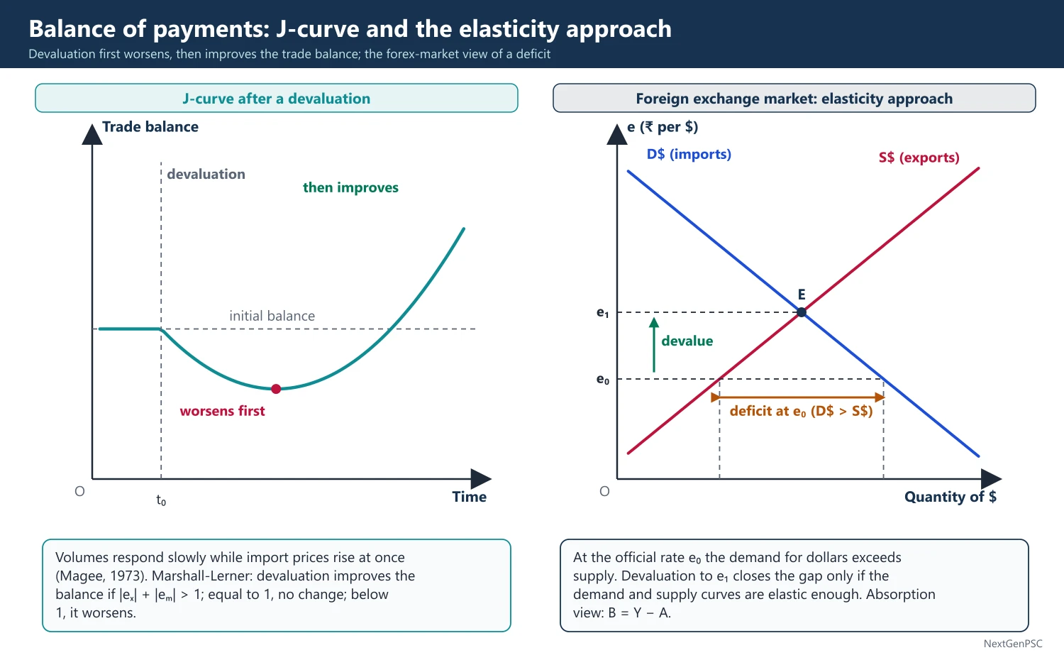
A balance of payments deficit can be corrected through prices or through income. The elasticity approach says a devaluation improves the trade balance only if the Marshall-Lerner condition holds (the sum of import demand elasticities exceeds one), with a J-curve in the short run. Under fixed exchange rates, income adjustment through the foreign trade multiplier corrects only part of a deficit. Alexander's absorption approach (1952) shows that the trade balance improves only if output rises relative to domestic spending (B = Y − A). The monetary approach (Polak, Johnson, Mundell, Frenkel) treats the BoP as a monetary phenomenon: a deficit reflects excess money supply and corrects itself as reserves flow out.
In simple words
A balance of payments deficit means a country is paying more to the world than it earns, like a household spending more than its salary.
The fix can come from making exports cheaper (a weaker rupee), from spending less at home, or from controlling money growth.
Each approach says something different about why a weaker currency sometimes fails to cut the deficit, as India saw before 1991.
UPSC asks you to explain and compare the elasticity, absorption and monetary approaches, with the Marshall-Lerner condition and J-curve.
1. Concepts and Definitions
Balance of payments (BoP): a systematic record of all economic transactions between residents of a country and the rest of the world in a period; it always balances in accounting terms (current account + capital/financial account + errors and omissions + change in reserves = 0).
Current account: trade in goods (merchandise), services, primary income (investment income, wages) and secondary income (remittances, grants).
Capital and financial account: FDI, portfolio investment, loans, banking capital and other flows; in India's presentation, foreign investment, loans, banking capital and rupee debt service.
Deficit or surplus: refers to autonomous (ex ante) transactions; accommodating transactions (reserve changes, IMF borrowing) finance the gap; disequilibrium may be cyclical, secular, structural or fundamental.
Devaluation and depreciation: devaluation is an official cut in a fixed exchange rate; depreciation is a market fall in a floating rate.
2. Automatic Adjustment: Price and Income
Price-specie-flow mechanism: David Hume, 'Of the Balance of Trade' (1752): under the gold standard a deficit causes gold outflow, lowering money supply and prices at home (quantity theory) and raising them abroad, which raises exports and cuts imports until balance is restored.
Income adjustment (Keynesian): a fall in exports reduces income through the foreign trade multiplier k = 1/(s + m), where s is the marginal propensity to save and m the marginal propensity to import; lower income reduces imports.
Incomplete adjustment under fixed rates: if exports rise by ΔX, income rises by ΔX/(s + m) and imports by m·ΔX/(s + m), which is less than ΔX as long as s is positive; so income changes correct only part of a disturbance (Machlup, Metzler).
Foreign repercussions: in a two-country model, a rise in home imports raises foreign income and foreign imports from home, which partly offsets the home deficit; the multiplier with repercussions differs from the simple one.
Price versus income: classical economists relied on price changes (flexible prices and wages); Keynesians showed that with rigid prices, adjustment works through output and employment, which is costly.
3. The Elasticity Approach
Sources: Bickerdike (1920), Joan Robinson (1937) and Lloyd Metzler (1948); Alfred Marshall and Abba Lerner (1944) gave the simple condition.
Assumptions: partial equilibrium, supply elasticities infinite (prices of exports fixed in seller's currency), trade initially balanced, income and other prices constant.
Marshall-Lerner condition: a devaluation improves the trade balance if |eₓ| + |eₘ| is greater than 1, where eₓ is the foreign elasticity of demand for the country's exports and eₘ the home elasticity of demand for imports; if the sum equals 1 the balance is unchanged, if less than 1 it worsens.
General (Bickerdike-Robinson-Metzler) condition: with finite supply elasticities, the condition is less strict; a devaluation can improve the balance even if demand elasticities sum to less than one when supply elasticities are low.
J-curve: in the short run, volumes respond slowly (contracts, habits) while import prices rise at once, so the trade balance first worsens and then improves; first noted by Stephen Magee (1973).
Pass-through: if foreign exporters absorb part of the price change (pricing to market) or domestic exporters raise prices, the effect of devaluation is smaller.
Elasticity pessimism: after World War II many economists doubted that elasticities were high enough (low elasticities in primary products and essential imports such as oil), especially for developing countries.
Criticisms: partial equilibrium; ignores income effects, inflation and capital flows; a devaluation raises domestic prices and may erode its own effect.
4. The Absorption Approach
Source: Sidney Alexander, 'Effects of a Devaluation on a Trade Balance' (IMF Staff Papers, 1952).
Identity: Y = C + I + G + (X − M); define absorption A = C + I + G; then the trade balance B = Y − A.
Implication: a deficit means the country absorbs more than it produces; to improve B, either Y must rise or A must fall: ΔB = ΔY − ΔA.
Decomposition: ΔA = aΔY + ΔD, where a is the propensity to absorb and ΔD the direct effect on absorption; so ΔB = (1 − a)ΔY − ΔD.
Income effects of devaluation: idle resources effect (if there is unemployment, higher net exports raise Y); terms of trade effect (devaluation usually worsens the terms of trade, reducing real income); resource reallocation effect.
Direct absorption effects: real balance effect (higher prices reduce real money balances and spending), money illusion, income redistribution towards profit earners with higher saving propensity, and expectations.
At full employment: Y cannot rise, so devaluation works only if absorption falls; it must be combined with expenditure-reducing (fiscal and monetary tightening) policies.
Contribution and critique: it stresses macro factors ignored by the elasticity approach; Fritz Machlup (1955) criticised its neglect of relative prices; S.C. Tsiang (1961) and others synthesised the two approaches: devaluation (expenditure switching) plus absorption control (expenditure reduction).
5. The Monetary Approach to the Balance of Payments (MABP)
Sources: J.J. Polak (IMF, 1957), Robert Mundell (1968), Harry Johnson (1972), Jacob Frenkel and Johnson, The Monetary Approach to the Balance of Payments (1976).
Core idea: the BoP (overall, including capital) is essentially a monetary phenomenon; a deficit reflects an excess supply of money, a surplus an excess demand for money.
Model: money demand Md = kPY (stable); money supply Ms = m(R + D), with R foreign reserves and D domestic credit; purchasing power parity P = eP*; in equilibrium Md = Ms, so ΔR = ΔMd − ΔD (taking m = 1).
Results: excessive domestic credit creation causes reserve losses; growth in income raises money demand and, without credit expansion, produces a surplus; devaluation raises P and Md and gives only a temporary improvement until money balances adjust.
Under floating rates: the exchange rate, not reserves, adjusts to clear the money market (monetary approach to exchange rates).
Policy: the IMF's financial programming sets ceilings on domestic credit to achieve a reserve target, a practice used in India's 1991 programme.
Criticisms: stable money demand and PPP may not hold in the short run; it ignores the composition of the BoP and real factors; full employment is assumed; sterilisation by central banks breaks the link between reserves and money supply.
6. Diagrams to Draw
J-curve: draw time on the horizontal axis and the trade balance on the vertical; mark devaluation at t0; draw the balance first dipping below its initial level and then rising above it, tracing a J.
Elasticity diagram (foreign exchange market): draw the price of foreign currency (e, rupees per dollar) on the vertical axis and dollars on the horizontal; draw demand for dollars (from imports) and supply of dollars (from exports); at the official rate e0 demand exceeds supply (deficit); a devaluation to e1 closes the gap only if the curves are elastic enough.
Absorption diagram: draw Y on the horizontal axis; draw the 45° line and the absorption line A = A0 + aY with slope less than one; the vertical gap Y − A is the trade balance; devaluation shifts A down (direct absorption) or raises Y (idle resources).
Monetary approach diagram: draw money stock on the horizontal axis and the price level on the vertical; Md slopes up (kPY) and Ms is vertical; if Ms exceeds Md at the PPP price, reserves flow out and Ms shifts left until it equals Md.
7. Examples and Applications
India 1966: the rupee was devalued in June 1966 from ₹4.76 to ₹7.50 per US dollar (a 57.5% rise in the rupee price of the dollar), with weak results because of drought and inelastic exports and imports.
India 1991: foreign exchange reserves fell to about 1 billion US dollars, enough for roughly two weeks of imports; the rupee was devalued in two steps in July 1991 (about 18–19% in total), gold was pledged, an IMF stand-by arrangement was taken, and fiscal and credit restraint cut absorption: a combined elasticity, absorption and monetary programme.
India's current account: the deficit widened to about 2% of GDP in 2022–23 after oil prices rose and narrowed in 2023–24 (RBI), illustrating the role of terms of trade and absorption.
World: the UK devaluation of 1967 and the US dollar depreciation after the Plaza Accord (1985) both showed J-curve patterns.
8. Using it in the Exam
10 marks: state the Marshall-Lerner condition with assumptions and the J-curve.
15 marks: Alexander's absorption approach with B = Y − A and the effects of devaluation on Y and A.
20 marks: compare the three approaches (elasticity, absorption, monetary) with diagrams, their policy implications and India's 1991 experience.
Keywords: autonomous and accommodating transactions, foreign trade multiplier, Marshall-Lerner condition, J-curve, pass-through, absorption, expenditure switching and reducing, domestic credit, PPP, financial programming.
Formula to quote: ΔB = (1 − a)ΔY − ΔD (Alexander, 1952).
| Feature | Elasticity approach | Absorption approach | Monetary approach |
|---|---|---|---|
| Key authors | Marshall, Lerner, Robinson, Metzler | Alexander (1952) | Polak (1957), Johnson, Mundell, Frenkel (1976) |
| Balance analysed | Trade (current) account | Trade (current) account | Overall BoP (reserves) |
| Framework | Partial equilibrium; relative prices | Macro identity B = Y − A | Money market: Md = Ms |
| Condition for devaluation to work | Marshall-Lerner: |eₓ| + |eₘ| greater than 1 | Y must rise relative to A | Only temporary unless domestic credit is restrained |
| Policy stressed | Expenditure switching (devaluation) | Expenditure reduction plus switching | Control of domestic credit |
| Main weakness | Ignores income and money | Neglects relative prices and money | Assumes stable money demand, PPP, full employment |
Mains points
- State the Marshall-Lerner condition exactly, with its assumptions (initially balanced trade, infinite supply elasticities), and add the J-curve.
- Show why income adjustment under fixed rates is incomplete using the foreign trade multiplier.
- Write B = Y − A and ΔB = (1 − a)ΔY − ΔD, and explain idle resources, terms of trade and real balance effects.
- For the monetary approach, write ΔR = ΔMd − ΔD and explain why devaluation has only a temporary effect.
- Conclude with the synthesis: expenditure switching plus expenditure reducing, illustrated by India's 1991 programme.
- Common mistake: applying the Marshall-Lerner condition without stating that it assumes initial trade balance and perfectly elastic supplies.
Did you know?
- Memory trick for the three approaches: 'Prices, Spending, Money' – the elasticity approach looks at prices, the absorption approach at spending (Y − A), and the monetary approach at money (Md − Ms).
Policy Mix: Swan Diagram, Mundell's Assignment and Mundell-Fleming
An open economy seeks internal balance (full employment with price stability) and external balance (a sustainable balance of payments). Meade (1951) showed these can conflict, and Tinbergen (1952) showed two targets need two instruments. The Swan diagram (1955) uses expenditure-changing (absorption) and expenditure-switching (exchange rate) policies to reach both. Mundell (1962) showed that under fixed rates with capital mobility, monetary policy should be assigned to external balance and fiscal policy to internal balance. The Mundell-Fleming model shows that with perfect capital mobility fiscal policy works under fixed rates and monetary policy under floating rates.
In simple words
A country wants two things at once: jobs with low inflation at home (internal balance) and no unsustainable trade deficit abroad (external balance).
It is like steering a car with two controls, the steering wheel and the accelerator: one control cannot handle both direction and speed.
So governments combine budget policy, interest rates and the exchange rate, and the best mix depends on whether the currency floats.
UPSC asks you to draw the Swan diagram, explain Mundell's assignment and state the Mundell-Fleming results.
1. Concepts and Definitions
Internal balance: output at full employment with stable prices.
External balance: a balance of payments position the country regards as sustainable (often current account balance or a target level of reserves).
Meade's conflict: James Meade, The Balance of Payments (1951): with a fixed exchange rate and only demand management, a country with unemployment and a deficit (or inflation and a surplus) faces a dilemma: expanding demand cures unemployment but worsens the deficit.
Tinbergen's rule: Jan Tinbergen, On the Theory of Economic Policy (1952): to reach n independent targets, at least n independent instruments are needed.
Expenditure-changing (reducing) policies: fiscal and monetary policies that change the level of total domestic spending (absorption).
Expenditure-switching policies: policies that shift spending between foreign and domestic goods, mainly exchange rate changes, and also tariffs and export subsidies (Harry Johnson's terminology, 1958).
2. The Swan Diagram Step by Step
Source: Trevor Swan, 'Longer-run Problems of the Balance of Payments' (paper of 1955, published 1963); it formalised Meade's analysis.
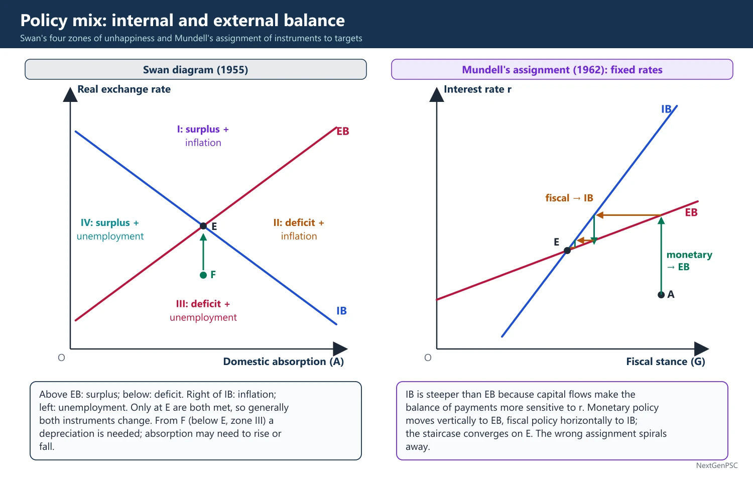
Axes: domestic absorption (real expenditure, A) on the horizontal axis; the real exchange rate (price of foreign currency, a rise meaning depreciation and more competitiveness) on the vertical axis.
External balance (EB) curve: slopes upward: higher absorption raises imports, so a higher (depreciated) exchange rate is needed to keep the current account in balance; points above EB are surplus, points below are deficit.
Internal balance (IB) curve: slopes downward: higher absorption raises demand, so an appreciation (lower exchange rate) is needed to switch demand abroad and avoid inflation; points to the right of IB show inflation, points to the left show unemployment.
Four zones of 'economic unhappiness': north: surplus and inflation; east: deficit and inflation; south: deficit and unemployment; west: surplus and unemployment.
Policy lesson: only at the intersection E are both balances achieved; generally both instruments must change; for example, a point directly below E (deficit with unemployment in the south zone) needs depreciation, and depending on the exact position, absorption may need to rise or fall.
Meade's dilemma cases: unemployment with surplus, or inflation with deficit, can be solved by absorption alone; unemployment with deficit or inflation with surplus need the exchange rate too.
Limitations: it ignores capital flows, assumes the real exchange rate can be controlled (nominal devaluation may be offset by inflation), and treats targets as fixed.
3. Mundell's Assignment Problem
Source: Robert Mundell, 'The Appropriate Use of Monetary and Fiscal Policy for Internal and External Stability' (IMF Staff Papers, 1962).
Setting: fixed exchange rate, capital mobile internationally; instruments: fiscal policy (government spending or budget balance) and monetary policy (interest rate).
Key insight: both policies affect income, but monetary policy also affects capital flows through the interest rate; so monetary policy has a relatively stronger effect on the balance of payments, and fiscal policy on internal balance.
Principle of effective market classification: assign each instrument to the target on which it has the greatest relative effect: monetary policy to external balance, fiscal policy to internal balance.
Stability: with the correct assignment, decentralised policy adjustments converge to the joint equilibrium; with the wrong assignment they spiral away (instability).
Diagram: draw the interest rate on the vertical axis and fiscal stance (government spending or budget deficit) on the horizontal; the IB line slopes up (more spending needs a higher interest rate to keep full employment); the EB line also slopes up but is flatter (a higher interest rate attracts capital, so the BoP is more sensitive to r); show the zig-zag path converging under correct assignment and diverging under wrong assignment.
Criticisms: capital inflows bought with high interest rates are a flow that may not be sustainable; interest payments worsen the current account; capital mobility may be limited; fiscal policy has long lags.
4. The Mundell-Fleming Model
Sources: J. Marcus Fleming, 'Domestic Financial Policies under Fixed and under Floating Exchange Rates' (IMF Staff Papers, 1962), and Robert Mundell, 'Capital Mobility and Stabilization Policy under Fixed and Flexible Exchange Rates' (Canadian Journal of Economics and Political Science, 1963); Mundell received the Nobel Prize in 1999.
Structure: IS-LM extended with a BP curve; IS: Y = C(Y − T) + I(r) + G + NX(e, Y); LM: M/P = L(Y, r); BP: NX(e, Y) + KA(r − r*) = 0.
BP curve slope: upward sloping with imperfect capital mobility (higher Y raises imports, so a higher r is needed to attract capital); horizontal at r = r* with perfect capital mobility; vertical with no capital mobility.
Assumptions: small open economy, fixed prices (short run), static exchange rate expectations, perfect capital mobility in the classic case.
Fixed rates, monetary expansion: LM shifts right, r falls below r*, capital flows out, the central bank sells reserves to defend the rate, money supply falls back: monetary policy is ineffective.
Fixed rates, fiscal expansion: IS shifts right, r tends to rise above r*, capital flows in, the central bank buys foreign exchange, money supply rises (LM shifts right): fiscal policy is highly effective, with no crowding out.
Floating rates, monetary expansion: LM shifts right, r falls, capital flows out, the currency depreciates, net exports rise and IS shifts right: monetary policy is highly effective.
Floating rates, fiscal expansion: IS shifts right, r tends to rise, capital flows in, the currency appreciates, net exports fall and IS shifts back: fiscal policy is ineffective (full crowding out through the trade balance).
Imperfect capital mobility: results depend on whether the BP curve is steeper or flatter than LM; if BP is flatter than LM (high mobility), fiscal expansion causes a BoP surplus under fixed rates and appreciation under floating rates.
Criticisms: fixed prices, static expectations, no wealth or stock effects, small-country assumption; Dornbusch (1976) added sticky prices and rational expectations, producing exchange rate overshooting.
5. Diagrams to Draw
Swan diagram: draw absorption on the horizontal axis and the real exchange rate on the vertical; draw EB sloping up and IB sloping down, crossing at E; label the four zones (I surplus-inflation at the top, II deficit-inflation on the right, III deficit-unemployment at the bottom, IV surplus-unemployment on the left); mark a point in a dilemma zone and show the policy path to E.
Mundell assignment: draw the interest rate against fiscal stance with IB steeper than EB; start at a point off both lines; show monetary policy moving vertically to EB and fiscal policy moving horizontally to IB, converging in a staircase to the intersection.
Mundell-Fleming four panels: in each, draw IS, LM and a horizontal BP at r*; (a) fixed rate, LM shift reverses; (b) fixed rate, IS shift plus induced LM shift raises Y strongly; (c) floating rate, LM shift plus induced IS shift raises Y; (d) floating rate, IS shift reverses through appreciation.
6. Examples and Applications
India: in 1991 India combined devaluation (expenditure switching) with fiscal consolidation and credit restraint (expenditure reducing), a Swan-diagram-type package; under today's managed float and partial capital mobility, the RBI's monetary policy is effective for inflation while fiscal policy faces partial crowding out through the exchange rate.
Hong Kong: with a currency board linked to the US dollar since 1983, Hong Kong cannot use monetary policy; its interest rates follow US rates, a fixed-rate Mundell-Fleming case.
US in the early 1980s: loose fiscal and tight monetary policy under floating rates produced high interest rates, a strong dollar and large trade deficits, as Mundell-Fleming predicts.
Euro area: member countries share a fixed internal exchange rate; fiscal policy is their main national stabilisation tool, consistent with Mundell-Fleming under fixed rates.
7. Using it in the Exam
10 marks: state Tinbergen's rule, Meade's conflict and the two types of policies (expenditure changing and switching).
15 marks: Swan diagram with four zones and policy prescriptions.
20 marks: Mundell's assignment with stability argument and the Mundell-Fleming results under fixed and floating rates with diagrams, applied to India.
Keywords: internal balance, external balance, Tinbergen rule, expenditure switching, expenditure reducing, zones of economic unhappiness, effective market classification, BP curve, perfect capital mobility, policy mix.
Statement to quote: Mundell (1962): monetary policy should be aimed at external objectives and fiscal policy at internal objectives under fixed exchange rates.
| Policy | Fixed exchange rate | Floating exchange rate |
|---|---|---|
| Monetary expansion | Ineffective: reserves flow out, money supply returns to original level | Highly effective: depreciation raises net exports |
| Fiscal expansion | Highly effective: capital inflow expands money supply; no crowding out | Ineffective: appreciation cuts net exports (full crowding out) |
| Mechanism | Central bank intervention changes money supply | Exchange rate adjusts |
| Zone | Condition | Dilemma under absorption alone? | Policy direction |
|---|---|---|---|
| North | Surplus and inflation | Yes | Appreciate; adjust absorption as needed |
| East | Deficit and inflation | No | Reduce absorption (plus exchange rate as needed) |
| South | Deficit and unemployment | Yes | Depreciate; adjust absorption as needed |
| West | Surplus and unemployment | No | Raise absorption (plus exchange rate as needed) |
Mains points
- Start with Tinbergen's rule and Meade's conflict to frame any policy-mix question.
- Draw the Swan diagram with correctly sloped IB (downward) and EB (upward) curves and label all four zones.
- Explain Mundell's assignment using the principle of effective market classification, and show why the wrong assignment is unstable.
- Present Mundell-Fleming results in a 2×2 table and support each cell with the mechanism (reserves or exchange rate).
- Apply to India's managed float with partial capital mobility, and to Hong Kong's currency board as a fixed-rate case.
- Common mistake: reversing the Mundell assignment; under fixed rates monetary policy goes to external balance, fiscal policy to internal balance.
Did you know?
- Memory trick for Mundell-Fleming: 'Fixed loves Fiscal, Floating loves Money' – under fixed rates fiscal policy works, under floating rates monetary policy works.
Exchange Rate Regimes: Fixed, Floating, Currency Boards and Developing Countries
An exchange rate regime is the set of rules by which a country's currency value is determined. Regimes range from hard pegs (currency boards, dollarisation) through soft pegs (adjustable, crawling pegs, bands) and managed floats to free floating. After the gold standard and Bretton Woods (1944–1973), major currencies float. Milton Friedman (1953) argued for flexible rates; critics stress volatility and speculation. A currency board fixes the rate with full reserve backing, giving credibility but no independent monetary policy. For developing countries, floating brings fear of floating (Calvo-Reinhart), original sin (Eichengreen-Hausmann) and pass-through problems, which is why many, including India, run a managed float.
In simple words
The exchange rate is the price of one currency in another, for example how many rupees buy one dollar.
A country can fix that price like a government-set bus fare, or let it float like vegetable prices in a market, or do something in between.
Fixed rates give certainty but can collapse under pressure; floating rates adjust smoothly but can swing wildly, hurting importers and borrowers.
UPSC asks you to compare fixed and floating rates, explain currency boards and judge what suits developing countries like India.
1. Concepts and Definitions
Nominal exchange rate (e): the price of foreign currency in domestic currency (₹ per US dollar); a rise is a depreciation of the rupee.
Real exchange rate: e·P*/P, the relative price of foreign to domestic goods; the real effective exchange rate (REER) is a trade-weighted average against many partners (the RBI publishes 40-currency REER indices).
Purchasing power parity (PPP): Gustav Cassel (1918): absolute PPP, e = P/P*; relative PPP, the percentage change in e equals the inflation differential; holds roughly in the long run, poorly in the short run.
Exchange rate regime: the arrangement for determining the exchange rate; the IMF classifies de facto regimes as hard pegs (no separate legal tender, currency board), soft pegs (conventional peg, stabilised arrangement, crawling peg, crawl-like arrangement, pegged within horizontal bands), floating arrangements (floating, free floating) and other managed arrangements.
2. History of Regimes
Gold standard (about 1870s–1914): currencies convertible into gold at fixed parities; adjustment through the price-specie-flow mechanism; suspended in World War I; restored briefly in the 1920s and abandoned in the 1930s (Britain left in 1931).
Bretton Woods system (1944–1971/73): agreed at the Bretton Woods conference (July 1944), which created the IMF and the World Bank; an adjustable peg: currencies fixed to the US dollar within ±1%, the dollar convertible into gold at 35 US dollars per ounce for central banks; parity changes allowed for 'fundamental disequilibrium'.
Triffin dilemma: Robert Triffin, Gold and the Dollar Crisis (1960): the world needed growing dollar liquidity, which required US deficits, which in turn undermined confidence in dollar-gold convertibility.
Collapse: President Nixon suspended dollar-gold convertibility on 15 August 1971; the Smithsonian Agreement (December 1971) widened bands to ±2.25%; generalised floating began in March 1973; the Jamaica Accords (1976) and the IMF's Second Amendment (1978) legalised floating.
European arrangements: the European Monetary System's Exchange Rate Mechanism (1979) led to the euro (1999).
3. Fixed versus Floating: The Debate
Case for floating: Milton Friedman, 'The Case for Flexible Exchange Rates' (1953): automatic BoP adjustment, monetary policy independence, insulation from foreign inflation and shocks, no need for large reserves, and speculation is stabilising because profitable speculators buy low and sell high.
Case for fixed rates: certainty for trade and investment, discipline on monetary and fiscal policy (a nominal anchor), avoidance of competitive depreciation, and protection against destabilising speculation (Ragnar Nurkse's study of the interwar period, 1944).
Costs of fixed rates: loss of monetary independence with capital mobility (the trilemma), risk of speculative attacks and sudden collapse, need for large reserves.
Costs of floating: volatility and misalignment, exchange rate overshooting (Dornbusch, 1976), inflation pass-through, and balance sheet effects where debts are in foreign currency.
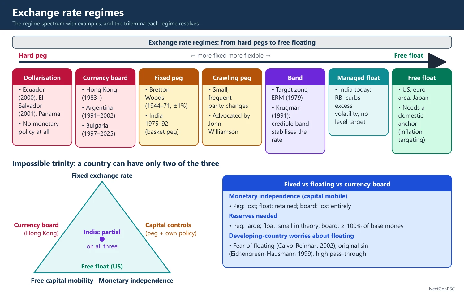
Intermediate regimes: crawling pegs (John Williamson), target zones (Krugman, 1991, showed a credible band stabilises the rate inside it, the 'honeymoon effect'), and managed floats.
Bipolar view: Stanley Fischer (2001) argued that with high capital mobility, soft pegs are crisis-prone, so countries move to hard pegs or floats ('hollowing out of the middle'); later evidence shows many countries still use intermediate regimes.
4. Currency Boards
Definition: a monetary arrangement with a legislated commitment to exchange domestic currency for a specified foreign currency at a fixed rate, with base money fully (100% or more) backed by foreign reserves.
Features: no discretionary monetary policy; money supply changes only with reserves; the central bank cannot act as an unlimited lender of last resort or finance the government.
Benefits: strong credibility, rapid disinflation, low interest rates if trusted; useful after hyperinflation or for small open economies.
Costs: no independent monetary policy or exchange rate adjustment; vulnerability to asymmetric shocks and real appreciation; banking crises cannot be met by money creation; exit is costly.
Examples: Hong Kong (since October 1983, about HK 7.8 per US dollar, with a band of 7.75–7.85 since 2005); Argentina's Convertibility Plan (1991–2002, one peso per dollar), which ended in crisis, default and devaluation in January 2002; Estonia (1992–2010, then euro); Lithuania (1994–2014, then euro); Bulgaria (1997 until it adopted the euro on 1 January 2026); Bosnia and Herzegovina (from 1997).
Lesson from Argentina: a currency board cannot survive persistent fiscal deficits, a strong dollar and an overvalued real exchange rate; it needs fiscal discipline and flexible wages.
5. Floating Rates and Developing Countries
Fear of floating: Guillermo Calvo and Carmen Reinhart (2002) found that many countries that declare floating actually intervene heavily, because of pass-through to inflation, foreign currency debt and lack of credibility.
Original sin: Barry Eichengreen and Ricardo Hausmann (1999): most developing countries cannot borrow abroad in their own currency, so depreciation raises the burden of debt (currency mismatch), turning depreciation contractionary.
High pass-through: depreciation quickly raises domestic prices of imported fuel and food, threatening inflation targets.
Thin markets and volatility: shallow foreign exchange markets and volatile capital flows cause large swings; reserves are needed as self-insurance.
Policy responses: managed floats with intervention against excess volatility, reserve accumulation, inflation targeting as the nominal anchor, macroprudential and capital flow measures (endorsed by the IMF's Institutional View, 2012), and developing local currency bond markets.
Dollarisation: Ecuador (2000), El Salvador (2001) and Panama use the US dollar, giving up monetary policy entirely.
6. India's Exchange Rate Regime
Evolution: par value under Bretton Woods (1947–1971); peg to the pound sterling (1971–1975); peg to a basket of currencies (September 1975–1992); devaluations of June 1966 and July 1991.
Liberalised Exchange Rate Management System (LERMS, March 1992): a dual rate: 60% of export earnings converted at the market rate and 40% at the official rate; replaced by a unified, market-determined rate in March 1993.
Convertibility: current account convertibility from August 1994 (acceptance of IMF Article VIII); capital account liberalised gradually following the Tarapore Committees (1997 and 2006).
Present regime: a managed float: the RBI intervenes in spot, forward and swap markets to curb excess volatility without targeting a level; reserves reached a peak of about 705 billion US dollars in September 2024.
IMF classification: the IMF reclassified India's de facto regime as a 'stabilised arrangement' for December 2022 to October 2023, a view the RBI disagreed with; India officially describes its regime as market-determined.
7. Diagrams to Draw
Foreign exchange market under floating: draw the price of dollars (₹ per US dollar) on the vertical axis and the quantity of dollars on the horizontal; draw demand for dollars (imports, capital outflows) sloping down and supply (exports, inflows) sloping up; a rise in demand raises e from e0 to e1 (depreciation).
Fixed rate defence: at the fixed rate ē below the market equilibrium, show excess demand for dollars; the central bank sells reserves equal to the gap; under a currency board, money supply contracts by the same amount.
Regime spectrum: draw a horizontal line from 'hard peg' (left) to 'free float' (right) with currency board, conventional peg, crawling peg, band, managed float and free float marked, and examples beneath each.
Impossible trinity triangle: show which side each regime occupies (currency board: fixed rate plus free capital; India: partial on all three).
8. Using it in the Exam
10 marks: currency board: features, merits, demerits and one example (Hong Kong or Argentina).
15 marks: fixed versus floating with Friedman's case and the critics.
20 marks: implications of floating for developing countries (fear of floating, original sin, pass-through), intermediate regimes and India's managed float with its evolution since 1991.
Keywords: PPP, REER, adjustable peg, Triffin dilemma, managed float, crawling peg, currency board, bipolar view, fear of floating, original sin, dollarisation, LERMS.
Statement to quote: Calvo and Reinhart (2002) found that many emerging economies that claim to float in fact limit exchange rate movements, a behaviour they called fear of floating.
| Feature | Fixed (adjustable) peg | Free float | Currency board |
|---|---|---|---|
| Monetary policy independence (with capital mobility) | Lost | Retained | Lost entirely |
| BoP adjustment | Through reserves and income; occasional devaluation | Through exchange rate | Through money supply, prices and income |
| Credibility / anchor | Moderate; speculative attacks possible | Needs domestic anchor (inflation targeting) | High if fiscally disciplined |
| Reserves needed | Large | Small in theory | At least 100% of base money |
| Examples | Bretton Woods (1944–71); India 1975–92 basket peg | US, euro area vis-à-vis others, Japan | Hong Kong (1983–), Argentina (1991–2002), Bulgaria (1997–2025) |
Mains points
- Start with the spectrum of regimes (IMF de facto classification) and the trilemma, then compare fixed and floating with arguments on both sides.
- For currency boards, give the 100% backing rule, the loss of lender-of-last-resort function, and contrast Hong Kong's survival with Argentina's collapse.
- For developing countries, use fear of floating (Calvo-Reinhart), original sin (Eichengreen-Hausmann) and pass-through to explain managed floats.
- Trace India's regime: basket peg (1975), 1991 devaluation, LERMS (1992), unified rate (1993), current account convertibility (1994), managed float now.
- Mention Friedman's stabilising speculation argument and Nurkse's interwar counter-evidence.
- Common mistake: calling India's regime a free float; it is a managed float with intervention against volatility.
Did you know?
- Hong Kong's currency board was set up in October 1983 during a panic over the territory's future, when the Hong Kong dollar had fallen sharply; the link at about 7.8 to the US dollar has survived every crisis since, including 1997–98.
Capital Mobility, Speculation and International Policy Coordination
With high capital mobility, exchange rates are set mainly in asset markets: interest parity links interest differentials to expected or forward exchange rate changes, and Dornbusch (1976) showed that sticky goods prices make exchange rates overshoot after monetary shocks. Speculation can stabilise (Friedman, 1953) or destabilise (Nurkse, 1944); currency crisis models explain attacks on pegs by weak fundamentals (Krugman, 1979), self-fulfilling expectations (Obstfeld) or financial fragility (Asian crisis, 1997). Because policies spill across borders, international policy coordination (Hamada's game theory, the Plaza and Louvre Accords, the G20 in 2008–09) can raise welfare, but it is hard to sustain.
In simple words
Today trillions of dollars move between countries every day in search of higher returns; this is capital mobility.
Like water flowing to the lowest point, money flows to where interest rates are higher, pushing that currency up, and can rush out just as fast in a panic.
Speculators betting on a currency fall can break a fixed rate, as in Britain in 1992 and East Asia in 1997, so countries sometimes act together.
UPSC asks about speculation, currency crises, exchange rate adjustment under capital mobility and the need for policy coordination.
1. Concepts and Definitions
Capital mobility: the ease with which financial capital moves between countries; perfect mobility means domestic and foreign assets are perfect substitutes and any interest differential (adjusted for expected exchange rate change) is eliminated at once.
Covered interest parity (CIP): i − i* = (F − S)/S, where S is the spot rate, F the forward rate (domestic currency per foreign unit), i and i* the domestic and foreign interest rates; arbitrage keeps it close to holding in liquid markets.
Uncovered interest parity (UIP): i − i* = expected rate of depreciation of the domestic currency; empirically violated in the short run (the forward premium puzzle, Fama, 1984), which makes 'carry trades' profitable on average but risky.
Speculation: buying or selling foreign exchange in the expectation of profit from future rate changes; 'hot money' refers to short-term, highly mobile capital flows.
Policy coordination: joint adjustment of national macroeconomic policies to take account of spillovers between countries.
2. Exchange Rate Adjustment under Capital Mobility
Asset market view: with high capital mobility, the exchange rate is determined by the demand and supply of stocks of financial assets, not by trade flows; it moves quickly and responds to news and expectations.
Monetary approach to exchange rates: Frenkel (1976) and others: with flexible prices and PPP, e = M/(kY) divided by M*/(k*Y*); a rise in domestic money supply causes a proportionate depreciation.
Portfolio balance approach: William Branson and others: domestic and foreign bonds are imperfect substitutes, so the exchange rate also depends on relative asset supplies and risk premiums; sterilised intervention can then affect the rate.
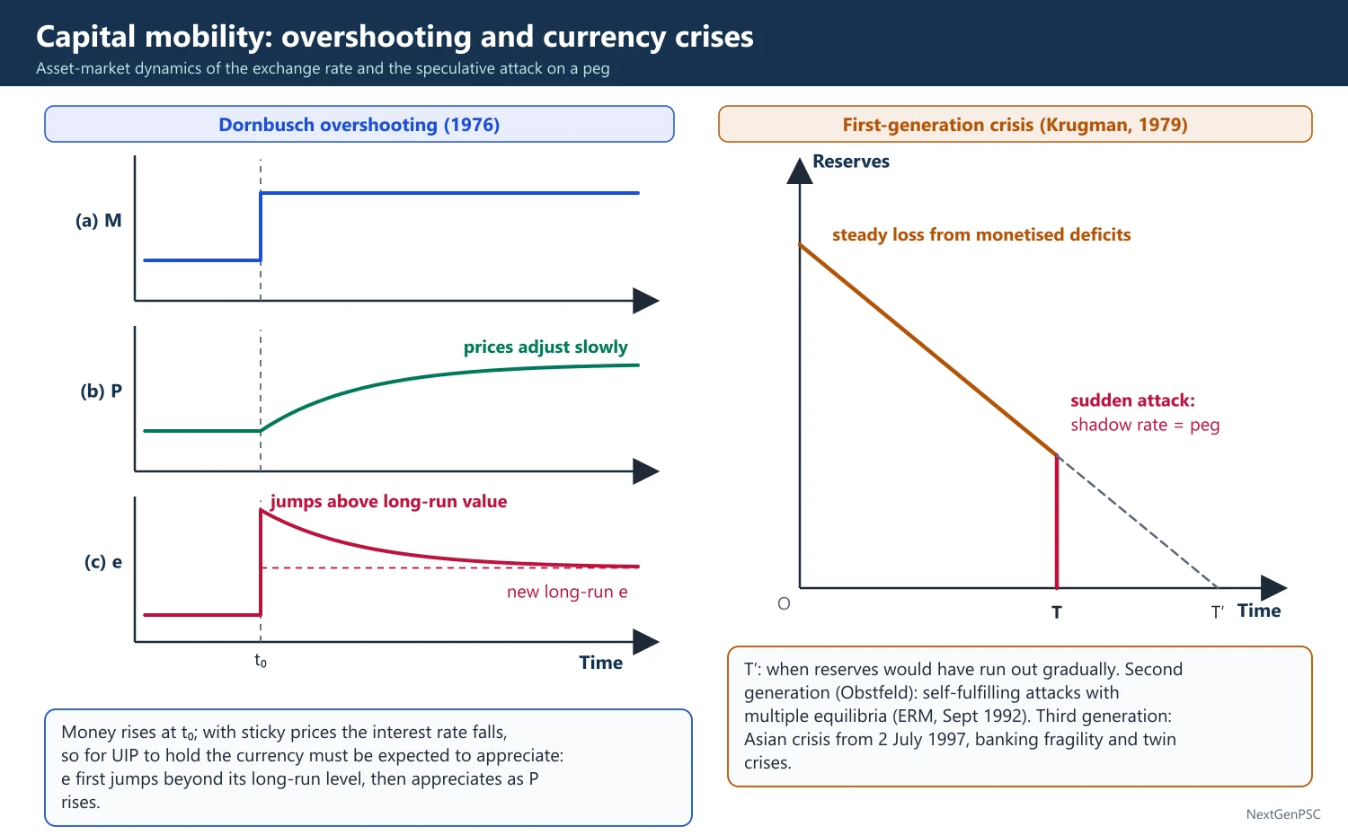
Dornbusch overshooting: Rudiger Dornbusch, 'Expectations and Exchange Rate Dynamics' (Journal of Political Economy, 1976): goods prices are sticky, asset markets clear instantly and UIP holds; a monetary expansion lowers the domestic interest rate; for UIP to hold the currency must be expected to appreciate, which is possible only if it first depreciates beyond its long-run level; it then appreciates gradually as prices rise.
Significance: overshooting explains why floating rates are more volatile than fundamentals such as prices and output, without assuming irrational speculation.
Mundell-Fleming link: under perfect capital mobility, monetary policy affects output through the exchange rate (floating) and fiscal policy through money supply changes (fixed), as covered under policy mix.
3. Speculation: Stabilising or Destabilising?
Friedman's argument (1953): profitable speculation means buying when the currency is cheap and selling when it is dear, which smooths fluctuations; destabilising speculators lose money and are driven out.
Nurkse's counter-evidence (1944): Ragnar Nurkse's League of Nations study of the interwar period found that speculation often aggravated currency instability (France in the 1920s).
Bandwagon effects and herding: extrapolative expectations, Keynes' 'beauty contest' (General Theory, 1936, chapter 12) where traders guess what others will think, and rational bubbles can make speculation destabilising.
Chartists and fundamentalists: Frankel and Froot (1990) showed how the mix of trend-following chartists and fundamentalists can cause swings away from fundamentals (the 1980s dollar).
4. Currency Crisis Models
First generation: Paul Krugman, 'A Model of Balance-of-Payments Crises' (Journal of Money, Credit and Banking, 1979), based on Salant and Henderson (1978): a government that monetises fiscal deficits under a peg steadily loses reserves; speculators attack when the 'shadow' floating rate equals the peg, exhausting reserves in one sudden attack; the crisis is caused by inconsistent fundamentals (Mexico 1982, Argentina 1981).
Second generation: Maurice Obstfeld (1986, 1994): the government weighs the costs of defending the peg (high interest rates, unemployment) against its benefits; if markets expect devaluation, defence becomes costlier, so expectations can be self-fulfilling and multiple equilibria exist; example: the ERM crisis of September 1992, when the UK left the ERM on 16 September ('Black Wednesday') after attacks by speculators including George Soros.
Third generation: the Asian crisis (from the Thai baht's float on 2 July 1997) involved banking fragility, moral hazard from implicit guarantees (Krugman, 1998; Corsetti, Pesenti and Roubini), balance sheet effects from foreign currency debt and 'twin crises' of banks and currencies (Kaminsky and Reinhart, 1999).
Sudden stops: Guillermo Calvo (1998): an abrupt halt of capital inflows forces a sharp current account adjustment and output collapse.
Contagion: crises spread through trade links, common lenders and investor panic (Russia 1998, Brazil 1999).
5. Managing Capital Flows and Speculation
Tobin tax: James Tobin proposed (1972 lectures; 'A Proposal for International Monetary Reform', 1978) a small uniform tax on currency transactions to 'throw some sand in the wheels' of short-term speculation while barely affecting long-term trade and investment.
Capital controls: Chile's unremunerated reserve requirement on inflows (1991–98) and Malaysia's outflow controls (September 1998) are cited as cases where controls helped manage flows (debated); the IMF's Institutional View (2012) accepts capital flow management measures in some circumstances.
Reserves and swap lines: large reserves, regional arrangements (the Chiang Mai Initiative, 2000) and central bank swap lines (US Federal Reserve swap lines in 2008 and 2020) act as insurance.
Sequencing: liberalise the capital account only after fiscal consolidation, low inflation and a sound financial sector (McKinnon; India's Tarapore Committees of 1997 and 2006 set such preconditions).
6. International Policy Coordination
Why coordinate: in interdependent economies, one country's fiscal or monetary policy affects others through trade, interest rates and exchange rates; uncoordinated (Nash) policies may be inefficient, as each ignores spillovers.
Hamada's analysis: Koichi Hamada (1976; The Political Economy of International Monetary Interdependence, 1985) used game theory to show that cooperative (Pareto-efficient) policies give higher welfare than the non-cooperative Nash equilibrium.
Locomotive theory: at the Bonn summit (1978) Germany and Japan agreed to expand demand to pull the world economy, an early coordination attempt.
Plaza Accord (September 1985): the G5 (US, Japan, West Germany, France, UK) agreed to intervene to depreciate the overvalued US dollar.
Louvre Accord (February 1987): the major economies agreed to stabilise exchange rates around current levels after the dollar's fall.
G20 response to the 2008 crisis: the G20 leaders' summits from November 2008 (Washington) and April 2009 (London) coordinated fiscal stimulus, expanded IMF resources and agreed financial regulatory reform; the G20 Mutual Assessment Process (2009) reviews policy consistency.
Obstacles: disagreement over the correct economic model (Frankel and Rockett, 1988, showed coordination based on the wrong model can lower welfare); free riding and credibility problems; domestic political constraints; Rogoff (1985) showed that coordination among central banks can be counterproductive if it weakens their anti-inflation credibility.
Current issues: spillovers from US monetary policy to emerging markets (taper tantrum 2013; the 2022 tightening), 'currency wars' (a term used by Brazil's finance minister Guido Mantega in 2010), and calls by India and other emerging economies in the G20 for central banks in advanced economies to consider spillovers.
7. Diagrams to Draw
Dornbusch overshooting: draw time on the horizontal axis; in three stacked panels show (a) money supply jumping up at t0, (b) the price level rising gradually to its new level, (c) the exchange rate jumping at t0 above its new long-run value and then declining gradually to it.
UIP diagram: draw the exchange rate on the vertical axis and expected returns on the horizontal; the domestic deposit return is a vertical line at i; the expected return on foreign deposits slopes down with e; equilibrium is where they intersect; a fall in i shifts the vertical line left and raises e (depreciation).
First-generation crisis: draw time on the horizontal axis and reserves on the vertical; reserves decline steadily from monetised deficits and then drop to zero in a sudden attack at time T before they would have run out gradually.
Coordination game: draw a 2×2 payoff matrix for two countries choosing expand or restrain; show the Nash equilibrium (both restrain) and the cooperative outcome (both expand) with higher payoffs.
8. Examples and Applications
India: the 1991 crisis was a mix of first-generation (fiscal deficits) and confidence factors (NRI deposit withdrawal after the Gulf war oil shock); in the 2013 taper tantrum the rupee fell to about 68 per US dollar in August 2013, and the RBI used rate measures, a special swap window for oil companies and FCNR(B) deposit schemes; India's reserves and gradual capital account opening helped it avoid the 1997 Asian crisis.
UK 1992: Black Wednesday, a second-generation case.
East Asia 1997–98: Thailand, Indonesia and South Korea, a third-generation case leading to IMF programmes.
Global 2008–09: G20 coordination and Federal Reserve swap lines stabilised markets.
9. Using it in the Exam
10 marks: stabilising versus destabilising speculation (Friedman versus Nurkse) or the Tobin tax.
15 marks: exchange rate adjustment under capital mobility: interest parity and Dornbusch overshooting with diagram.
20 marks: currency crisis models (three generations) with examples, management of capital flows, and the case for and obstacles to international policy coordination, with India's experience.
Keywords: capital mobility, CIP, UIP, asset market approach, overshooting, hot money, speculative attack, self-fulfilling crisis, twin crises, sudden stop, Tobin tax, capital controls, Nash versus cooperative equilibrium, Plaza Accord.
Quotation: Tobin's aim for his currency transactions tax was to 'throw some sand in the wheels' of international finance.
| Generation | Key authors | Cause of crisis | Example |
|---|---|---|---|
| First | Krugman (1979); Flood-Garber (1984) | Fiscal deficits monetised under a peg; steady reserve loss; predictable attack | Mexico 1982; Argentina 1981 |
| Second | Obstfeld (1986, 1994) | Government weighs cost of defence; self-fulfilling expectations; multiple equilibria | ERM crisis 1992 (UK, Italy) |
| Third | Krugman (1998); Corsetti-Pesenti-Roubini; Kaminsky-Reinhart (1999) | Banking fragility, moral hazard, foreign currency debt; twin crises | Asian crisis 1997–98 |
| Sudden stop | Calvo (1998) | Abrupt halt of capital inflows | Mexico 1994–95; Argentina 2001 |
Mains points
- Explain exchange rate determination under capital mobility with CIP and UIP, then Dornbusch overshooting with its three-panel diagram.
- Present the speculation debate as Friedman (stabilising) versus Nurkse and Keynes (destabilising), with modern evidence on herding.
- Classify currency crises into generations with authors and examples; a table scores well.
- Discuss tools to manage flows: reserves, capital flow measures (IMF Institutional View 2012), Tobin tax, swap lines.
- For coordination, use Hamada's game theory, the Plaza (1985) and Louvre (1987) accords and the G20 (2008–09), then list obstacles (model uncertainty, free riding, Rogoff's critique).
- Common mistake: treating all currency crises as caused by bad fundamentals; second-generation models show self-fulfilling attacks can hit sound economies.
Did you know?
- George Soros's fund is widely reported to have made about one billion pounds by betting against sterling before the UK left the ERM on 16 September 1992, earning him the label 'the man who broke the Bank of England'.
UPSC Previous Year Questions: Balance of Payments and Exchange Rates
From 2014 to 2026 UPSC asked 28 question parts (405 marks) from Balance of Payments and Exchange Rates. BoP adjustment (elasticity, absorption and monetary approaches, J-curve, foreign trade multiplier: 9 parts) and the Mundell-Fleming policy mix (8 parts) dominate, followed by exchange rate regimes and capital mobility, speculation and policy coordination. Every question below has a model answer written to the UPSC word limit.
In simple words
Read the question and spend five minutes writing your own outline: the approach or model, its condition (Marshall-Lerner, BP slope), the diagram and the conclusion.
Then read the model answer and tick what you missed: the IS-LM-BP shifts, the exchange-rate regime, the Indian example (RBI intervention, rupee, oil).
Practise the Mundell-Fleming and Swan diagrams until you can draw them in two minutes, then rewrite one answer a day within the word limit.
1. Balance of Payments Adjustment: Elasticity, Absorption and Monetary Approaches
Example 1 (UPSC 2025, 10 marks): What is J-curve effect? Explain it graphically.
Paper and question: Paper I, Q5(b)
Approach: Define the J-curve, explain why the trade balance first worsens and then improves after depreciation (short-run inelasticity, contracts, lags), and draw it.
The J-curve effect describes the time path of a country's trade balance after a depreciation or devaluation: it first worsens and only later improves, tracing a J shape.
Reasons: immediately after depreciation, import and export quantities are fixed by existing contracts and habits, so in the short run demand is inelastic and the Marshall-Lerner condition does not hold. The domestic-currency cost of imports rises at once, while export volumes respond slowly, so the trade balance in domestic currency deteriorates. Over time, as contracts expire, buyers switch to cheaper home goods, and exporters expand capacity and markets, elasticities rise; once the sum of the import demand elasticities exceeds one, the trade balance improves.
Diagram: time on the horizontal axis and the trade balance on the vertical; at the moment of depreciation the curve dips below its initial level, reaches a trough, then rises above the initial level, like the letter J.
Example: the US trade deficit kept widening for about two years after the dollar's depreciation following the Plaza Accord (1985). The J-curve warns that the benefits of depreciation take time and that short-run deterioration should not be mistaken for failure.
Example 2 (UPSC 2024, 20 marks): Discuss the elasticity approach and absorption approach for adjustments in balance of payments.
Paper and question: Paper I, Q6(a)
Approach: Explain the elasticity approach (Marshall-Lerner condition, J-curve) and the absorption approach (Alexander's B = Y − A, income and absorption effects), compare them and show they are complementary.
Both approaches analyse how a devaluation (or depreciation) can correct a current account deficit, but they emphasise different mechanisms.
Elasticity approach (Marshall, Lerner, Joan Robinson): devaluation changes relative prices, making exports cheaper abroad and imports dearer at home. Whether the trade balance improves depends on demand elasticities. The Marshall-Lerner condition states that, starting from balanced trade and with infinitely elastic supplies, devaluation improves the trade balance if the sum of the absolute price elasticities of demand for exports and imports exceeds one (|ex| + |em| greater than 1). In the short run elasticities are low, giving the J-curve.
Absorption approach (Sidney Alexander, 1952): from national income accounting, B = Y − A, where A = C + I + G is domestic absorption. A deficit means the country spends more than it produces, so devaluation can improve B only if it raises output Y relative to absorption or reduces absorption. ΔB = (1 − a)ΔY − ΔAd, where a is the propensity to absorb and ΔAd the direct effect on absorption. With unemployment, devaluation raises Y through net exports (income effect); at full employment it must reduce absorption through the real balance effect, money illusion, redistribution towards high savers or higher taxes, otherwise it only causes inflation.
Comparison: the elasticity approach focuses on relative prices (expenditure switching), the absorption approach on aggregate spending and output (expenditure reduction); the first is micro and partial, the second macro and general. Alexander first presented them as rivals, but Machlup and later writers showed they are complementary: devaluation needs favourable elasticities to switch spending, and absorption must fall relative to income to make room for better net exports.
Hence, as in India's 1991 adjustment, devaluation was combined with fiscal consolidation to reduce absorption.
Example 3 (UPSC 2024, 15 marks): Explain how the elasticity of demand for foreign exchange is influenced by the elasticity of home demand for imports and by the elasticity of home supply of import-competing goods.
Paper and question: Paper I, Q6(c)
Approach: Derive the elasticity of import demand from home demand and supply (eM = eD·D/M + eS·S/M), link it to the elasticity of demand for foreign exchange, and explain with a diagram and example.
A country's demand for foreign exchange arises from its imports: the quantity of foreign currency demanded equals the foreign-currency price of imports times the volume of imports. With foreign-currency prices given, a rise in the exchange rate (depreciation) raises the domestic price of imports and reduces the volume imported in proportion to the elasticity of import demand; so the elasticity of demand for foreign exchange equals the elasticity of import demand.
Import demand is excess demand: imports M = D − S, where D is home demand and S is home supply of the import-competing good. When the domestic price rises by a small percentage, D falls and S rises, so imports fall by both amounts. Hence eM = eD × (D/M) + eS × (S/M), where eD is the (absolute) elasticity of home demand and eS the elasticity of home supply of import-competing goods.
Implications: (i) the more elastic home demand, the more imports fall; (ii) the more elastic home supply of import substitutes, the more domestic producers replace imports; (iii) because D/M and S/M exceed one when imports are a small share of consumption, import demand is more elastic than either home demand or supply.
Diagram: home demand and supply of the importable; import demand derived as the horizontal gap between them, flatter than either curve; the resulting demand curve for foreign exchange slopes down with that elasticity.
So a country with good domestic substitutes and price-sensitive consumers has an elastic demand for foreign exchange, which makes depreciation effective; a country dependent on essential imports such as crude oil (India) has an inelastic demand.
Example 4 (UPSC 2023, 20 marks): Explain the concept of "sterilization" in the context of monetary approach to balance of payments.
Paper and question: Paper I, Q4(a)
Approach: Set out the monetary approach (money supply H = D + R, BoP as a monetary phenomenon, automatic adjustment), define sterilisation and show how it blocks adjustment, with India's experience (MSS 2004) and limits.
The monetary approach to the balance of payments (Harry Johnson, Robert Mundell, Jacob Frenkel, 1970s) treats the BoP as a monetary phenomenon: a surplus or deficit reflects an imbalance between the demand for and the supply of money. The monetary base is H = D + R, where D is domestic credit of the central bank and R is foreign exchange reserves.
Automatic adjustment under fixed rates: if domestic credit expands faster than money demand, people spend the excess money on foreign goods and assets, creating a BoP deficit. The central bank sells reserves to defend the peg, so R and the money supply fall until money supply again equals money demand and the deficit disappears. The BoP is thus self-correcting: ΔR = ΔMd − ΔD.
Sterilisation is the action of the central bank to offset the effect of reserve changes on the monetary base. With a surplus, reserves rise and the bank sells government securities (open market operations) to reduce domestic credit by the same amount, so H stays unchanged; with a deficit, it buys securities to replace the lost reserves.
Consequence: sterilisation blocks the automatic adjustment mechanism: the money supply does not change, so the imbalance persists and reserves keep changing.
India: during the large capital inflows of 2003–08 the RBI bought dollars and sterilised through open market sales and the Market Stabilisation Scheme (introduced in 2004), under which government securities were issued to absorb liquidity. The costs were the interest on these securities, and upward pressure on domestic interest rates, which attracts more inflows.
Hence sterilisation lets a central bank control domestic money and inflation in the short run, but it cannot prevent the adjustment that the monetary approach predicts in the long run.
Example 5 (UPSC 2018, 10 marks): Under what conditions will devaluation create trade surplus and increase output in the simple Keynesian framework?
Paper and question: Paper I, Q5(a)
Approach: In the Keynesian open-economy model, state the conditions: the Marshall-Lerner condition for a trade improvement, idle resources and price rigidity for output to rise, and that the multiplier-induced import rise is smaller than the initial improvement.
In the simple Keynesian open-economy model, Y = C + I + G + X − M, with M = mY, prices fixed and unemployed resources. A devaluation affects output through net exports.
Conditions: (i) the Marshall-Lerner condition: the sum of the absolute price elasticities of demand for exports and imports must exceed one (starting from balanced trade), so that devaluation raises net exports at the initial income; (ii) unemployed resources and rigid money wages and prices, so that higher demand raises real output rather than prices; (iii) a positive marginal propensity to save, so that the multiplier 1/(s + m) is finite. Output then rises by ΔY = ΔNX₀/(s + m).
Because part of the extra income is spent on imports (mΔY), the final improvement in the trade balance is ΔNX₀ × s/(s + m), smaller than the initial improvement but still positive as long as s is positive.
If the economy is at full employment, or devaluation raises domestic prices and wages, the gains are eroded.
Example 6 (UPSC 2017, 15 marks): "Monetary Contraction is a better option than devaluation to improve balance of payments position of a developing economy under fixed exchange rate system." Discuss.
Paper and question: Paper I, Q6(b)
Approach: Compare expenditure-reducing (monetary contraction) and expenditure-switching (devaluation) policies for a developing economy under a fixed rate, using the absorption and monetary approaches and the Swan logic; give a balanced view.
Under a fixed exchange rate, a BoP deficit can be corrected by expenditure reduction (monetary or fiscal contraction) or expenditure switching (devaluation). The statement favours the first.
For monetary contraction: in the monetary approach a deficit reflects excess money supply, so cutting domestic credit attacks the root cause; it lowers absorption and imports, raises interest rates and attracts capital; it avoids the inflationary pass-through of devaluation, which is strong in developing countries dependent on oil, fertiliser and capital goods imports; and it avoids the loss of credibility of a peg. Where export and import elasticities are low (export pessimism, J-curve), devaluation may not even improve the trade balance.
Against: monetary contraction works by reducing income and employment; in a developing economy with unemployment and weak transmission, the output cost per unit of BoP improvement is high, and higher interest rates hurt investment and growth. If the deficit stems from an overvalued currency (a real misalignment), only switching corrects relative prices; contraction then causes prolonged recession. The Swan diagram shows that with two targets, internal and external balance, two instruments are needed (Tinbergen).
Hence monetary contraction is better when the deficit comes from excess demand or credit, as in many IMF programmes; devaluation is needed when the real exchange rate is overvalued. Usually a combination works best, as in India's 1991 programme of devaluation plus fiscal and monetary tightening.
Example 7 (UPSC 2016, 20 marks): What are the elasticity and absorption approaches to BOP adjustment? Discuss.
Paper and question: Paper I, Q8(a)
Approach: Explain the elasticity approach (Marshall-Lerner, J-curve, limitations) and the absorption approach (B = Y − A, income and absorption effects at less than and at full employment), then their synthesis.
The elasticity approach analyses how a devaluation improves the trade balance through relative price changes. Devaluation lowers the foreign-currency price of exports and raises the domestic-currency price of imports. By the Marshall-Lerner condition, starting from balanced trade with perfectly elastic supplies, the trade balance improves if |ex| + |em| is greater than one; the more general Bickerdike-Robinson-Metzler condition allows for finite supply elasticities.
Diagram: foreign-exchange market with demand (from imports) and supply (from exports) curves; devaluation raises the price of foreign currency; if demand and supply are elastic the gap between them (the deficit) narrows; with inelastic, backward-bending supply it may widen. A time diagram shows the J-curve, since elasticities are low in the short run.
Limitations: it is partial equilibrium, ignores the effect of devaluation on income, absorption and domestic prices, and assumes unemployed resources. Developing countries' elasticities may be low.
The absorption approach (Sidney Alexander, 1952) starts from B = Y − A, where absorption A = C + I + G. The trade balance improves only if income rises relative to absorption: ΔB = (1 − a)ΔY − ΔAd. With unemployment, devaluation raises net exports and income (the income or employment effect), and B improves if the propensity to absorb is below one. At full employment Y cannot rise, so devaluation must reduce absorption directly, through the real-balance effect (higher prices reduce real money holdings), redistribution towards profits and high savers, money illusion or higher taxes; otherwise it merely causes inflation.
Synthesis: the two approaches are complementary (Machlup; Tsiang): devaluation switches expenditure if elasticities are favourable, but sustained improvement requires that absorption falls relative to output, which is why devaluation is usually accompanied by expenditure-reducing fiscal and monetary policies.
Example 8 (UPSC 2015, 10 marks): How do depreciation and appreciation in the external value of a currency impact a country's balance of payments?
Paper and question: Paper I, Q5(d)
Approach: Explain how depreciation and appreciation affect the current account (Marshall-Lerner, J-curve), the capital account (expectations, valuation) and reserves, with India's example.
Depreciation (a fall in the external value of the currency) makes exports cheaper for foreigners and imports dearer at home. If the Marshall-Lerner condition holds (sum of export and import demand elasticities greater than one), the trade balance improves, though after a lag (the J-curve). It also raises the domestic-currency value of remittances and income from abroad, but increases the burden of foreign-currency debt and can be inflationary, eroding the gain.
Appreciation has the opposite effects: exports lose competitiveness and imports become cheaper, so the trade balance tends to worsen, though cheaper imported inputs and lower inflation help.
On the capital account, expected further depreciation can trigger outflows, while a depreciation seen as complete can attract inflows.
India's rupee depreciation in 2013 widened the oil import bill at first, showing the J-curve, while services exports benefited.
Example 9 (UPSC 2015, 20 marks): In the context of a two-country model, derive foreign trade multiplier and explain its working. What will be its repercussion?
Paper and question: Paper I, Q6(a)
Approach: Derive the open-economy multiplier without repercussion, then the two-country multiplier with foreign repercussion step by step, interpret it with a numerical illustration and explain the repercussion effects and limitations.
The foreign trade multiplier (Harrod, Machlup) shows how a change in autonomous spending changes national income when part of extra income leaks into imports. With imports M = mY, the small-country multiplier is k = 1/(s + m), smaller than the closed-economy 1/s.
Two-country model: countries 1 and 2 with saving propensities s₁, s₂ and import propensities m₁, m₂; country 1's exports are country 2's imports. Equilibrium: (s₁ + m₁)Y₁ = A₁ + m₂Y₂ and (s₂ + m₂)Y₂ = A₂ + m₁Y₁, where A is autonomous spending.
Step 1: let autonomous investment in country 1 rise by ΔA₁. From the second equation, ΔY₂ = m₁ΔY₁/(s₂ + m₂).
Step 2: substituting, (s₁ + m₁)ΔY₁ − m₂m₁ΔY₁/(s₂ + m₂) = ΔA₁, so ΔY₁/ΔA₁ = (s₂ + m₂)/(s₁s₂ + s₁m₂ + s₂m₁).
Step 3 (illustration): with s₁ = s₂ = 0.2, m₁ = 0.2 and m₂ = 0.1, the simple multiplier is 1/(0.2 + 0.2) = 2.5, while the multiplier with repercussion is 0.3/(0.04 + 0.02 + 0.04) = 0.3/0.10 = 3.
Working and repercussion: higher investment in country 1 raises its income; part leaks into imports from country 2, raising country 2's exports and income; country 2 then imports more from country 1, which feeds back into country 1's income. This foreign repercussion makes the multiplier larger than 1/(s₁ + m₁) (but smaller than 1/s₁), and transmits the boom (or a recession) to the partner, whose income rises by m₁ΔY₁/(s₂ + m₂). Country 1's trade balance worsens, but by less than without repercussion.
In words: in the example a rise of 100 in investment raises country 1's income by 300 rather than 250 because of the feedback from abroad. The repercussion matters for large economies such as the US or China; for small countries it is negligible. Limitations: fixed prices and exchange rates, no capital flows and constant propensities.
2. Policy Mix: Swan Diagram, Mundell's Assignment and Mundell-Fleming
Example 10 (UPSC 2025, 15 marks): Do you think that perfect capital mobility under fixed exchange rate improves the effectiveness of fiscal and monetary policies? Explain.
Paper and question: Paper I, Q6(c)
Approach: Use the Mundell-Fleming model with a horizontal BP curve under a fixed rate: show that fiscal policy becomes fully effective and monetary policy ineffective, with the diagram, so the answer is 'yes for fiscal, no for monetary'.
In the Mundell-Fleming model with perfect capital mobility, the domestic interest rate cannot differ from the world rate r*, so the BP curve is horizontal at r*. Under a fixed exchange rate the central bank must buy or sell foreign exchange to hold the peg, so the money supply becomes endogenous.
Fiscal policy is more effective: a rise in G shifts IS right, pushing r above r*. Capital flows in, creating pressure for appreciation; to defend the peg the central bank buys foreign currency, expanding the money supply, so LM shifts right until r returns to r*. Income rises by the full closed-economy multiplier with no crowding out.
Monetary policy is ineffective: an expansion shifts LM right and lowers r below r*; capital flows out and the currency tends to depreciate; the central bank sells reserves, the money supply contracts and LM shifts back. Output is unchanged; only reserves fall (sterilisation cannot work for long).
Diagram: IS, LM and a horizontal BP at r*; fiscal case: IS1 to IS2, then LM1 to LM2, income rises from Y1 to Y2 at r*; monetary case: LM shifts right and returns to LM1.
Hence perfect capital mobility under a fixed rate improves the effectiveness of fiscal policy but makes monetary policy powerless, the basis of the 'impossible trinity'.
Example 11 (UPSC 2022, 20 marks): Discuss the effectiveness of the monetary policy in an open economy with flexible exchange rate and perfect capital mobility. Will this policy remain effective with fixed exchange rate also, while other things remain the same? Explain.
Paper and question: Paper I, Q3(c)
Approach: Use Mundell-Fleming with a horizontal BP: under floating rates monetary expansion lowers r, causes capital outflow and depreciation, raising net exports and output (fully effective); under fixed rates the central bank's intervention reverses the money supply change (ineffective). Draw both.
In the Mundell-Fleming model (Mundell, 1963; Fleming, 1962) of a small open economy with perfect capital mobility, the domestic interest rate is tied to the world rate r*, so the BP curve is horizontal at r*. Prices are assumed fixed.
Flexible exchange rate: a monetary expansion shifts LM right, lowering r below r*. Capital flows out, the demand for foreign currency rises and the domestic currency depreciates. Depreciation raises net exports, shifting IS right until it meets the new LM at r*. Output rises from Y1 to Y2; the transmission works through the exchange rate rather than through investment. Monetary policy is therefore fully effective, more so than in a closed economy, though it is a 'beggar-thy-neighbour' policy since the gain comes from the partner's net exports.
Diagram (flexible): IS1, LM1 and BP at r*; LM shifts to LM2 lowering r; depreciation shifts IS1 to IS2 through the new intersection of LM2 and BP; income rises at r*.
Fixed exchange rate: the same expansion lowers r and causes capital outflow, but now the central bank must defend the peg by selling foreign exchange and buying back domestic currency. The money supply falls and LM shifts back to its original position; output returns to Y1 and only the composition of the central bank's assets has changed (lower reserves, higher domestic credit). Monetary policy is ineffective; sterilisation can delay but not prevent this, because reserves run out.
Diagram (fixed): LM1 shifts to LM2 and then back to LM1; IS and BP unchanged; equilibrium stays at Y1.
Hence monetary policy remains effective only under flexible rates; with fixed rates and free capital, a country gives up monetary independence, the 'impossible trinity'. India's managed float with some capital controls preserves partial monetary autonomy under the RBI's inflation-targeting framework.
Example 12 (UPSC 2021, 20 marks): Do you think that increase in Government spending through borrowing from public accompanied by fall in required reserve ratio generates recession in the economy? Illustrate your answer:
(i) in a closed economy with fixed exchange rate.
(ii) in an open economy with fixed exchange rate and without any capital mobility.
Paper and question: Paper I, Q4(c)
Approach: Show the combined fiscal and monetary expansion: (i) in a closed economy with IS-LM (both shift right, output rises, no recession); (ii) in an open economy with a fixed rate and no capital mobility (vertical BP): the current account deficit drains reserves and money until output returns to the BP level, again no recession but no lasting gain.
No. A bond-financed rise in government spending is an expansionary fiscal policy, and a cut in the required reserve ratio raises the money multiplier and the money supply, an expansionary monetary policy. Together they do not cause a recession; the question is how much and how long output rises.
(i) Closed economy: the rise in G shifts IS right; borrowing from the public would raise the interest rate and crowd out some private investment, but the lower reserve ratio shifts LM right, offsetting the rise in r. Output rises unambiguously, and by more than with fiscal policy alone; the interest rate may rise, fall or stay the same depending on the relative shifts. (The exchange rate is irrelevant in a closed economy.)
Diagram (i): IS1 to IS2 and LM1 to LM2 in (Y, r) space; the new equilibrium E2 lies to the right of E1, with Y2 well above Y1.
(ii) Open economy, fixed exchange rate, no capital mobility: the BP curve is vertical at the income Y_BP at which the current account balances, since capital flows do not respond to interest rates. The expansion raises income above Y_BP, so imports rise and a current account deficit appears. To hold the peg, the central bank sells foreign exchange, reducing the monetary base; unless it sterilises, the money supply falls and LM shifts left until equilibrium returns to Y_BP, now at a higher interest rate with the larger G (so private investment is crowded out).
Diagram (ii): vertical BP at Y_BP; IS shifts right and LM shifts right, giving a temporary point to the right of BP; LM then shifts left until it cuts the new IS on the BP line at a higher r.
So in neither case does recession result: in a closed economy output rises; in the open economy without capital mobility the output gain is temporary and the lasting effects are a higher interest rate, lower reserves and crowding out. A recession could arise only if reserves are exhausted and a forced devaluation or credit squeeze follows.
Example 13 (UPSC 2020, 15 marks): In an economy, the government is trying to boost the local economy by a massive advertisement 'buy local—local is best'.
(i) Assuming that the public tend to be persuaded by the campaign, what effect might this have on the economy's multiplier?
(ii) Critics argue that this is unfair and leads to distortions in free trade. Examine how the economy performs here under flexible exchange rate system.
Paper and question: Paper I, Q6(a)
Approach: (i) Show that a successful 'buy local' campaign lowers the marginal propensity to import and so raises the multiplier 1/(s + m); (ii) under floating rates (Mundell-Fleming), show that the rise in net exports appreciates the currency, offsetting the gain, and discuss the distortion and WTO angle.
(i) In an open economy the multiplier is k = 1/(s + m), where s is the marginal propensity to save and m the marginal propensity to import. If the campaign persuades people to spend more of each extra rupee on domestic goods, m falls and the leakage into imports shrinks, so the multiplier rises. For example, if s = 0.2 and m falls from 0.3 to 0.2, k rises from 2 to 2.5. The campaign also shifts autonomous demand from imports to home goods, raising output at once.
(ii) Under a flexible exchange rate the outcome differs. Lower demand for imports reduces the demand for foreign currency, so the domestic currency appreciates. Appreciation makes exports dearer and imports cheaper, reducing net exports again. In the Mundell-Fleming model with perfect capital mobility, the campaign acts like a rightward shift of IS; with LM unchanged and r fixed at the world rate, the currency appreciates until net exports return to their original level, so output does not rise at all. With limited capital mobility the gain is partial.
Diagram: IS-LM with a horizontal BP at r*; the campaign shifts IS right; appreciation shifts it back to the original position; output stays at Y1, with a stronger currency.
Critics are right that 'buy local' is a non-tariff barrier: it distorts consumer choice away from comparative advantage, invites retaliation, and, if implemented through government procurement or discriminatory rules, may conflict with WTO national-treatment obligations. Under floating rates it mainly shifts production from export industries to import-competing industries rather than raising total output.
Example 14 (UPSC 2019, 15 marks): In case of perfect capital mobility, explain the difference of the impact of an increase in money supply on GDP under two alternative exchange rate regimes—one fixed and the other flexible.
Paper and question: Paper I, Q3(b)
Approach: Compare the effect of a money supply increase under fixed and flexible rates with perfect capital mobility in the Mundell-Fleming model, with diagrams and the mechanism (reserve loss versus depreciation).
With perfect capital mobility, the domestic interest rate must equal the world rate r*, so in the Mundell-Fleming model the BP curve is horizontal at r*. An increase in the money supply shifts LM right and tends to lower r below r*.
Fixed exchange rate: the incipient fall in r causes capital outflows and pressure for depreciation. To maintain the peg, the central bank sells foreign exchange and absorbs domestic currency, so the money supply falls back and LM returns to its original position. GDP is unchanged; the only result is a loss of reserves matched by a rise in domestic credit. Monetary policy is ineffective.
Flexible exchange rate: the outflow of capital makes the currency depreciate; depreciation raises net exports and shifts IS right until it intersects the new LM at r*. GDP rises from Y1 to Y2, with the whole effect working through net exports. Monetary policy is fully effective.
Diagram: two panels with IS, LM and a horizontal BP at r*; in the fixed-rate panel LM shifts right and back; in the flexible panel LM shifts right and IS follows it, giving higher Y at r*.
The difference arises because under a fixed rate the money supply is not under the central bank's control, while under a flexible rate it is, illustrating the impossible trinity.
Example 15 (UPSC 2018, 15 marks): In an open economy with high capital mobility, monetary management can be a successful tool to increase output. Explain.
Paper and question: Paper I, Q4(b)
Approach: Explain with Mundell-Fleming that with high capital mobility monetary policy raises output under a flexible exchange rate (through depreciation and net exports), but not under a fixed rate; add caveats for developing countries and India.
The statement is true under a flexible exchange rate, as the Mundell-Fleming model shows. With high capital mobility the BP curve is flat at the world interest rate r*.
A monetary expansion shifts LM right and pushes the domestic interest rate below r*. Capital flows out, the currency depreciates, and exports become cheaper and imports dearer. Net exports rise and shift IS right until equilibrium returns to r* at a higher income. Monetary management thus raises output strongly, the exchange rate being its main channel.
Diagram: IS-LM-BP with a flat BP; LM1 to LM2; depreciation shifts IS1 to IS2; income rises from Y1 to Y2 at r*.
Under a fixed exchange rate, the same policy fails: the central bank must sell reserves to defend the peg, which reverses the monetary expansion.
Caveats: the effect relies on the Marshall-Lerner condition and on prices staying sticky; depreciation raises import prices and inflation, which can erode the gain, especially in oil-importing developing countries; foreign-currency debt makes depreciation contractionary; and the gain may come at partners' expense. India's managed float and flexible inflation targeting (since 2016) mean the RBI uses monetary policy mainly for price stability, intervening to smooth excessive rupee volatility.
Example 16 (UPSC 2016, 20 marks): With the help of Salter-Swan diagram, define the zones of disequilibrium and assign policy prescriptions for the situations pertaining to unemployment and inflation vis-à-vis BOP deficit.
Paper and question: Paper I, Q7(b)
Approach: Draw the Swan diagram (domestic absorption versus real exchange rate; IB and EB curves), define the four zones, and assign expenditure-changing and expenditure-switching policies to each, especially unemployment with deficit and inflation with deficit.
The Salter-Swan diagram (W.E.G. Salter, 1959; Trevor Swan, 1955) shows how two targets, internal balance (full employment with price stability) and external balance (current account equilibrium), require two instruments: expenditure-changing policy (fiscal and monetary, which changes domestic absorption) and expenditure-switching policy (the real exchange rate).
Diagram: domestic absorption (real expenditure, A) on the horizontal axis and the real exchange rate e (price of foreign currency; higher e means depreciation) on the vertical. The EB curve slopes upward: more absorption raises imports, so a higher e is needed to keep the current account balanced; points above EB are surpluses, below are deficits. The IB curve slopes downward: a higher e raises net exports and demand, so less absorption is needed for full employment; points to the right of IB show inflation, to the left unemployment. The curves cross at the point of joint balance.
Zones: the two curves create four zones: I (above EB, right of IB): inflation and surplus; II (below EB, right of IB): inflation and deficit; III (below EB, left of IB): unemployment and deficit; IV (above EB, left of IB): unemployment and surplus.
Policy prescriptions: in unemployment with deficit (zone III), the currency is overvalued: the key remedy is depreciation (expenditure switching), which raises net exports and employment; absorption may need to rise or fall depending on the exact position (if the point lies below the joint-balance absorption level, raise absorption; if above, cut it). In inflation with deficit (zone II), excess absorption is the problem: the key remedy is expenditure reduction through fiscal and monetary tightening, combined with depreciation or appreciation depending on whether the point lies above or below the joint-balance exchange rate. Zones I and IV are the mirror images (appreciation with more absorption for unemployment-surplus, appreciation with less absorption for inflation-surplus).
The diagram shows that using one instrument alone, such as devaluation for a deficit, can worsen the other target. It underlies Tinbergen's rule and Mundell's assignment problem; India's 1991 package of devaluation plus fiscal correction applied this logic.
Example 17 (UPSC 2014, 10 marks): What do you understand by a small open economy in the context of both goods and money markets?
Paper and question: Paper I, Q5(c)
Approach: Define a small open economy as a price taker in world goods markets (given world prices and terms of trade) and in world capital markets (given world interest rate under perfect capital mobility), with implications for policy.
A small open economy is one that trades and borrows internationally but is too small to influence world prices or interest rates; it is a price taker in both goods and money (capital) markets.
Goods market: it faces given world prices of tradable goods, so its terms of trade are exogenous; it can export or import any amount at those prices. A tariff cannot improve its terms of trade (its optimum tariff is zero), and changes in its demand do not affect world prices.
Money and capital markets: with perfect capital mobility its interest rate equals the world rate r* (adjusted for expected depreciation and risk), so the BP curve in the Mundell-Fleming model is horizontal. It cannot set its own interest rate independently if the exchange rate is fixed; its domestic saving and investment can differ, the gap being financed by capital flows.
Examples include Singapore and small European economies; India is small in most goods markets but partly insulated in capital markets by capital controls.
3. Exchange Rate Regimes: Fixed, Floating, Currency Boards and Developing Countries
Example 18 (UPSC 2024, 10 marks): Explain managed floating and sterilized interventions for exchange rate.
Paper and question: Paper I, Q5(b)
Approach: Define managed floating and sterilised intervention, show how sterilisation keeps the monetary base unchanged, and give India's practice and the limits.
Managed floating is a regime in which the exchange rate is determined mainly by market demand and supply, but the central bank intervenes, without a pre-announced target, to smooth excessive volatility and prevent disorderly movements.
India has followed it since March 1993, when the rupee moved to a market-determined rate.
Sterilised intervention is foreign-exchange intervention whose effect on the domestic money supply is offset. When the RBI buys dollars to prevent appreciation, it injects rupees and its reserves rise; it then sells government securities (open market operations) or uses instruments such as the Market Stabilisation Scheme (2004) to absorb the extra rupees, so the monetary base (H = domestic credit + reserves) is unchanged. When it sells dollars, it buys securities to restore liquidity.
Sterilised intervention can influence the exchange rate through portfolio and signalling effects while preserving monetary control for inflation targeting. But it is costly (interest paid on securities exceeds the return on reserves), keeps domestic interest rates high and attracts further inflows, and becomes less effective as capital mobility rises.
Example 19 (UPSC 2023, 10 marks): Why depreciation of a currency is inflationary? Explain.
Paper and question: Paper I, Q5(b)
Approach: Explain the channels through which depreciation raises the price level (import prices and pass-through, input costs, demand for exports, wages and expectations), with India's oil example and the conditions affecting pass-through.
Depreciation raises the domestic-currency price of foreign currency, and it is inflationary through several channels.
(i) Direct effect: imported consumer goods become dearer in domestic currency; the extent depends on the exchange-rate pass-through. (ii) Cost-push: imported inputs such as crude oil, fertilisers, electronics components and machinery become costlier, raising production costs across the economy; in India, which imports over 85% of its crude oil, a weaker rupee raises fuel and transport costs. (iii) Demand-pull: cheaper exports and costlier imports switch demand towards domestic goods, raising aggregate demand and prices if capacity is limited.
(iv) Wages and expectations: higher living costs lead to wage demands and higher inflation expectations, creating a price-wage spiral.
Pass-through is larger in open, import-dependent economies with weak monetary credibility, and smaller when the depreciation is seen as temporary or when inflation expectations are anchored, as under the RBI's inflation-targeting framework since 2016.
Example 20 (UPSC 2021, 10 marks): Under what condition Real Exchange Rate is synonymous to 'terms of trade'? Discuss.
Paper and question: Paper I, Q5(d)
Approach: Define the real exchange rate (eP*/P) and the terms of trade (Px/Pm), and show that they coincide (inversely) when each country is completely specialised in its export good and P and P* are the prices of exports and imports.
The real exchange rate is R = eP*/P, where e is the nominal exchange rate, P* the foreign price level and P the domestic price level; it measures the price of foreign goods relative to domestic goods. The terms of trade are the price of a country's exports relative to the price of its imports, Px/Pm.
They are synonymous when each country produces and consumes only tradable goods and is completely specialised: the home country produces only its export good, whose price is P (= Px), and the foreign country produces only the good the home country imports, whose price in home currency is eP* (= Pm).
Then R = eP*/P = Pm/Px, the inverse of the terms of trade: a real depreciation (higher R) is exactly a deterioration in the terms of trade.
In reality the condition fails: price indices include non-traded goods, and countries produce many goods, so the real exchange rate measures broad competitiveness while the terms of trade reflect the relative prices of the specific goods traded.
Example 21 (UPSC 2021, 15 marks): Do you think that movement of the nominal exchange rate of Rupee represents a corresponding movement of Indian goods vis-à-vis foreign goods? Explain your position.
Paper and question: Paper I, Q7(b)
Approach: Answer 'not necessarily': distinguish nominal and real exchange rates (and NEER/REER), show that relative price movements depend on inflation differentials, with Indian evidence (rupee depreciation versus stable or appreciating REER), and conclude.
No, not necessarily. The nominal exchange rate (e, rupees per dollar) is the relative price of two currencies; the relative price of Indian and foreign goods is the real exchange rate, R = eP*/P. Only if price levels at home and abroad are unchanged do nominal and real movements coincide.
In percentage terms, %ΔR = %Δe + (foreign inflation − Indian inflation). If India's inflation exceeds that of its partners, the rupee can depreciate in nominal terms while Indian goods become no cheaper, or even dearer, abroad.
Bilateral rates against the dollar also mislead, since India trades with many countries; the relevant measures are the nominal and real effective exchange rates (NEER and REER), trade-weighted indices published by the RBI for a basket of 40 currencies.
Indian evidence: the rupee depreciated from about ₹45 per dollar in 2010 to over ₹80 by 2022, yet the RBI's 40-currency REER remained broadly stable or even appreciated over long periods, because Indian inflation was higher than that of trading partners; so Indian goods did not become correspondingly cheaper. Conversely, in some periods the rupee was stable against the dollar while the REER appreciated, eroding export competitiveness.
Hence nominal movements of the rupee do not by themselves show the movement of Indian goods relative to foreign goods; policy and analysis should focus on the REER, along with productivity and non-price factors.
Example 22 (UPSC 2017, 15 marks): Petroleum is sold in the world market and priced in US dollars. RISCO in India must import petroleum to use it in its manufacturing. How are its profit affected when Indian rupee depreciates against the US dollar?
Paper and question: Paper I, Q7(a)
Approach: Show with a simple numerical illustration how rupee depreciation raises RISCO's rupee cost of imported crude, then how its profit depends on its pricing power, the share of exports in its sales, hedging and pass-through, and conclude.
Because petroleum is priced in US dollars, a rupee depreciation raises the rupee cost of every barrel RISCO imports. For example, at 80 dollars a barrel, a fall of the rupee from ₹83 to ₹87 per dollar raises the cost from 80 × 83 = ₹6,640 to 80 × 87 = ₹6,960 per barrel, an increase of ₹320 or about 4.8%.
Effect on profit depends on: (i) pricing power and pass-through: if RISCO sells in a domestic market where it can raise prices (inelastic demand, little competition), it passes on much of the cost and its margin is protected; if competition from firms with domestic inputs or price controls prevents this, its profit falls; (ii) export share: if it exports part of its output, the rupee value of its dollar revenues rises, offsetting higher costs (a natural hedge); (iii) share of oil in total cost: the larger the share, the bigger the squeeze; (iv) hedging: forward contracts or currency futures fix the rupee cost for a period; (v) foreign-currency debt, whose rupee burden also rises.
Depreciation may also raise demand for its products if they compete with imports.
Hence for an import-dependent, domestically oriented manufacturer like RISCO, depreciation usually squeezes profits unless it can pass costs on or has dollar revenues; this is why Indian oil-using industries hedge currency risk and why the RBI intervenes to smooth sharp rupee falls.
Example 23 (UPSC 2014, 20 marks): Why is it that in a pure flexible exchange rate system, foreign exchange market has no direct effects on the monetary base and money supply? Does this mean that the foreign exchange market has no effect on the monetary policy?
Paper and question: Paper I, Q7(a)
Approach: Show with the central bank balance sheet (H = D + R) that under a pure float reserves do not change, so the monetary base is unaffected; then explain that the forex market still affects monetary policy through the exchange rate (inflation, demand, interest parity, transmission).
The monetary base is H = D + R, where D is the central bank's domestic credit and R its foreign exchange reserves. Under a fixed rate, a BoP surplus or deficit forces the central bank to buy or sell foreign currency, changing R and hence H and the money supply.
In a pure flexible exchange rate system, the central bank never intervenes: any excess demand or supply of foreign exchange is cleared by a change in the exchange rate, not by the central bank. Hence R does not change, the monetary base is determined only by domestic credit, and the foreign exchange market has no direct effect on the money supply. This gives the central bank control over the money supply, which is the main advantage of floating (monetary independence).
But the forex market still affects monetary policy indirectly: (i) exchange-rate movements change import prices and hence inflation (pass-through), which an inflation-targeting central bank must respond to; (ii) depreciation or appreciation changes net exports and aggregate demand, so it is an important transmission channel of monetary policy, as in the Mundell-Fleming model; (iii) under interest parity, domestic interest rates are linked to foreign rates and expected depreciation, so foreign monetary tightening (for example, the US Fed in 2013 and 2022) puts pressure on domestic policy; (iv) volatile capital flows and currency movements affect financial stability and balance sheets with foreign-currency debt.
Diagram: IS-LM-BP with a flexible rate: a monetary expansion lowers r, depreciation shifts IS right, showing the exchange-rate channel.
Hence a pure float insulates the money supply but not monetary policy. In practice central banks, including the RBI, take the exchange rate into account and intervene in a managed float, sterilising to keep monetary control.
4. Capital Mobility, Speculation and International Policy Coordination
Example 24 (UPSC 2026, 15 marks): Explain the effect of a monetary expansion on exchange rate in the short and the long run under perfect capital mobility.
Paper and question: Paper I, Q6(b)
Approach: Use Dornbusch's overshooting model (1976): with sticky prices and uncovered interest parity, a monetary expansion lowers the interest rate, so the currency depreciates in the short run beyond its long-run level and then appreciates as prices rise; in the long run depreciation equals the money increase (PPP). Draw the time paths.
With perfect capital mobility, uncovered interest parity holds: i = i* + expected rate of depreciation. Rudiger Dornbusch ('Expectations and Exchange Rate Dynamics', 1976) assumed that asset markets adjust instantly, goods prices are sticky in the short run, and purchasing power parity holds in the long run.
Long run: money is neutral; a permanent 10% rise in the money supply raises the price level by 10% and, by PPP, depreciates the currency by 10%. Interest rates return to i*.
Short run: with prices fixed, the higher money supply raises real balances and lowers the domestic interest rate below i*. For interest parity to hold, investors must expect the currency to appreciate in future. This is possible only if the currency first depreciates by more than its long-run 10%, so that it can then appreciate towards the long-run level: the exchange rate overshoots.
Adjustment: over time, the depreciation and lower interest rate raise demand, prices rise gradually, real balances fall, the interest rate returns to i*, and the currency appreciates back to its new long-run level.
Diagram: time paths: money supply jumps up at t₀; the exchange rate jumps above its new long-run level and then declines to it; the price level rises gradually; the interest rate falls at t₀ and recovers. Overshooting explains why floating exchange rates are more volatile than fundamentals.
Example 25 (UPSC 2021, 10 marks): Show that the economic integration is the pre-requisite to establish covered interest rate parity.
Paper and question: Paper I, Q5(c)
Approach: State covered interest parity with the forward premium, derive it from arbitrage, and show why it requires integrated markets (free capital mobility, no controls or default risk, low transaction costs), with evidence.
Covered interest parity (CIP) states that the interest differential between two currencies equals the forward premium: (1 + i) = (1 + i*) × F/S, or approximately i − i* = (F − S)/S, where S is the spot rate, F the forward rate (domestic currency per foreign unit), i the domestic and i* the foreign interest rate.
Derivation: an investor can earn (1 + i) on one rupee at home, or convert it at S, invest abroad at i* and sell the proceeds forward at F, earning (1 + i*)F/S without exchange risk. If one return exceeds the other, riskless covered arbitrage moves funds until the two are equal.
Economic integration as a prerequisite: arbitrage can equalise returns only if capital moves freely between markets, without capital controls or taxes on flows; the assets are comparable in default and political risk; and transaction costs are low. In segmented markets, such as India before capital account liberalisation, CIP deviations were large.
Among advanced economies CIP held closely before 2008; deviations since then reflect balance-sheet constraints on banks.
Example 26 (UPSC 2019, 10 marks): What are the obstacles to international macro-economic policy coordination? Discuss.
Paper and question: Paper I, Q5(e)
Approach: Define international macroeconomic policy coordination and its rationale (spillovers), then list the obstacles (divergent objectives, model uncertainty, information, free-riding and credibility, domestic politics and sovereignty, asymmetric power), with examples.
International policy coordination means countries adjusting their monetary, fiscal and exchange-rate policies jointly, recognising that one country's policies spill over to others through trade, capital flows and exchange rates. Examples are the Plaza Accord (1985), the Louvre Accord (1987) and the G-20 stimulus of 2009.
Obstacles: (i) different objectives and priorities: one country fears inflation, another unemployment; (ii) model uncertainty: governments disagree about how the economy works, and Frankel and Rockett (1988) showed that coordination based on the wrong model can make countries worse off; (iii) information problems about others' situations and intentions; (iv) free-riding and credibility: each country gains by deviating once others have committed, and agreements are hard to enforce.
(v) Domestic politics and sovereignty: legislatures, electoral cycles and independent central banks limit governments' ability to commit; (vi) asymmetric power: large economies dominate, and developing countries fear their interests will be ignored.
Hence coordination occurs mainly in crises, while in normal times countries rely on information exchange through the IMF and G-20.
Example 27 (UPSC 2018, 10 marks): Give an outline of a model of speculative attack under fixed exchange rate.
Paper and question: Paper I, Q5(e)
Approach: Outline the first-generation (Krugman, 1979) speculative attack model: monetised deficits, declining reserves, the shadow exchange rate and the timing of the attack; mention second-generation models and examples.
Paul Krugman ('A Model of Balance-of-Payments Crises', 1979), with Flood and Garber (1984), showed how a fixed exchange rate can collapse suddenly through a speculative attack.
Model: the government runs persistent budget deficits financed by central bank credit, so domestic credit D grows steadily. With money demand fixed by the peg, the excess money flows out through the BoP, and reserves R fall steadily (since H = D + R).
The shadow exchange rate is the rate that would prevail if reserves were exhausted and the currency floated; it rises over time with D. Rational speculators know the peg will eventually go, so they attack when the shadow rate reaches the peg, buying all remaining reserves at once, well before reserves would have run out gradually. The peg then collapses abruptly.
Second-generation models (Obstfeld, 1994) show self-fulfilling attacks even with sound fundamentals, because defending the peg is costly. Examples: Mexico 1994, the ERM crisis of 1992 and the Asian crisis of 1997.
Example 28 (UPSC 2015, 10 marks): What are the advantages and disadvantages of capital mobility for developing countries?
Paper and question: Paper I, Q6(c)
Approach: List the advantages (finance for investment, technology via FDI, risk sharing, market discipline, financial development) and disadvantages (volatility and sudden stops, crises, loss of monetary autonomy, appreciation, contagion) of capital mobility for developing countries, with examples and a conclusion on sequencing.
Advantages: capital mobility lets developing countries supplement scarce domestic saving with foreign capital, raising investment and growth; FDI brings technology and management; residents can diversify risk internationally; inflows deepen financial markets and impose discipline on policy.
Disadvantages: portfolio and short-term flows are volatile and pro-cyclical, subject to 'sudden stops' and reversals that cause currency and banking crises, as in Mexico (1994) and East Asia (1997); large inflows cause real appreciation and Dutch-disease effects; with a managed exchange rate they reduce monetary autonomy (the impossible trinity); and contagion spreads shocks, as India saw in the 2013 'taper tantrum'.
Evidence suggests that benefits depend on thresholds of institutional quality and financial development (Kose, Prasad and others), so FDI is safer than short-term debt.
Hence developing countries should liberalise gradually, as India has done following the Tarapore Committee reports (1997 and 2006), opening to FDI first and keeping prudential safeguards on short-term flows.
Mains points
- State conditions exactly: the Marshall-Lerner condition (sum of import demand elasticities greater than one, starting from balanced trade), the absorption identity B = Y − A and the monetary approach identity H = D + R.
- Mundell-Fleming results are the most repeated: with perfect capital mobility, monetary policy works under floating and fails under fixed rates; fiscal policy is the reverse. Show IS, LM and a horizontal BP.
- Distinguish nominal, real and effective exchange rates, and connect depreciation to pass-through, the J-curve and inflation, with India's oil import dependence as an example.
- Use Indian practice: managed float since 1993, RBI intervention and sterilisation (Market Stabilisation Scheme 2004), flexible inflation targeting since 2016, and the 1991 and 2013 episodes.
- For speculation and coordination, cite Krugman (1979), Obstfeld (1994), Dornbusch (1976) overshooting and examples such as the 1992 ERM crisis and the 1997 Asian crisis.
Did you know?
- Robert Mundell and Marcus Fleming built the open-economy IS-LM model independently in the early 1960s; Mundell received the 1999 Nobel Prize partly for it, and the euro he helped inspire was launched the same year.
Economics Optional: All chapters
- Exam Pattern, Syllabus and Strategy
- Price Determination and Theories of Distribution
- Market Structures
- Welfare Economics
- Theories of Employment, Income and Interest
- Money and Monetary Management
- Public Finance
- Theories of International Trade
- Trade Policy, Protection and the WTO
- Balance of Payments and Exchange Rates
- Theories of Growth
- Economic Development
- Indian Economy in the Pre-Independence Era
- Planning in India
- Agriculture before Liberalisation
- Industry before Liberalisation
- National Income, Poverty and Inequality
- Agriculture after Liberalisation
- Industry after Liberalisation
- External Sector after Liberalisation
- Public Finance and Fiscal Federalism in India
- Monetary System and the RBI
- Employment, Wages and Poverty Alleviation