
Economics Optional · UPSC Notes
Market Structures — UPSC Economics Optional Notes
Free, exam-focused notes for UPSC Prelims and Mains, with Prelims tips and Mains points for every topic. 5 topics.
Open in the interactive reader: bookmarks, progress tracking and read-aloud.
Perfect Competition and Monopoly: The Benchmarks
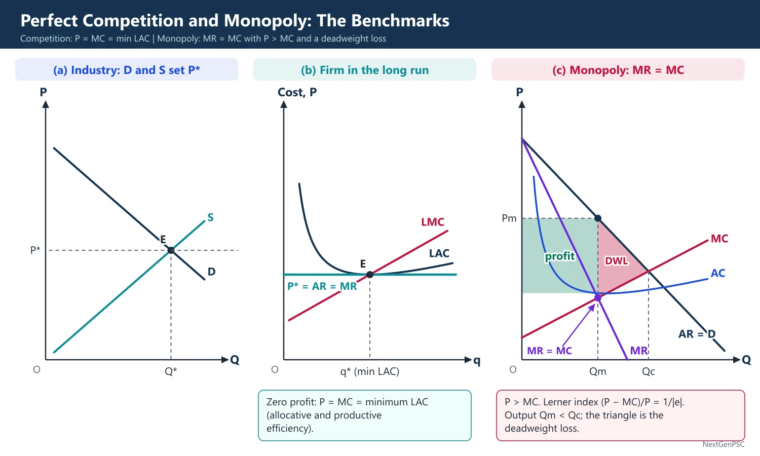
Perfect competition gives P = MC = minimum LAC in the long run: allocative and productive efficiency. A monopolist sets MR = MC with P > MC, measured by the Lerner index (P − MC)/P = 1/|e|, causing a deadweight loss. All other market forms are judged against these two benchmarks.
In simple words
Perfect competition is a market with so many small sellers of the same product that nobody can change the price, like vegetable sellers in a big mandi.
A monopoly is a single seller with no close substitute, like a railway in a region; it can raise the price by selling less.
Comparing the two shows how market power raises prices and wastes welfare.
UPSC uses them as benchmarks, asking you to compare outcomes and explain price discrimination and the Lerner index.
1. Why benchmarks
Market structure: classification of markets by the number of sellers, the nature of the product, entry conditions and control over price.
Benchmarks: perfect competition and pure monopoly are the two ends of the spectrum; monopolistic competition, duopoly and oligopoly lie in between and are judged against them.
Efficiency yardsticks: allocative efficiency (P = MC), productive efficiency (output at minimum average cost) and dynamic efficiency (innovation over time).
2. Perfect competition
Assumptions: many buyers and sellers, homogeneous product, free entry and exit, perfect knowledge, perfect factor mobility, no transport costs; each firm is a price taker.
Demand facing the firm: horizontal at the market price, so P = AR = MR.
Profit maximisation: MR = MC with MC rising (second-order condition: MC cuts MR from below).
Short run: a firm may earn supernormal profit or make a loss; it keeps producing as long as P ≥ minimum AVC (the shutdown point); its short-run supply curve is the MC curve above minimum AVC.
Long run: entry and exit drive economic profit to zero: P = MR = SMC = LMC = SAC = minimum LAC.
Industry supply: constant, increasing and decreasing cost industries give horizontal, rising and falling long-run supply curves (Marshall's external economies and diseconomies).
Welfare: P = MC gives allocative efficiency, output at minimum LAC gives productive efficiency, and the sum of consumer and producer surplus is maximised.
3. Monopoly
Definition: a single seller of a product with no close substitutes, protected by barriers to entry.
Sources of monopoly power: legal (patents, licences, statutory monopoly such as Indian Railways), control of essential inputs, economies of scale (natural monopoly) and network effects.
Revenue: demand slopes down and MR = P(1 − 1/|e|), so MR is positive only where demand is elastic; a profit-maximising monopolist never produces on the inelastic part of demand.
Equilibrium: MR = MC with MC cutting MR from below; price is read off the demand curve and exceeds MC.
Lerner index: L = (P − MC)/P = 1/|e| (Abba Lerner, 1934), a measure of monopoly power ranging from 0 under competition towards 1.
No supply curve: the same price can go with different quantities depending on the elasticity of demand, so there is no unique price-quantity supply relation.
Long run: profits can persist because entry is blocked; output is usually below the minimum-LAC output.
Multi-plant monopoly: output is allocated so that MC₁ = MC₂ = MR.
4. Price discrimination
Definition: selling the same product at different prices to different buyers for reasons not related to cost; A.C. Pigou (The Economics of Welfare, 1920) distinguished three degrees.
First degree: each unit is sold at the buyer's maximum willingness to pay; all consumer surplus is captured and output equals the competitive output.
Second degree: prices vary with the quantity bought (block tariffs, e.g. electricity slabs).
Third degree: separate markets (e.g. students and adults, domestic and export); condition MR₁ = MR₂ = MC, so P₁(1 − 1/|e₁|) = P₂(1 − 1/|e₂|) and the price is higher in the market with less elastic demand.
Conditions: market power, markets that can be separated with no resale, and different elasticities.
Welfare: third-degree discrimination can raise welfare only if it raises total output (Joan Robinson, 1933; Schmalensee, 1981); it can make possible a service that would otherwise not be supplied (e.g. railway class fares, medicines priced lower in poor countries).
5. Welfare costs and debates
Deadweight loss: the triangle between demand and MC from the monopoly output to the competitive output; Arnold Harberger (1954) estimated it at about 0.1% of US national income, which provoked a long debate.
X-inefficiency: Harvey Leibenstein (1966) argued that firms protected from competition do not minimise costs.
Rent-seeking: Gordon Tullock (1967) and Richard Posner (1975) argued that resources spent to obtain and defend monopoly add to its social cost; Anne Krueger (1974) applied the idea to import licences in India and Turkey.
Schumpeterian defence: monopoly profits finance research, and 'creative destruction' replaces old monopolies with new ones (Schumpeter, Capitalism, Socialism and Democracy, 1942).
Contestable markets: Baumol, Panzar and Willig (1982): if entry and exit are free and costless, even a single firm must price at average cost for fear of hit-and-run entry.
Natural monopoly regulation: marginal cost pricing (P = MC) causes losses when AC is falling; the options are average cost pricing, two-part tariffs, Ramsey pricing or public ownership.
6. Diagrams to draw
Perfect competition: two panels; on the left, industry D and S set the price P*; on the right, the firm faces a horizontal line P* = AR = MR with U-shaped AC and MC; equilibrium where MC = MR; in the long run AR is tangent to the minimum point of LAC.
Monopoly: a downward AR, MR below it with twice the slope (linear case), MC and AC; at Qm where MR = MC read Pm on AR; shade the profit rectangle (Pm − AC) × Qm; mark the competitive output Qc where AR = MC and shade the deadweight-loss triangle between Qm and Qc.
Third-degree discrimination: three panels: market 1 (less elastic), market 2 (more elastic), and combined MR with MC; equate combined MR to MC, then read MR₁ = MR₂ = MC and the two prices, higher in market 1.
7. Indian applications
Competition law: the Competition Act, 2002 replaced the MRTP Act, 1969; the Competition Commission of India (CCI) became fully functional in 2009; the Competition (Amendment) Act, 2023 added a deal-value threshold for merger review.
Abuse of dominance: the CCI imposed a penalty of ₹1,337.76 crore on Google in October 2022 for abuse of dominance in the Android ecosystem.
Natural monopolies: Indian Railways, power transmission and urban water supply are publicly owned or regulated; electricity regulatory commissions set cost-based tariffs.
Price control: essential medicines are capped under the Drugs (Prices Control) Order, 2013, administered by the National Pharmaceutical Pricing Authority.
8. Using it in the exam
10 marks: the relation MR = P(1 − 1/|e|), the Lerner index, and why a monopolist has no supply curve.
15 marks: monopoly equilibrium with a diagram, deadweight loss and comparison with perfect competition.
20 marks: add price discrimination with its condition, rent-seeking and X-inefficiency, contestability and CCI examples.
Keywords: price taker, P = MC, shutdown point, Lerner index, deadweight loss, price discrimination, natural monopoly, contestable market.
Formula to quote: Lerner index L = (P − MC)/P = 1/|e|.
| Basis | Perfect competition | Monopoly |
|---|---|---|
| Demand facing firm | Horizontal: P = AR = MR | Downward-sloping: MR below AR |
| Equilibrium | P = MC | MR = MC, P > MC |
| Long-run profit | Zero (normal profit) | Can be positive (entry blocked) |
| Output level | At minimum LAC | Usually below minimum LAC |
| Supply curve | MC above minimum AVC | None |
| Welfare | Surplus maximised | Deadweight loss; possible X-inefficiency and rent-seeking |
Mains points
- Derive MR = P(1 − 1/|e|) and use it to show why a monopolist operates only on the elastic part of demand.
- Use the Lerner index to measure market power and link it to elasticity; in oligopoly it becomes sᵢ/|e|.
- Draw the monopoly diagram with profit rectangle and deadweight-loss triangle side by side with the competitive outcome.
- For price discrimination, state the three degrees, the conditions and the rule MR₁ = MR₂ = MC, and discuss welfare through the output effect.
- Balance the static welfare loss with the Schumpeterian and contestable-markets arguments.
- Illustrate with Indian competition policy: CCI's Google order (2022), natural monopoly regulation and drug price control.
Did you know?
- Memory trick: a monopolist 'never sells where demand is inelastic', because there MR is negative and cutting output would raise both revenue and profit.
Monopolistic Competition (Chamberlin and Robinson)
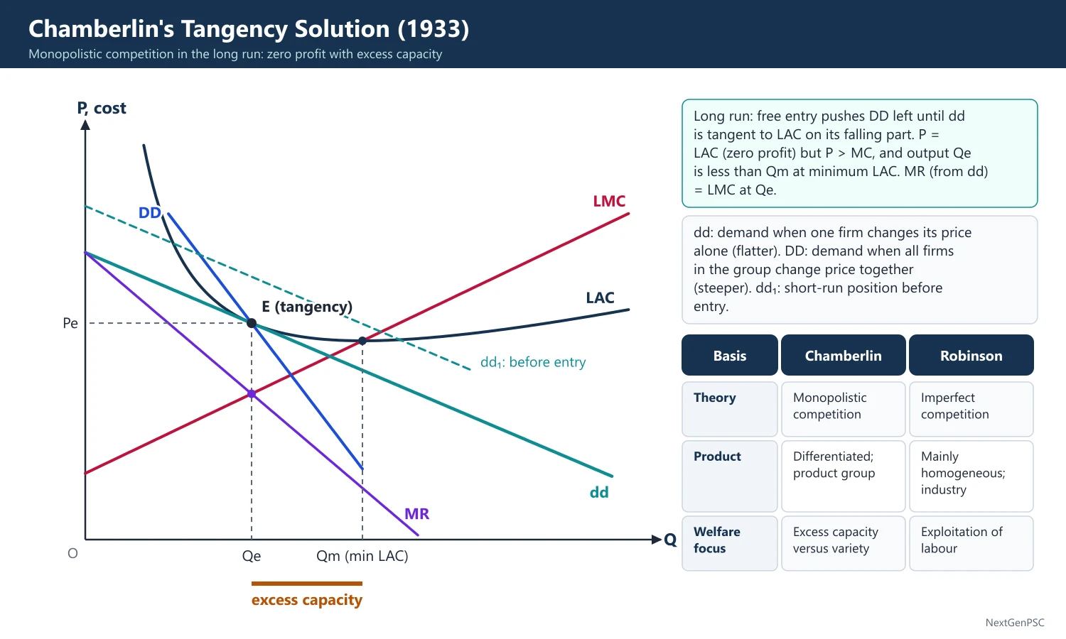
Chamberlin and Joan Robinson (both 1933) analysed markets between competition and monopoly. In Chamberlin's model many firms sell differentiated products with free entry; in the long run the firm's demand curve is tangent to LAC, giving zero profit, P > MC and excess capacity. Robinson stressed imperfect competition, price discrimination and monopsonistic exploitation of labour.
In simple words
Monopolistic competition is a market with many sellers whose products are similar but not identical, like restaurants or shampoo brands.
Each seller has a small monopoly over its own brand, but easy entry means profits disappear in the long run, just as a new café opens when one street café does well.
Firms end up a little smaller than the cheapest size: this is called excess capacity, the cost of variety.
UPSC asks you to draw the tangency diagram and compare Chamberlin with Robinson.
1. Concepts and definitions
Monopolistic competition: many firms selling differentiated products that are close but not perfect substitutes, with free entry; the term is Edward Chamberlin's, from The Theory of Monopolistic Competition (1933).
Imperfect competition: Joan Robinson's The Economics of Imperfect Competition (1933) analysed markets in which firms face downward-sloping demand, using marginal revenue as the key tool.
Product differentiation: real (quality, design, location) or perceived (brand, advertising); it gives each firm a small monopoly over its own brand.
Product group: Chamberlin's term for firms producing close substitutes, replacing the 'industry' of a homogeneous good.
Selling costs: costs incurred to shift the demand curve (advertising, salesmen, display), distinct from production costs; this was Chamberlin's original contribution.
2. Chamberlin's assumptions
Large group: many firms, each small enough to ignore rivals' reactions (symmetry assumption).
Uniformity ('heroic' assumption): all firms have identical cost and demand curves despite product differentiation.
Entry: free entry and exit in the long run.
Choice variables: each firm chooses price, product variety and selling outlay.
3. Short and long-run equilibrium
Two demand curves: dd is the firm's perceived demand when it alone changes price (more elastic); DD is the share-of-market demand when all firms in the group change price together (less elastic).
Short run: the firm sets MR (from dd) = MC and may earn supernormal profit if price exceeds AC.
Adjustment: each firm, believing in dd, cuts price to raise sales; all do so, so each firm actually moves down DD and dd slides down along DD.
Entry: supernormal profits attract new firms, shifting DD to the left as each firm's share falls.
Long-run equilibrium (tangency solution): dd is tangent to LAC at the point where DD cuts it; P = LAC (zero economic profit) and MR = LMC at that output.
Result: price exceeds marginal cost (P > MC) and output lies on the falling part of LAC.
4. Excess capacity
Definition: the difference between the output at minimum LAC (the 'ideal' output of perfect competition) and the actual tangency output.
Cause: the downward-sloping demand curve from product differentiation can be tangent to LAC only on its falling part.
Chamberlin's view: excess capacity is partly the price paid for variety, so it is not wholly waste; with free entry there are too many firms, each below optimum scale.
Kaldor (1935): argued that excess capacity means unexploited economies of scale, and that tangency is not assured because a new entrant takes customers mainly from its nearest neighbours, not from the whole group.
Non-price competition: where firms avoid price cuts and compete through advertising, excess capacity can be larger.
5. Selling costs and product variation
Selling costs: shift and steepen the demand curve; an average selling cost curve is added to average production cost; the firm advertises until the marginal revenue from extra advertising equals its marginal cost.
Dorfman-Steiner condition (1954): the optimal advertising-to-sales ratio equals the advertising elasticity of demand divided by the price elasticity of demand.
Product variation: firms choose quality and design as variables, each with its own cost and demand effects.
Debate on advertising: informative advertising lowers search costs and helps entry; persuasive advertising raises barriers and prices (Galbraith's 'dependence effect' in The Affluent Society, 1958).
6. Robinson's contribution and the differences
Tools: Robinson popularised the marginal revenue curve and the MR = MC rule for all market forms.
Price discrimination: she gave a detailed analysis of third-degree discrimination and its output effects.
Monopsony and exploitation: building on Pigou's definition (wage below the value of marginal product, VMP), she separated monopolistic exploitation (VMP − MRP, from product-market power) and monopsonistic exploitation (MRP − wage, from labour-market power).
Chamberlin versus Robinson: Chamberlin stressed product differentiation, selling costs and group equilibrium; Robinson stressed imperfection in an industry with a homogeneous product, price discrimination and factor exploitation; Chamberlin insisted that the two theories were different.
7. Criticisms
Group concept: Robert Triffin (1940) argued that with differentiated products every firm competes with every other to some degree, so the 'group' cannot be defined.
Heroic assumptions: identical cost and demand curves contradict product differentiation.
Stigler (1949): argued that monopolistic competition yields few predictions not available from perfect competition or monopoly.
Long-run pricing: Harrod (1952) and P.W.S. Andrews argued that firms set prices with an eye on potential entry, which reduces excess capacity.
Empirical relevance: retail, restaurants, consumer goods and services fit the model well, even if its precise tangency result is hard to test.
8. Diagrams to draw
Long-run tangency: axes Q and P; draw U-shaped LAC and LMC, a flat dd tangent to LAC at E on its falling part, a steeper DD passing through E, and MR (from dd) cutting LMC at the tangency output Qe; mark the minimum-LAC output Qm to the right; the distance from Qe to Qm is excess capacity.
Adjustment path: show dd1 above, sliding down DD as all firms cut prices, and DD shifting left with entry until tangency.
Selling costs: add an average selling cost curve on top of average production cost to get average total cost; show the demand shift from advertising and the new equilibrium.
9. India and the exam
Indian examples: consumer brands (soaps, tea, biscuits), restaurants, apparel, salons and coaching centres, with heavy brand advertising by consumer goods firms.
10 marks: features, tangency solution and excess capacity in one diagram.
15 marks: dd and DD curves, adjustment, long-run equilibrium, excess capacity and selling costs.
20 marks: compare Chamberlin and Robinson, criticisms (Triffin, Kaldor, Stigler), welfare (variety versus excess capacity) and an Indian example.
Keywords: product differentiation, product group, dd and DD, tangency solution, excess capacity, selling costs, heroic assumption.
Definition: excess capacity is the gap between the output at minimum long-run average cost and the actual long-run equilibrium output.
| Basis | Chamberlin (1933) | Joan Robinson (1933) |
|---|---|---|
| Title of theory | Monopolistic competition | Imperfect competition |
| Product | Differentiated; product group | Mainly homogeneous; industry |
| Key ideas | dd and DD curves, tangency, selling costs, product variation | MR curve, price discrimination, monopsony |
| Welfare focus | Excess capacity versus variety | Exploitation of labour (monopolistic and monopsonistic) |
| Main critics | Triffin, Kaldor, Stigler | Chamberlin, who stressed differences |
Mains points
- Draw the long-run tangency diagram with both dd and DD; many answers show only one demand curve and lose marks.
- Define excess capacity precisely and discuss whether it is waste or the price of variety.
- Explain selling costs as a distinctive feature, with the Dorfman-Steiner condition for a high-scoring answer.
- Compare Chamberlin and Robinson in a table, including Robinson's monopsonistic exploitation.
- Criticise with Triffin's group problem, the heroic assumptions and Kaldor's excess-capacity argument.
- Give Indian examples from consumer goods, restaurants or coaching, and note the role of brand advertising.
Did you know?
- Chamberlin and Robinson published their books in the same year, 1933, independently, and Chamberlin spent years insisting that his 'monopolistic competition' was not the same as her 'imperfect competition'.
Duopoly Models: Cournot, Bertrand, Stackelberg and Edgeworth
In Cournot (1838) two firms choose quantities, each taking the rival's output as given; with linear demand each produces one-third of the competitive output. In Bertrand (1883) firms choose prices and undercut to P = MC. Stackelberg (1934) adds a leader with a first-mover advantage, and Edgeworth (1897) shows that capacity limits cause prices to oscillate.
In simple words
A duopoly is a market with only two sellers, so each must guess how the other will react.
It is like two tea stalls at a railway platform: if one cuts prices, the other may match; if one stocks more, the other may stock less.
Different guesses give different results: Cournot (choose quantity), Bertrand (choose price), Stackelberg (one moves first) and Edgeworth (limited capacity).
UPSC asks you to derive the equilibria, draw reaction curves and compare the models.
1. Concepts and definitions
Duopoly: a market with two sellers; each firm's profit depends on the other's decision, so the outcome depends on what each assumes about the rival's reaction.
Conjectural variation: the change a firm expects in the rival's output (or price) when it changes its own; zero conjectural variation is the Cournot-Nash assumption.
Reaction function: the best output (or price) of one firm for each output (or price) of the rival.
Nash equilibrium: a pair of strategies in which each is the best response to the other (John Nash, 1950–51); the Cournot equilibrium is a Nash equilibrium in quantities.
2. Cournot model (1838)
Source: Augustin Cournot, Recherches sur les principes mathématiques de la théorie des richesses (1838), with the example of two owners of mineral springs producing at zero cost.
Assumptions: homogeneous product; two firms choose quantities simultaneously; each assumes the rival's output stays fixed; linear demand P = a − b(q₁ + q₂); constant marginal cost c.
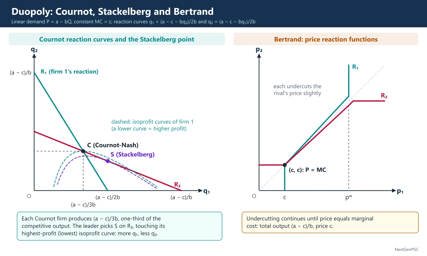
Reaction functions: firm 1 maximises (a − bq₁ − bq₂ − c)q₁, giving q₁ = (a − c − bq₂)/(2b); similarly q₂ = (a − c − bq₁)/(2b).
Equilibrium: q₁ = q₂ = (a − c)/(3b); total output 2(a − c)/(3b); price P = (a + 2c)/3.
Comparison: monopoly output is (a − c)/(2b) and competitive output (a − c)/b, so Cournot duopoly produces two-thirds of the competitive output; with n firms total output is n/(n + 1) of the competitive output, approaching competition as n grows.
Mark-up rule: (P − MC)/P = sᵢ/|e|, where sᵢ is the firm's market share; the industry average equals HHI/|e|, linking concentration to market power.
Stability: with linear demand, step-by-step adjustment along the reaction curves converges to their intersection.
Criticism: firms never learn that rivals do react, and the model is static; still, it remains the workhorse model of quantity competition.
3. Bertrand model (1883)
Source: Joseph Bertrand's 1883 review of Cournot argued that firms choose prices, not quantities.
Assumptions: homogeneous product, identical constant MC = c, no capacity limits; consumers buy from the cheaper firm and split equally at equal prices.
Result: each firm undercuts the other until P₁ = P₂ = c, and profits are zero.
Bertrand paradox: two firms are enough to give the competitive outcome.
Resolutions: capacity constraints (Edgeworth; Kreps and Scheinkman, 1983, showed that capacity choice followed by price competition gives the Cournot outcome), product differentiation (prices above MC) and repeated interaction (tacit collusion).
4. Edgeworth model (1897)
Source: F.Y. Edgeworth (1897) introduced capacity limits into price competition.
Mechanism: neither firm can supply the whole market; if the rival charges a low price and sells to capacity, the other can raise its price on the residual demand; the rival then raises its price too, and then each undercuts again.
Result: there is no stable equilibrium; the price oscillates between an upper and a lower limit (the Edgeworth cycle).
Relevance: retail petrol price cycles observed in some countries are cited as Edgeworth cycles.
5. Stackelberg model (1934)
Source: Heinrich von Stackelberg, Marktform und Gleichgewicht (1934).
Assumptions: one firm (the leader) moves first, knowing the follower's reaction function; the follower behaves as in Cournot.
Solution: the leader maximises (a − bq_L − bR(q_L) − c)q_L, where R is the follower's reaction function; this gives q_L = (a − c)/(2b), q_F = (a − c)/(4b), total output 3(a − c)/(4b) and P = (a + 3c)/4.
First-mover advantage: the leader produces and earns more than in Cournot and the follower less; total output is higher and price lower than in Cournot.
Stackelberg disequilibrium: if both firms try to lead they over-produce and a price war follows; if both choose to follow, the Cournot outcome results.
Chamberlin's solution (1929, 1933): recognising mutual dependence, duopolists would each produce half the monopoly output and share the monopoly profit, even without explicit agreement.
6. Diagrams to draw
Cournot: axes q₁ (horizontal) and q₂ (vertical); firm 1's reaction curve runs from (a − c)/(2b) on the q₁ axis to (a − c)/b on the q₂ axis, firm 2's is symmetric; mark the intersection C as the Cournot-Nash equilibrium; draw firm 1's isoprofit curves as inverted U-shapes peaking on its reaction curve, lower curves meaning higher profit.
Stackelberg: on the same diagram find the point S on firm 2's reaction curve where firm 1's highest-profit isoprofit curve is tangent; S lies to the right of C (more q₁, less q₂).
Bertrand: axes p₁ and p₂; each reaction function lies just below the rival's price, down to c; the only intersection is at (c, c).
Edgeworth: a demand diagram split into two halves with capacity limits; show the price jumping between the upper and lower limits.
7. Applications
Indian telecom: after 2016, Reliance Jio's low prices forced exits and mergers, leaving two strong private firms and a weak third; both capacity (quantity) and price competition matter.
Digital payments: PhonePe and Google Pay handle the large majority of UPI transactions; the NPCI has proposed a market-share cap to limit concentration, but its implementation has been deferred.
World: Boeing and Airbus in large commercial aircraft (a classic duopoly and a case for strategic trade policy); Coca-Cola and PepsiCo in soft drinks.
8. Using it in the exam
10 marks: Cournot assumptions, reaction functions and the two-thirds result.
15 marks: Cournot versus Bertrand, with the paradox and its resolutions.
20 marks: Cournot, Bertrand, Stackelberg and Edgeworth with reaction-curve diagrams, a comparison table and criticism.
Keywords: conjectural variation, reaction function, Nash equilibrium, isoprofit curve, Bertrand paradox, first-mover advantage, capacity constraint.
Quotable result: in Cournot duopoly with linear demand and constant cost, each firm produces one-third of the competitive output and the industry two-thirds.
| Model | Choice variable and timing | Conjecture | Total output | Price |
|---|---|---|---|---|
| Cournot (1838) | Quantity, simultaneous | Rival's output fixed | 2(a − c)/(3b) | (a + 2c)/3 |
| Bertrand (1883) | Price, simultaneous | Rival's price fixed | (a − c)/b | c |
| Stackelberg (1934) | Quantity, leader first | Leader knows follower's reaction | 3(a − c)/(4b) | (a + 3c)/4 |
| Edgeworth (1897) | Price with capacity limits | Rival's price fixed | Indeterminate | Oscillates between limits |
| Collusion / monopoly | Joint quantity | Joint profit maximisation | (a − c)/(2b) | (a + c)/2 |
Mains points
- Derive the Cournot reaction functions and equilibrium algebraically with linear demand; numerical versions are common.
- Draw reaction curves with isoprofit curves; show the Cournot point C and the Stackelberg point S on one diagram.
- Explain the Bertrand paradox and give at least two resolutions (capacity limits, product differentiation).
- Rank outputs: monopoly less than Cournot less than Stackelberg less than Bertrand (competitive); prices in the reverse order.
- Mention that Cournot is a Nash equilibrium and that the Kreps-Scheinkman result reconciles Cournot and Bertrand.
- Add an application: Indian telecom consolidation, UPI concentration, or Boeing-Airbus.
Did you know?
- Memory trick for outputs with linear demand: monopoly 1/2, Cournot 2/3, Stackelberg 3/4, Bertrand 1 (as fractions of the competitive output).
Oligopoly: Kinked Demand, Collusion, Price Leadership and Game Theory
Oligopoly is a market of a few interdependent sellers. The kinked demand curve (Sweezy; Hall and Hitch, 1939) explains price rigidity through a gap in MR. Cartels maximise joint profit but are unstable because members cheat; price leadership is a looser form of coordination. Game theory (Nash equilibrium, prisoner's dilemma, repeated games) gives the modern framework.
In simple words
Oligopoly is a market with a few big sellers, like telecom companies or cement makers, where each watches the others closely.
It resembles a game of chess: every move depends on what you expect the rival to do next.
Firms may keep prices steady, form secret agreements (cartels), follow a leader, or fight price wars.
UPSC asks you to draw the kinked demand curve, explain cartel instability and use the prisoner's dilemma.
1. Concepts and definitions
Oligopoly: a few large sellers, homogeneous or differentiated products, high barriers to entry and mutual interdependence in decisions; there is no single theory of oligopoly, because outcomes depend on assumed rival behaviour.
Non-collusive models: Cournot, Bertrand, Stackelberg (previous topic) and the kinked demand curve.
Collusive models: cartels and price leadership.
Strategic models: game theory (John von Neumann and Oskar Morgenstern, Theory of Games and Economic Behavior, 1944; John Nash, 1950–51).
Measuring concentration: the concentration ratio (share of the top 4 or 8 firms) and the Herfindahl-Hirschman Index (HHI = sum of squared market shares); a higher HHI means a more concentrated market, and competition authorities use HHI thresholds in merger review.
2. Kinked demand curve
Authors: Paul Sweezy (Journal of Political Economy, 1939) and, independently, R.L. Hall and C.J. Hitch (Oxford Economic Papers, 1939).
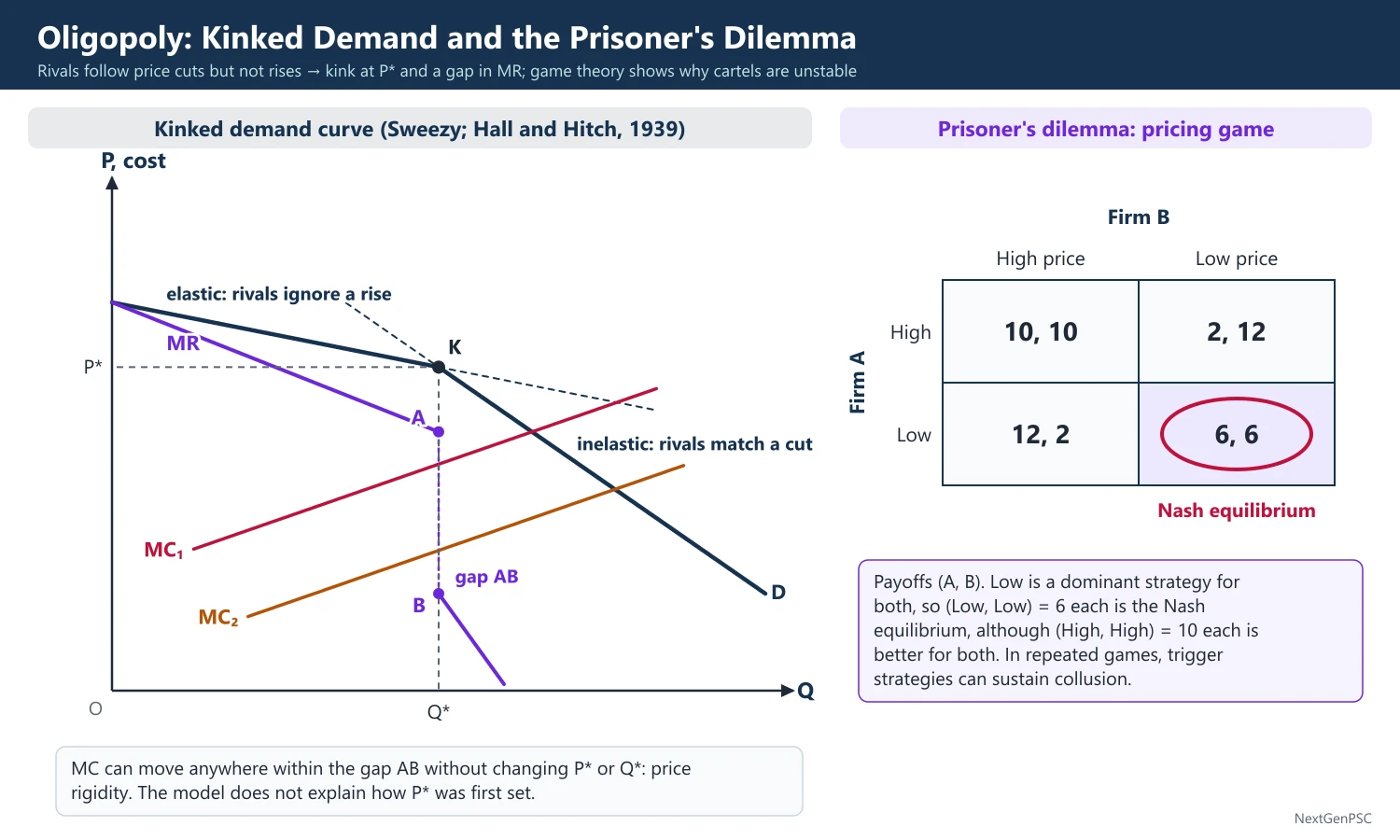
Assumption: rivals match a price cut (to protect market share) but do not follow a price rise (to gain customers).
Demand: elastic above the current price and inelastic below it, so the demand curve has a kink at the prevailing price.
Marginal revenue: discontinuous, with a vertical gap at the kink output.
Price rigidity: MC can shift up or down within the gap without changing the profit-maximising price and output; demand shifts that keep the kink at the same price also leave price unchanged.
Full-cost pricing: Hall and Hitch also found that firms set prices at average cost plus a conventional margin rather than by MR = MC.
Criticism: the model explains why price stays at the kink, not how that price was first set; George Stigler (1947) found little evidence of greater price rigidity in oligopolies; in inflation firms readily follow price rises, so the kink can reverse.
3. Collusion and cartels
Cartel: a formal agreement among firms to fix prices, output or market shares.
Joint profit maximisation: the cartel acts like a multi-plant monopolist: industry MR = MC₁ = MC₂, with output quotas set so that members' marginal costs are equal.
Market-sharing cartel: quotas or territories (often by historical share) instead of a cost-efficient allocation.
Instability: each member gains by secretly producing more at the cartel price (for it, the price exceeds MC); cheating, entry and demand shocks break cartels.
Conditions for success: few members, similar costs, homogeneous product, inelastic demand, barriers to entry and the ability to detect and punish cheating.
OPEC: founded in 1960 in Baghdad and headquartered in Vienna; with Russia and other producers it has worked as OPEC+ since 2016, setting production targets; oil prices still swing widely because of cheating and non-member supply such as US shale.
India: the CCI penalised cement companies for cartelisation (order of 2012, re-issued in 2016) and tyre makers (order of 2018, made public in 2022).
4. Price leadership
Dominant-firm leadership: a large firm sets the price; small fringe firms act as price takers and sell where P = their MC; the dominant firm faces the residual demand (market demand minus fringe supply) and sets its MR from residual demand equal to its MC.
Low-cost firm leadership: the firm with the lowest cost sets a price that others accept because they cannot undercut it profitably.
Barometric leadership: a firm that reads market conditions best announces price changes that others follow, without being dominant.
Indian example: telecom operators raised tariffs within days of each other in December 2019 and in July 2024; such parallel pricing is consistent with price leadership, though parallel pricing alone does not prove collusion under competition law.
5. Game theory
Elements: players, strategies, payoffs, information and timing.
Dominant strategy: a strategy that is best whatever the rival does.
Nash equilibrium: no player can gain by changing strategy on its own.
Prisoner's dilemma: named by Albert Tucker (1950) from a game devised by Merrill Flood and Melvin Dresher; two firms choose a high or low price: (High, High) gives 10 each, (Low, Low) 6 each, and Low against High gives 12 to the low-price firm and 2 to the other; Low is dominant for both, so (Low, Low) is the Nash equilibrium although (High, High) is better for both.
Repeated games: if the game is repeated indefinitely, trigger strategies (cooperate until the rival cheats, then punish) can sustain collusion; in a symmetric Bertrand game with n firms collusion is sustainable if the discount factor δ ≥ 1 − 1/n (δ ≥ 1/2 for two firms); Robert Axelrod (1984) showed the strength of tit-for-tat.
Sequential games and credibility: Reinhard Selten's subgame perfection (1965) rules out non-credible threats; an incumbent's threat of a price war is credible only if fighting is profitable after entry.
Entry deterrence: limit pricing (Joe Bain, 1956; Paolo Sylos-Labini, 1957): incumbents keep price low enough to make entry unprofitable; excess capacity can be a credible commitment (Spence, 1977; Dixit, 1980).
6. Diagrams to draw
Kinked demand: axes Q and P; draw a flat demand segment above the price P* and a steep segment below it, meeting at K; draw the two MR segments with a vertical gap AB below K; draw MC₁ and MC₂ both passing through the gap; price stays at P* and output at Q*.
Dominant firm: draw market demand D and fringe supply Sf; residual demand Dr = D − Sf; draw MRr and the dominant firm's MC; at their intersection read its output Qd and the price P from Dr; the fringe supplies along Sf at P.
Cartel: two panels for firms 1 and 2 with MC₁ and MC₂, and a third panel with industry D, MR and ΣMC; read the cartel price where MR = ΣMC and allocate quotas where MC₁ = MC₂ = MR.
Payoff matrix: draw a 2 × 2 table with the four payoff pairs and circle the Nash equilibrium.
7. Debates and India
Other objectives: Baumol's sales-revenue maximisation (1959) and other managerial theories argue that oligopolists may not maximise profit.
Contestability: if entry is easy, even a concentrated market may behave competitively (Baumol, Panzar and Willig, 1982).
Indian relevance: concentration in telecom, aviation, cement, tyres and digital platforms keeps oligopoly questions live for the CCI; the Competition (Amendment) Act, 2023 introduced settlement and commitment procedures.
8. Using it in the exam
10 marks: the kinked demand curve with its MR gap and price rigidity, plus one criticism.
15 marks: cartel joint profit maximisation, instability and the OPEC example.
20 marks: compare kinked demand, cartel, price leadership and game theory, with the prisoner's dilemma matrix and an Indian example.
Keywords: mutual interdependence, kink, MR gap, price rigidity, joint profit maximisation, cheating, dominant firm, Nash equilibrium, prisoner's dilemma, trigger strategy.
Quotable point: the kinked demand curve explains price rigidity but not the level of the price (Stigler, 1947).
| Model | Key assumption | Result | Main weakness |
|---|---|---|---|
| Kinked demand (Sweezy; Hall and Hitch, 1939) | Rivals follow cuts, not rises | Price rigidity through MR gap | Does not explain the initial price |
| Cartel | Explicit agreement on output or price | Joint profit maximisation (monopoly outcome) | Incentive to cheat; illegal under competition law |
| Dominant-firm leadership | Fringe firms are price takers | Leader sets price on residual demand | Fringe growth erodes leadership |
| Game theory (Nash, 1950–51) | Rational players choose best responses | Nash equilibrium; collusion possible in repeated games | Multiple equilibria; outcome sensitive to assumptions |
Mains points
- Draw the kinked demand curve with the MR gap and show MC shifting within the gap; give the correct authors (Sweezy; Hall and Hitch, 1939).
- State the cartel condition MR = MC₁ = MC₂ and explain why each member has an incentive to cheat.
- Explain dominant-firm price leadership with the residual-demand diagram.
- Use a numerical prisoner's dilemma matrix to show why oligopolists may end up in a price war, and repeated games to show how collusion can survive.
- Link to India: CCI cartel cases (cement, tyres), parallel telecom tariff hikes, and OPEC's effect on India's import bill.
- Avoid saying the kinked demand curve explains price determination; it explains only rigidity.
Did you know?
- John Nash's equilibrium idea came from a doctoral thesis of under 30 pages (Princeton, 1950); he shared the 1994 Nobel Prize with Harsanyi and Selten.
UPSC Previous Year Questions: Market Structures
UPSC asked 30 question parts worth 425 marks from market structures between 2014 and 2026, all in Paper I. Duopoly models (9 parts, several numerical) and oligopoly with game theory (9 parts) dominate, followed by monopolistic competition (7) and the perfect competition and monopoly benchmarks (5). Every question below has a model answer written to the UPSC word limit, with full working for the numericals.
In simple words
Attempt each question yourself first, using the Approach line as a hint, and for numericals write every step before checking.
Then compare with the model answer: check the equilibrium condition, the reaction functions, the diagram and the final numbers.
Mark the questions you got wrong and redo them after a week without looking at the solution.
1. Perfect Competition and Monopoly: The Benchmarks
Example 1 (UPSC 2023, 10 marks): Examine the role of price elasticity of demand in determining the price set by a discriminating monopolist.
Paper and question: Paper I, Q1(a)
Approach: State the profit-maximising condition for third-degree discrimination, derive the inverse-elasticity pricing rule, and show that the less elastic market gets the higher price.
Price discrimination (Pigou, The Economics of Welfare, 1920) means selling the same product at different prices to different buyers for reasons not related to cost. In third-degree discrimination the monopolist divides buyers into markets that cannot resell to each other.
Condition: profit is maximised where MR₁ = MR₂ = MC: if MR were higher in one market, shifting a unit there would raise revenue.
Role of elasticity: since MR = P(1 − 1/e), the condition gives P₁(1 − 1/e₁) = P₂(1 − 1/e₂). Hence P₁/P₂ = (1 − 1/e₂)/(1 − 1/e₁), so the market with the lower elasticity gets the higher price. If elasticities are equal, discrimination is not profitable. Equivalently, the mark-up rule (P − MC)/P = 1/e holds in each market.
Diagram: three panels: market 1 with steep (inelastic) D₁ and MR₁, market 2 with flatter D₂ and MR₂, and the aggregate ΣMR cutting MC at total output; a horizontal line from that point gives q₁ and q₂ where MR₁ and MR₂ equal MC, with P₁ above P₂.
Examples: Indian Railways' class-wise fares, student discounts and airline fares by booking time; telecom plans for different users. Elasticity is thus the key that decides both whether to discriminate and how much.
Example 2 (UPSC 2023, 15 marks): "Perfect competition is incompatible with increasing returns to scale." Examine the statement.
Paper and question: Paper I, Q2(b)
Approach: Explain why increasing returns make marginal cost lie below average cost, so that price = MC gives losses and firms grow until competition breaks down; add Sraffa's critique and the ways out (external economies, Marshall).
Perfect competition requires many price-taking firms, each producing where P = MC with MC rising. Increasing returns to scale mean that a proportionate rise in all inputs raises output more than proportionately, so long-run average cost (LAC) falls as output grows.
Incompatibility: (i) with falling LAC, LMC lies below LAC, so a price equal to MC is below average cost and every firm makes a loss; the P = MC equilibrium cannot be sustained. (ii) If price exceeds the cost of a larger firm, each firm gains by expanding, since unit cost keeps falling; the second-order condition fails. (iii) Firms grow until they are large relative to the market and stop being price takers: competition gives way to oligopoly or natural monopoly.
Sraffa's critique ('The Laws of Returns under Competitive Conditions', Economic Journal, 1926) pressed exactly this point: internal economies of scale are inconsistent with competitive equilibrium, so firms are limited by demand, not cost, which pointed towards imperfect competition theory (Joan Robinson, 1933; Chamberlin, 1933).
Reconciliation: Marshall's external economies lower the industry's supply curve while each firm still faces rising costs, so decreasing-cost industries can be competitive.
Diagram: output on the horizontal and cost on the vertical axis; a falling LAC with LMC below it; a horizontal price line P = LMC at q₀ lies below LAC, showing a loss per unit equal to the gap.
Examples: power transmission, railways and telecom networks are natural monopolies regulated by bodies such as CERC and TRAI. The statement holds for internal, not external, economies of scale.
Example 3 (UPSC 2019, 10 marks): What determines the degree of price discrimination under monopoly market?
Paper and question: Paper I, Q1(b)
Approach: Define the degrees of discrimination (Pigou), then list the factors that decide how far a monopolist can discriminate: elasticity differences, separability, information and resale costs.
Pigou (1920) classified price discrimination into three degrees: first degree (each unit sold at the buyer's maximum willingness to pay, capturing all consumer surplus), second degree (prices vary with the quantity bought, e.g. block tariffs) and third degree (different prices in separated markets).
Determinants of the degree: (i) information: first degree needs each buyer's reservation price, rarely known, so most firms use second or third degree; (ii) separation of markets: resale must be impossible or costly, as with services or distant markets; (iii) elasticity differences: since P₁/P₂ = (1 − 1/e₂)/(1 − 1/e₁), wider differences allow wider price gaps; (iv) monopoly power: close substitutes or entry limit high prices; (v) cost of segmentation must be below the extra revenue; (vi) legal and social limits such as competition law.
Diagram: a downward demand curve with MC; under perfect discrimination output extends to where D cuts MC and the whole area under D above MC becomes profit; under simple monopoly output is where MR = MC.
Thus the degree depends on how well the seller can identify and separate buyers with different elasticities; digital platforms using data on users are moving closer to first-degree discrimination.
Example 4 (UPSC 2018, 10 marks): Explain some of the measures for assessing the monopoly power of a firm.
Paper and question: Paper I, Q1(b)
Approach: Define monopoly power and explain three or four measures (Lerner index, Bain's profit measure, concentration ratios and HHI, cross elasticity) with their formulas and limits.
Monopoly power is a firm's ability to raise price above marginal cost without losing all its sales. It is measured in several ways.
1. Lerner index (Abba Lerner, 1934): L = (P − MC)/P, between 0 (perfect competition) and 1; at the profit maximum L = 1/e. Its limitation is that MC is hard to observe.
2. Bain's profit measure (Joe Bain): persistent excess (supernormal) profit over the normal return on capital signals monopoly power, though accounting profits may differ from economic profits.
3. Concentration measures: the four-firm concentration ratio and the Herfindahl-Hirschman Index HHI = Σsᵢ² (up to 10,000 with shares in per cent); higher values mean less competition.
4. Cross elasticity of demand (Triffin): a low cross elasticity with rivals' prices means few close substitutes and greater independence of the firm.
The Competition Commission of India uses market shares, HHI and entry barriers together, since no single measure suffices.
Example 5 (UPSC 2015, 10 marks): Under perfect competition, in the short run, find out graphically, without using average cost curve, the conditions in equilibrium for the existence of (i) normal profit, (ii) supernormal profit and (iii) loss.
Paper and question: Paper I, Q1(b)
Approach: Use the price line together with the MC and AVC curves and the total revenue and total cost approach (no AC curve): compare price with AVC and total revenue with total cost at the MR = MC output.
A competitive firm takes price as given (P = MR) and produces where P = MC with MC rising. Without the AC curve, profit is read from the total revenue (TR) and total cost (TC) curves: TR is a ray from the origin with slope P.
Equilibrium: where the slope of TR (price) equals the slope of TC (MC), so TR − TC is greatest.
(i) Normal profit: the TR line is just tangent to the TC curve, so TR = TC at the best output; economic profit is zero (normal profit is included in costs).
(ii) Supernormal profit: TR lies above TC over a range; at the output where their slopes are equal, TR exceeds TC by the maximum gap.
(iii) Loss: TR lies below TC everywhere; the firm produces where the gap is smallest if TR covers total variable cost, since the loss is then below the fixed cost; otherwise it shuts down.
Diagram: output on the horizontal and rupees on the vertical axis; an S-shaped TC starting at TFC; three TR rays of rising slope: one tangent to TC (normal profit), one cutting it (profit gap marked), one below it (loss gap marked), each at the output where the TR slope equals the TC slope.
2. Monopolistic Competition (Chamberlin and Robinson)
Example 6 (UPSC 2024, 10 marks): Differentiate between perceived demand curve and proportional demand curve in a monopolistic competitive market. Explain why the proportional demand curve is steeper than the perceived demand curve.
Paper and question: Paper I, Q1(a)
Approach: Define Chamberlin's dd (perceived, ceteris paribus) and DD (proportional, share-of-market) curves and explain why DD is steeper.
In The Theory of Monopolistic Competition (1933), Edward Chamberlin gave each firm in a group of sellers of differentiated products two demand curves.
Perceived demand curve (dd): the demand the firm expects if it alone changes its price while rivals keep theirs unchanged. A price cut attracts customers from rivals as well as new buyers, so dd is relatively flat (elastic).
Proportional demand curve (DD): the demand the firm actually faces when all firms in the group change prices together. Each firm keeps a constant share (1/n) of the market demand, so DD is the firm's share of the market demand curve.
Why DD is steeper: when all firms cut price together, no firm gains customers from rivals; each gains only its share of the extra market demand. The quantity response to a given price change is therefore smaller along DD than along dd, so DD is less elastic and steeper.
Diagram: price on the vertical and quantity on the horizontal axis; a flat dd and a steeper DD crossing at the current price; a price cut along dd promises a large rise in sales, but because rivals follow, actual sales move along DD and dd slides down DD.
This gap explains why each firm keeps cutting price expecting gains, until the group reaches the tangency equilibrium.
Example 7 (UPSC 2024, 15 marks): Describe the short-run and long-run equilibrium of a firm under monopolistic competition.
Paper and question: Paper I, Q2(c)
Approach: Describe short-run equilibrium (MR = MC with profit or loss) and long-run equilibrium with free entry (tangency of AR with LAC), using Chamberlin's diagrams, and note excess capacity.
Monopolistic competition (Chamberlin, 1933) has many sellers of differentiated products, free entry and exit, and some control over price; each firm faces a downward-sloping but elastic demand curve.
Short run: the number of firms is fixed. Each firm produces where MR = MC (MC cutting MR from below) and charges the price read from its demand curve. If price exceeds short-run average cost it earns supernormal profit; if price is below average cost but above AVC it makes a loss yet continues production.
Diagram: short run: AR and MR falling, U-shaped SAC and SMC; MR = MC at Q₁, price P₁ on AR above SAC, the profit rectangle shaded. Long run: AR tangent to LAC at E on its falling portion, with MR = LMC at the same output Qₑ, which lies to the left of the LAC minimum Qₘ.
Long run: supernormal profits attract new firms with close substitutes; each firm's demand curve shifts left (and becomes more elastic) until it is tangent to the LAC curve. At the tangency, P = LAC, so only normal profit is earned, and MR = LMC at the same output. Losses work in reverse as firms exit. In Chamberlin's group analysis, dd becomes tangent to LAC at the point where it cuts DD.
Features: since the demand curve slopes down, the tangency lies on the falling part of LAC: output is below the minimum-cost output (excess capacity) and P exceeds MC, so there is allocative inefficiency.
Long-run equilibrium thus combines monopoly power (P greater than MC) with zero economic profit, as seen in restaurants, salons and apparel brands.
Example 8 (UPSC 2022, 10 marks): Explain briefly Chamberlin's concept of excess capacity in monopolistic competition.
Paper and question: Paper I, Q1(a)
Approach: Define excess capacity as the gap between the tangency output and the minimum-LAC output, show it with the tangency diagram, and note Chamberlin's distinction from 'ideal output' and the variety argument.
Excess capacity is the difference between the output at which long-run average cost is minimum (the optimum or competitive output) and the output a firm actually produces in long-run equilibrium under monopolistic competition.
Reason: with free entry, each firm's downward-sloping demand curve becomes tangent to its LAC curve. A downward-sloping line can touch a U-shaped curve only on its falling part, so equilibrium output Qₑ is less than the minimum-cost output Qₘ, and price (= LAC) exceeds minimum LAC. Too many firms each operate plants below their efficient scale.
Diagram: LAC U-shaped; a downward AR tangent to LAC at E (output Qₑ, price Pₑ); the minimum of LAC at M (output Qₘ); the distance QₑQₘ is excess capacity.
Chamberlin's view: excess capacity arises mainly under price competition with free entry; when firms avoid price competition and compete through selling costs and product variation, it can be larger still. Chamberlin argued that the comparison with the competitive 'ideal' is misleading, because differentiation gives consumers variety, which has value; excess capacity may be the price of choice.
Examples include many under-used shops and restaurants in a locality.
Example 9 (UPSC 2019, 20 marks): Reflect on the inefficiency and socially undesirable aspects of monopolistic competition market situation vis-à-vis the perfect competition, both in the short and in the long run.
Paper and question: Paper I, Q3(c)
Approach: Compare monopolistic competition with perfect competition in the short and long run on price, output, efficiency (allocative, productive), selling costs and welfare, with the tangency diagram, then give the counter-arguments.
Under perfect competition long-run equilibrium satisfies P = MC = minimum LAC: output is produced at the lowest cost (productive efficiency) and in the quantity consumers value at its marginal cost (allocative efficiency). Monopolistic competition (Chamberlin, 1933; Joan Robinson, 1933) departs from this in several ways.
Short run: each firm faces a downward-sloping demand curve and produces where MR = MC, so P exceeds MC: output is restricted and there is a deadweight loss, as under monopoly though smaller because demand is elastic. Firms may earn supernormal profits that are not competed away immediately.
Long run: free entry removes supernormal profit, but the tangency of AR with LAC occurs on the falling part of LAC. Hence (i) excess capacity: output is below minimum-cost output, so productive efficiency fails; (ii) P = LAC is above minimum LAC, so consumers pay more than under competition; (iii) P exceeds MC, so allocative efficiency fails and a deadweight loss persists.
Other undesirable aspects: (i) selling costs (advertising) raise costs and may be wasteful or manipulative; (ii) too many firms and brands duplicate fixed costs; (iii) product differentiation may be artificial; (iv) consumer ignorance can be exploited.
Diagram: two panels: perfect competition with a horizontal AR tangent to LAC at its minimum (Qc, Pc); monopolistic competition with a downward AR tangent to LAC at E (Qm less than Qc, Pm greater than Pc) and MR = LMC below E; shade the deadweight loss between AR and LMC.
Counter-arguments: Chamberlin held that the competitive benchmark is not 'ideal' because consumers value variety; Dixit and Stiglitz (1977) showed the market may produce too few or too many varieties. Advertising can also inform consumers and lower search costs.
Monopolistic competition is therefore inefficient by the standard of perfect competition in both runs, but the welfare loss is partly the price of diversity, and in many markets it is small.
Example 10 (UPSC 2018, 10 marks): Does a monopolistically competitive market lead to excess capacity under price competition?
Paper and question: Paper I, Q1(a)
Approach: Explain the tangency solution under price competition with free entry, show why it implies excess capacity, and qualify with the non-price competition and variety arguments.
Yes. Under price competition with free entry, Chamberlin's (1933) long-run equilibrium is the tangency solution: each firm cuts price along its perceived demand curve dd, rivals follow, and entry continues until dd is tangent to the LAC curve at the point where dd cuts the proportional demand curve DD.
Why excess capacity: since dd slopes downward, the tangency must lie on the falling part of LAC, to the left of its minimum. Each firm produces Qₑ, less than the minimum-cost output Qₘ, and charges P = LAC above minimum LAC. The gap QₑQₘ is excess capacity: the same total output could be produced at lower cost by fewer, fully used plants.
Diagram: U-shaped LAC; dd tangent to LAC at E on its falling part, DD passing through E; output Qₑ to the left of the LAC minimum Qₘ; QₑQₘ marked as excess capacity.
Qualifications: (i) Chamberlin argued excess capacity is greater when firms avoid price competition, because then prices stay high and more firms crowd in; (ii) Harrod and others noted that if firms consider long-run demand, the tangency may be nearer the minimum; (iii) excess capacity may be the cost of product variety, which consumers value.
Example 11 (UPSC 2017, 10 marks): "Under monopolistic competition a firm enjoys monopoly power without enjoying monopoly profit." — Explain.
Paper and question: Paper I, Q1(b)
Approach: Explain the 'monopoly power' (downward-sloping demand, P greater than MC) and the absence of 'monopoly profit' (free entry drives profit to zero at the tangency), with the diagram.
The statement captures the essence of monopolistic competition (Chamberlin, 1933): it combines a monopoly element (product differentiation) with a competitive element (many sellers and free entry).
Monopoly power: because each firm's product is differentiated by brand, quality or location, it faces a downward-sloping demand curve and can raise price without losing all its customers. It sets price above marginal cost (MR = MC with P greater than MC), so the Lerner index (P − MC)/P is positive.
No monopoly profit: supernormal profits attract new firms producing close substitutes. Entry shifts each firm's demand curve to the left until it is tangent to the LAC curve. At the tangency P = LAC, so the firm earns only normal profit in the long run, although it still charges more than MC.
Diagram: a downward AR tangent to a U-shaped LAC at E; MR cutting LMC at the same output Qₑ; P at E is above MC (monopoly power) but equal to LAC (zero economic profit).
Implication: unlike a monopolist protected by entry barriers, the firm's power yields excess capacity and higher prices, not profits. Examples: restaurants, salons and clothing brands.
Example 12 (UPSC 2017, 15 marks): How Chamberlin uses planned sales curve to explain equilibrium of a firm and group when the entry of firms is permitted?
Paper and question: Paper I, Q3(a)
Approach: Explain the dd (planned sales) and DD curves, then trace the process by which price cuts and entry move the group to the tangency solution, with the diagram and assumptions (uniformity and symmetry).
Chamberlin (1933) analysed a 'group' of firms selling close substitutes under the assumptions of uniformity (identical demand and cost curves) and symmetry (no firm provokes deliberate reactions).
Planned sales curve (dd): the demand each firm expects if it alone changes price, rivals' prices given; it is elastic because a price cut wins customers from rivals. Actual sales curve (DD): the demand each firm faces when all change price together, i.e. its 1/n share of market demand; it is steeper.
Process with entry: (1) supernormal profit attracts entry, shifting DD left as each firm's share falls; (2) each firm, believing it moves along dd, cuts price to reach MR = MC on dd; (3) all do the same, so sales move along DD and dd slides down DD; (4) this continues until dd is tangent to LAC where it cuts DD.
Equilibrium: at the tangency E, (i) P = LAC, so profit is normal and entry stops; (ii) MR on dd equals LMC, so no firm wishes to change its price; (iii) the firm's planned sales equal actual sales because dd cuts DD at E.
Diagram: price on the vertical and output on the horizontal axis; U-shaped LAC; successive dd curves sliding down DD; the final dd₃ tangent to LAC at E where DD₃ also passes; output Qₑ to the left of the LAC minimum.
Critique: the symmetry assumption is unrealistic, and the 'group' is hard to define when products are differentiated (Kaldor, Triffin). Still, the planned sales curve explains why equilibrium shows excess capacity and zero profit together.
3. Duopoly Models: Cournot, Bertrand, Stackelberg and Edgeworth
Example 13 (UPSC 2025, 15 marks): Consider a firm in a Duopoly market with product differentiation in which, Duopolist I faces a demand function given by:
p₁ = 200 − 4q₁ − 2q₂
The cost function of Duopolist I is:
c₁ = 5q₁²
Assume that Duopolist II has 1/3rd share of the whole market.
Find out optimal price, output and profit for Duopolist I. Also find out the output of Duopolist II.
Paper and question: Paper I, Q2(b)
Approach: Interpret 'one-third share' as Duopolist II keeping q₂ = q₁/2, substitute into Duopolist I's demand, set MR = MC, and compute price, outputs and profit; check the second-order condition.
With differentiated products, Duopolist I's price depends on both outputs. The problem states that Duopolist II holds one-third of the whole market; the natural reading is a constant market-share conjecture (as in Chamberlin's share-of-the-market demand): Duopolist I expects II to keep its share, so q₂ always adjusts to one-third of total output.
Step 1: q₂ = (1/3)(q₁ + q₂) gives 3q₂ = q₁ + q₂, so q₂ = q₁/2.
Step 2: substitute into the demand: p₁ = 200 − 4q₁ − 2(q₁/2) = 200 − 5q₁.
Step 3: total revenue TR₁ = 200q₁ − 5q₁², so MR₁ = 200 − 10q₁; marginal cost MC₁ = dc₁/dq₁ = 10q₁.
Step 4: MR₁ = MC₁ gives 200 − 10q₁ = 10q₁, so q₁ = 10. Second-order condition: slope of MR (−10) is less than slope of MC (+10), so this is a maximum.
Step 5: p₁ = 200 − 5(10) = 150. Check with the original demand: 200 − 4(10) − 2(5) = 150.
Step 6: profit π₁ = TR − TC = 150 × 10 − 5(10)² = 1,500 − 500 = 1,000; output of Duopolist II, q₂ = 10/2 = 5.
Result: Duopolist I maximises profit at an output of 10 units and a price of 150, earning a profit of 1,000, while Duopolist II produces 5 units, one-third of the total market output of 15 units.
Interpretation: because Duopolist I expects its rival to expand in step with it, its perceived demand (slope −5) is steeper than its demand with q₂ fixed (slope −4), so it restricts output more than a Cournot firm would; this is why the share assumption matters. If q₂ were instead fixed at 5 (Cournot conjecture), MR₁ = 190 − 8q₁ = 10q₁ would give q₁ = 10.56, showing that the conjecture changes the result. The rising marginal cost (c₁ = 5q₁²) also limits the firm's output, and the high price relative to marginal cost (150 against 100) reflects the market power that product differentiation gives.
Example 14 (UPSC 2023, 20 marks): Explain the Cournot model of duopoly using reaction functions and interpret it as a Nash equilibrium.
Paper and question: Paper I, Q2(a)
Approach: State Cournot's assumptions, derive the reaction functions with a linear example, solve for equilibrium, show the reaction-curve diagram, and explain why the solution is a Nash equilibrium; end with stability and criticism.
Augustin Cournot (Recherches sur les principes mathématiques de la théorie des richesses, 1838) analysed two sellers of a homogeneous product (his example was mineral water) who choose quantities.
Assumptions: two firms, identical product, linear market demand P = a − b(q₁ + q₂), constant marginal cost c; each firm chooses its output assuming the rival's output stays unchanged (zero conjectural variation, dq₂/dq₁ = 0); decisions are simultaneous.
Reaction functions: firm 1 maximises π₁ = [a − b(q₁ + q₂)]q₁ − cq₁. The first-order condition a − 2bq₁ − bq₂ − c = 0 gives q₁ = (a − c)/2b − q₂/2. Symmetrically, q₂ = (a − c)/2b − q₁/2. Each reaction function gives a firm's best output for every output of the rival.
Equilibrium: solving together, q₁ = q₂ = (a − c)/3b, total output 2(a − c)/3b and P = (a + 2c)/3: more than monopoly output (a − c)/2b but only two-thirds of competitive output (a − c)/b.
Diagram: q₁ on the horizontal and q₂ on the vertical axis; two downward-sloping reaction lines, R₁ steeper (intercepts (a − c)/2b on the q₁ axis and (a − c)/b on the q₂ axis) and R₂ flatter; they cross at the Cournot point E; arrows from any starting point converge to E.
Nash interpretation: a Nash equilibrium (Nash, 1950) is a set of strategies in which each is a best response to the others. At E each firm's output lies on its reaction function, so neither can gain by changing output unilaterally: the Cournot solution is the Nash equilibrium in quantities, and the conjecture that the rival's output is fixed is fulfilled in equilibrium.
Stability: with linear demand the equilibrium is stable because R₁ is steeper than R₂ in (q₁, q₂) space.
Criticism: the zero conjecture is naive outside equilibrium, and Bertrand (1883) argued firms set prices; Kreps and Scheinkman (1983) showed that capacity choice followed by price competition yields the Cournot outcome.
Example 15 (UPSC 2022, 20 marks): Consider a duopoly market,
P = 100 − 2Q, MC = 10 and Q = q₁ + q₂
where P : Market price
Q : Total output or the sum total of both firms' output
q₁ & q₂ : Firm 1 and Firm 2's output respectively
MC : Marginal cost
Suppose Firm 1 is the market leader and Firm 2 is the follower. Firm 1 decides its output first and then Firm 2 takes its output decision. Find equilibrium output, price and profit of both the firms.
Paper and question: Paper I, Q2(a)
Approach: Solve by backward induction: derive the follower's reaction function, substitute it into the leader's profit, maximise, then compute outputs, price and profits; compare with Cournot.
This is the Stackelberg model (Heinrich von Stackelberg, Marktform und Gleichgewicht, 1934): the leader moves first, knowing how the follower will react, and the follower takes the leader's output as given. It is solved by backward induction, starting from the follower's decision, because the leader's best choice depends on how the follower will respond to every possible output it might choose.
Step 1 (follower): π₂ = (100 − 2q₁ − 2q₂)q₂ − 10q₂. First-order condition: 100 − 2q₁ − 4q₂ − 10 = 0, so the reaction function is q₂ = 22.5 − 0.5q₁.
Step 2 (leader): substitute into the price: P = 100 − 2q₁ − 2(22.5 − 0.5q₁) = 55 − q₁. Then π₁ = (55 − q₁)q₁ − 10q₁ = 45q₁ − q₁².
Step 3: dπ₁/dq₁ = 45 − 2q₁ = 0, so q₁ = 22.5 (second derivative −2, a maximum).
Step 4: q₂ = 22.5 − 0.5(22.5) = 11.25; total output Q = 33.75; price P = 100 − 2(33.75) = 32.5.
Step 5: π₁ = (32.5 − 10) × 22.5 = 506.25; π₂ = (32.5 − 10) × 11.25 = 253.125.
Result: the leader produces 22.5 units and earns 506.25, the follower produces 11.25 units and earns 253.13, and the market price is 32.5.
Comparison with Cournot: with simultaneous moves each firm's reaction function is qᵢ = 22.5 − 0.5qⱼ, giving q₁ = q₂ = 15, Q = 30, P = 40 and profit 450 each. Under Stackelberg the leader produces more (22.5 against 15) and earns more (506.25 against 450): this is the first-mover advantage, because by committing to a large output it forces the follower to cut back (11.25 against 15). Total output is higher (33.75 against 30) and the price lower (32.5 against 40), so consumers gain relative to Cournot, though the outcome remains short of the competitive output of 45 at P = MC = 10. The advantage depends on credible commitment: if the leader could revise its output after the follower moves, the Cournot outcome would return.
Diagram: q₁ on the horizontal and q₂ on the vertical axis; the follower's reaction line R₂ (q₂ = 22.5 − 0.5q₁); the leader's highest isoprofit curve tangent to R₂ at S (22.5, 11.25); the Cournot point C (15, 15) where R₁ and R₂ cross lies above and to the left of S.
Example 16 (UPSC 2022, 15 marks): Do you think Firm 1 would have had the first mover advantage if it had gone for the price adjustment? Explain your answer.
Paper and question: Paper I, Q2(b)
Approach: Answer no: with a homogeneous product and equal MC, sequential price setting lets the follower undercut, so price falls to MC and the leader gains nothing; add that with differentiated products price leadership gives a second-mover advantage.
No. The first-mover advantage in the previous part arises because quantities are strategic substitutes: a larger committed output by the leader makes the follower's best response a smaller output. With prices as the strategic variable the logic reverses.
Homogeneous product, equal costs (Bertrand): with P = 100 − 2Q and MC = 10, if Firm 1 announces any price above 10, Firm 2, moving second, sets a slightly lower price and captures the whole market. Firm 1 can avoid being undercut only by setting p₁ = MC = 10. The outcome is P = 10, Q = 45 and zero profit for both, against 506.25 for the quantity leader. Moving first is of no value; if anything the second mover gains by observing and undercutting.
Differentiated products: prices are strategic complements (reaction functions slope upward): when the leader sets a high price the follower raises its own price but slightly less, undercutting and gaining market share. The follower then earns more than the leader, a second-mover advantage, although both earn more than under simultaneous Bertrand pricing.
Diagram: p₁ on the horizontal and p₂ on the vertical axis; upward-sloping price reaction functions R₁ and R₂ crossing at the Bertrand point B; the leader's isoprofit curve tangent to R₂ at L, above and to the right of B, with the follower's price at L below the leader's.
Conclusion: first-mover advantage is a feature of quantity (capacity) commitment; in price competition the leader either gains nothing (homogeneous goods) or gains less than the follower (differentiated goods). This is why firms seek to commit through capacity rather than through announced prices.
Example 17 (UPSC 2021, 15 marks): Explain the differences between Cournot model of duopoly with similar product and differentiated product.
Paper and question: Paper I, Q2(a)
Approach: Set out Cournot with a homogeneous product (one market price) and with differentiated products (each firm's own demand depends on both outputs), compare reaction functions, equilibrium, prices and profits, with a diagram.
In the Cournot model (1838) each duopolist chooses its output assuming the rival's output is fixed, and equilibrium is where the reaction functions intersect (a Nash equilibrium in quantities). The nature of the product changes the demand each firm faces.
Similar (homogeneous) product: buyers regard the outputs as perfect substitutes, so there is one market price P = a − b(q₁ + q₂). Each unit of the rival's output lowers a firm's price as much as its own unit does. Reaction functions: qᵢ = (a − c)/2b − qⱼ/2, and equilibrium output is (a − c)/3b each, with a single price.
Differentiated product: each firm has its own inverse demand pᵢ = a − bqᵢ − dqⱼ, with d between 0 and b, so the rival's output lowers a firm's price less than its own does. Reaction functions become qᵢ = (a − c)/2b − (d/2b)qⱼ, and equilibrium output qᵢ = (a − c)/(2b + d) exceeds (a − c)/3b; the two prices can differ.
Differences: (i) one price versus two; (ii) interdependence, measured by d/b, is full under homogeneity and partial under differentiation; (iii) differentiated firms retain more market power; (iv) as d tends to 0 each firm becomes a monopolist, and as d tends to b the homogeneous case returns.
Diagram: q₁ and q₂ axes; reaction functions for the homogeneous case cross at C; with differentiation the reaction functions rotate outward (each responds less to the rival) and cross at C′ further from the origin.
Differentiation thus softens competition, which is why firms invest in branding.
Example 18 (UPSC 2020, 15 marks): What is conjectural variation? Show how some models of oligopoly are derived on the basis of it.
Paper and question: Paper I, Q2(a)
Approach: Define conjectural variation (Bowley, 1924) and show how its value produces Cournot (zero), Bertrand (zero in prices), Stackelberg (leader's non-zero conjecture), collusion and the competitive outcome, using the general first-order condition.
Conjectural variation (a term associated with A.L. Bowley, 1924) is a firm's belief about how its rival will change output (or price) in response to a change in its own: λ = dqⱼ/dqᵢ. Because oligopolists are interdependent, the equilibrium depends on this conjecture.
General condition: with P = P(Q), Q = q₁ + q₂, firm i maximises πᵢ = P(Q)qᵢ − C(qᵢ). Its first-order condition is P + qᵢ·P′(Q)·(1 + λ) = MCᵢ. The term (1 + λ) captures how much total output is expected to change when the firm changes its own output.
Models derived: (i) Cournot (1838): λ = 0, the rival's output is expected to stay fixed. (ii) Competitive outcome: λ = −1, rivals offset any change, so P = MC. (iii) Collusion (symmetric firms): λ = 1, each expects the rival to match its change, so the industry acts as a monopolist. (iv) Stackelberg (1934): the follower has λ = 0, the leader's conjecture equals the slope of the follower's reaction function (−1/2 with linear demand). (v) Bertrand (1883): zero conjectural variation in prices, giving P = MC with homogeneous goods. (vi) Kinked demand (Sweezy, 1939): rivals match price cuts but not rises.
Diagram: q₁ and q₂ axes with reaction lines; Cournot point where they cross; collusive (contract-curve) points closer to the origin; the competitive point further out; the Stackelberg point on the follower's reaction line.
Assessment: conjectural variation unifies oligopoly models, but in a one-shot game the conjecture is arbitrary; 'consistent conjectures' (Bresnahan, 1981) require beliefs to match actual reactions. Modern theory replaces it with explicit game-theoretic timing.
Example 19 (UPSC 2020, 15 marks): Suppose that we have only two firms in the market with constant marginal costs of C₁ and C₂ respectively such that C₁ > C₂. What is the Bertrand equilibrium in this market? How is it different from the competitive equilibrium?
Paper and question: Paper I, Q3(a)
Approach: Set up Bertrand price competition with asymmetric constant costs, derive the equilibrium (low-cost firm prices just below C₁ and takes the whole market), and contrast it with the competitive equilibrium on price, output, profit and efficiency.
In the Bertrand model (Joseph Bertrand, 1883) firms sell a homogeneous product and compete by setting prices simultaneously; buyers purchase from the cheaper firm and split equally if prices are equal. With equal constant costs the result is P = MC and zero profit (the Bertrand paradox).
Unequal costs, C₁ greater than C₂: firm 1 never prices below C₁, as it would lose on every unit. Firm 2 can therefore set a price just below C₁ (p₂ = C₁ − ε) and capture the whole market, while firm 1 sells nothing; firm 2 has no reason to go lower.
Equilibrium: P ≈ C₁ (strictly, the limit as ε tends to zero), output Q = D(C₁) produced entirely by firm 2, firm 2's profit ≈ (C₁ − C₂)·D(C₁), firm 1's profit zero. This holds provided C₁ is below firm 2's monopoly price; if firm 2's monopoly price is lower than C₁, it simply charges the monopoly price.
Comparison with competitive equilibrium: competition would drive price to the lowest marginal cost C₂, with output D(C₂) and zero profit. Under Bertrand, price is higher (C₁), output lower (D(C₁)), the efficient firm earns (C₁ − C₂)·D(C₁), and a deadweight loss arises under demand between C₂ and C₁. Production is efficient (only the low-cost firm produces), but allocation is not, since P exceeds MC₂.
Diagram: quantity on the horizontal and price on the vertical axis; downward demand D; horizontal lines at C₁ and C₂ (C₁ above); Bertrand equilibrium at price C₁ with quantity D(C₁); competitive equilibrium at C₂ with D(C₂); shade firm 2's profit rectangle and the deadweight triangle.
Example 20 (UPSC 2020, 20 marks): Two firms produce homogeneous outputs with cost functions C₁ = q₁², C₂ = 2q₂² and the inverse market demand function P = 100 − (q₁ + q₂). Show that at the Cournot-Nash equilibrium, firm 2 makes higher profit than at the joint profit maximizing equilibrium. Explain why this is so.
Paper and question: Paper I, Q7(c)
Approach: Derive both reaction functions and solve for the Cournot-Nash outputs, price and profits; then solve the joint-profit problem by equating each firm's MC to industry MR; compare firm 2's profits and explain the reallocation of output.
Firms with different, rising marginal costs compete in quantities. The Cournot-Nash equilibrium is where each firm's output is its best response to the other's, found by solving the two reaction functions together; the joint profit maximum is where the two act as a cartel, choosing total output where industry marginal revenue equals marginal cost and allocating it so that the two firms' marginal costs are equal, as a multi-plant monopolist would.
Step 1 (Cournot, firm 1): π₁ = (100 − q₁ − q₂)q₁ − q₁². FOC: 100 − 2q₁ − q₂ − 2q₁ = 0, so q₁ = 25 − q₂/4.
Step 2 (Cournot, firm 2): π₂ = (100 − q₁ − q₂)q₂ − 2q₂². FOC: 100 − q₁ − 2q₂ − 4q₂ = 0, so q₂ = (100 − q₁)/6.
Step 3: substituting, q₁ = 25 − (100 − q₁)/24, so 23q₁ = 500: q₁ = 500/23 ≈ 21.74; q₂ = 300/23 ≈ 13.04; Q = 800/23 ≈ 34.78; P = 1500/23 ≈ 65.22.
Step 4: π₁ = P·q₁ − q₁² = (750,000 − 250,000)/529 ≈ 945.18; π₂ = P·q₂ − 2q₂² = (450,000 − 180,000)/529 ≈ 510.40.
Step 5 (joint maximisation): maximise (100 − Q)Q − q₁² − 2q₂². Conditions: MR = 100 − 2Q = MC₁ = 2q₁ = MC₂ = 4q₂. Hence q₁ = 2q₂, and 100 − 6q₂ = 4q₂ gives q₂ = 10, q₁ = 20, Q = 30, P = 70 (check: MR = 40 = MC₁ = MC₂).
Step 6: π₁ = 70 × 20 − 400 = 1,000; π₂ = 70 × 10 − 200 = 500; joint profit 1,500 against 1,455.58 under Cournot.
Result: firm 2 earns about 510.40 at the Cournot-Nash equilibrium but only 500 at the joint profit maximum, so its profit is higher under Cournot, while firm 1's profit rises from 945.18 to 1,000.
Why: joint profit maximisation equates the marginal costs of the two firms, so output is shifted towards firm 1, whose marginal cost rises more slowly (2q₁ against 4q₂). Firm 2's output is cut from 13.04 to 10; the higher cartel price (70 against 65.22) does not compensate for this loss of volume. The cartel raises total industry profit but distributes the gain unevenly: firm 1 gains about 54.8 while firm 2 loses about 10.4. This is why a cartel among unequal firms needs side payments (firm 1 compensating firm 2) to be acceptable, and why firm 2 has a strong incentive to cheat by expanding output beyond its quota. It illustrates the general point, made by Stigler (1964), that cartels are unstable when members have different costs.
Example 21 (UPSC 2019, 15 marks): What is the follower's problem in a duopoly model and how does it differ from the leader's problem?
Paper and question: Paper I, Q4(a)
Approach: Explain the Stackelberg follower's problem (maximise profit taking the leader's output as given, yielding a reaction function) and the leader's problem (maximise profit subject to the follower's reaction function), with an illustration and diagram.
In the Stackelberg model (1934) one firm, the leader, chooses output first and commits to it; the other, the follower, observes this and then chooses its output. The two firms therefore solve different problems.
Follower's problem: maximise π₂ = P(q₁ + q₂)q₂ − C₂(q₂), taking the leader's output q₁ as given. The first-order condition yields the follower's reaction function q₂ = R₂(q₁), exactly as in Cournot: the follower behaves passively, with zero conjectural variation.
Leader's problem: maximise π₁ = P(q₁ + R₂(q₁))q₁ − C₁(q₁), i.e. maximise profit subject to the follower's reaction function. The leader is sophisticated: it knows that a larger q₁ will induce a smaller q₂ (its conjectural variation equals the slope of R₂), and exploits this.
Illustration: with P = a − bQ and cost c for both, R₂: q₂ = (a − c)/2b − q₁/2. Substituting, the leader produces (a − c)/2b, the follower (a − c)/4b, and the leader's profit exceeds its Cournot profit.
Differences: the follower moves second and optimises given an output; the leader knows the follower's reaction function and optimises along it, gaining a first-mover advantage; total output exceeds the Cournot level.
Diagram: q₁ and q₂ axes; follower's reaction line R₂; leader's isoprofit curves; the Stackelberg point S where the leader's lowest attainable isoprofit curve (highest profit) is tangent to R₂, to the right of the Cournot point C.
If both firms try to lead, a 'Stackelberg disequilibrium' or price war results, so the model needs a natural leader.
4. Oligopoly: Kinked Demand, Collusion, Price Leadership and Game Theory
Example 22 (UPSC 2026, 15 marks): The following data are given for a duopoly market:
P = 100 − 0·5 (q₁ + q₂)
C₁ = 5 q₁
C₂ = 0·5 q₂²
Suppose the duopolists recognise the mutual interdependence and decide to act as one group to maximize the total profit of the industry. Find out q₁, q₂, P and the profits of the firms denoted as π₁ & π₂.
Paper and question: Paper I, Q2(c)
Approach: Treat the duopolists as a multi-plant monopoly: equate industry MR to each firm's MC, solve for q₁ and q₂, then compute price and each firm's profit; interpret the allocation.
When duopolists recognise their mutual interdependence and form a cartel (joint profit maximisation), they behave like a single monopolist operating two plants: total output is set where industry marginal revenue equals marginal cost, and output is allocated so that the marginal cost of each firm is the same (the multi-plant monopoly rule).
Step 1: TR = PQ = 100Q − 0.5Q², so industry MR = 100 − Q, where Q = q₁ + q₂.
Step 2: MC₁ = dC₁/dq₁ = 5 (constant); MC₂ = dC₂/dq₂ = q₂.
Step 3: conditions MR = MC₁ = MC₂: from MC₂ = MC₁, q₂ = 5; from MR = 5, 100 − Q = 5, so Q = 95 and q₁ = 95 − 5 = 90.
Step 4: P = 100 − 0.5(95) = 100 − 47.5 = 52.5.
Step 5: π₁ = 52.5 × 90 − 5 × 90 = 4,725 − 450 = 4,275; π₂ = 52.5 × 5 − 0.5(5)² = 262.5 − 12.5 = 250.
Step 6 (check): industry TR = 52.5 × 95 = 4,987.5; total cost = 450 + 12.5 = 462.5; total profit = 4,525 = 4,275 + 250.
Result: the cartel produces 95 units, with firm 1 producing 90 and firm 2 producing 5, at a price of 52.5; firm 1 earns 4,275 and firm 2 earns 250, a joint profit of 4,525.
Interpretation: firm 1 has constant marginal cost 5, while firm 2's marginal cost rises with output, so efficient allocation gives firm 2 only the output at which its MC reaches 5 and gives the rest to firm 1. Firm 2's small share and profit create a strong incentive to cheat or to demand side payments, which illustrates why cartels with asymmetric costs are fragile. Without collusion, each firm would produce more and the price would be lower, so the cartel gains at the expense of consumers.
Example 23 (UPSC 2023, 15 marks): Describe a model of oligopoly that explains price stickiness.
Paper and question: Paper I, Q2(c)
Approach: Present Sweezy's kinked demand curve model: asymmetric conjecture, kink, discontinuous MR, and why MC can shift within the gap without changing price; add criticism.
Price stickiness in oligopoly, observed by Hall and Hitch (1939) in their survey of British firms, is explained by the kinked demand curve model of Paul Sweezy ('Demand under Conditions of Oligopoly', Journal of Political Economy, 1939).
Assumption (asymmetric conjecture): each oligopolist believes that if it raises its price, rivals will not follow, so it loses many customers; but if it cuts its price, rivals will match the cut, so it gains few. Demand is therefore elastic above the current price and inelastic below it, producing a kink at the prevailing price P*.
Discontinuous MR: the marginal revenue curve corresponding to the elastic upper segment and that of the inelastic lower segment do not meet: at the kinked output Q*, MR drops vertically, creating a gap.
Price rigidity: profit is maximised where MC passes through the gap. If marginal cost rises or falls within the gap (MC₁ to MC₂), the MR = MC output and the price stay at Q* and P*. Moderate shifts in demand that keep the kink at the same price also leave price unchanged. Firms therefore prefer non-price competition (advertising, quality).
Diagram: price on the vertical and quantity on the horizontal axis; a demand curve dKD, flatter above the kink K and steeper below it; the MR curve with a vertical gap AB below K; MC₁ and MC₂ both passing through AB, giving the same Q* and P*.
Criticism: the model explains why price stays at P* but not how P* is set; Stigler (1947) found little evidence of the asymmetric reaction; and in inflation all firms raise prices together, removing the kink.
Example 24 (UPSC 2021, 15 marks): What type of conjecture is involved in the existence of kinked demand curve? Do you think that kinked demand curve model is a price determination model in an oligopoly market? Justify your answer.
Paper and question: Paper I, Q2(b)
Approach: Identify the asymmetric conjecture behind the kink, then argue that the model explains price rigidity but not price determination, giving reasons and the diagram.
Conjecture: the kinked demand curve (Sweezy, 1939; also Hall and Hitch, 1939) rests on an asymmetric conjectural variation: each firm expects rivals to match any price cut (to protect their market share) but to ignore any price rise (to win its customers). Hence the conjectural variation is positive for price reductions and zero for price increases.
Result: demand is elastic above the prevailing price and inelastic below it, giving a kink at the current price and a vertical gap in the MR curve; marginal cost can vary within the gap without changing price or output.
Is it a price determination model? No. (i) It takes the prevailing price P* as given and explains why it tends to stay there, not how P* was reached; the kink sits wherever the price happens to be. (ii) It is thus a theory of price rigidity, not of price formation. (iii) It cannot predict the new price after a shock that pushes MC outside the gap.
Diagram: demand curve with a kink K at P*; the MR gap below K; MC₁ and MC₂ within the gap giving the same P*; label P* as 'given', with no mechanism shown for its determination.
Assessment: the price may originally be set by collusion, price leadership or full-cost pricing (Hall and Hitch); the kinked demand model then explains its stability. Stigler's (1947) evidence that price rises are often followed by rivals further weakens it. It is best treated as a complement to price-determination models, not a substitute.
Example 25 (UPSC 2018, 15 marks): Explain why in a duopoly model of collusion, each firm has an incentive to cheat the other.
Paper and question: Paper I, Q2(a)
Approach: Show with the cartel-quota condition (MR = MC for the cartel, but each firm's own MR above MC at the quota) and a prisoners' dilemma payoff matrix why each firm gains by cheating, then note what sustains collusion.
In a collusive duopoly (cartel) the firms agree to restrict total output to the monopoly level and share it through quotas, raising price and joint profit above the Cournot level.
Incentive to cheat: at the cartel optimum, industry MR = P + Q·P′(Q) equals each firm's MC. But a firm's own MR, P + qᵢ·P′(Q), is higher because qᵢ is less than Q: the expanding firm gets the full price on the extra unit while the fall in price is shared. So at its quota its own MR exceeds MC, and it gains by secretly producing more if the rival keeps to its quota.
Example: with P = 100 − Q and MC = 10, the cartel produces 45 (22.5 each) at P = 55, profit 1,012.5 each. If firm 1 cheats and produces its best response to 22.5, i.e. q₁ = (90 − 22.5)/2 = 33.75, price falls to 43.75 and firm 1 earns 33.75 × 33.75 = 1,139.06, while firm 2's profit falls to 22.5 × 33.75 = 759.38.
Prisoners' dilemma: the payoffs form a dilemma: cheating is each firm's dominant strategy, so both cheat and end up at the Cournot outcome (30 each, profit 900), worse for both than collusion.
Diagram: a 2 × 2 payoff matrix with strategies 'Collude (quota)' and 'Cheat' for each firm: (1,012.5, 1,012.5), (759.4, 1,139.1), (1,139.1, 759.4), (900, 900); the Nash equilibrium is (Cheat, Cheat).
Sustaining collusion: repeated play with trigger or tit-for-tat strategies, monitoring and few firms help; secret price cuts undermine it, as OPEC's quota breaches show.
Example 26 (UPSC 2018, 15 marks): Show how a dominant firm with a competitive fringe can act as a price leader in an oligopoly market.
Paper and question: Paper I, Q2(b)
Approach: Set out the dominant-firm model: derive the residual demand by subtracting the fringe's supply from market demand, set MR = MC for the leader, and show the fringe as price takers; diagram and examples.
In the dominant firm price leadership model (associated with Karl Forchheimer, 1908, and developed by Stigler), one large low-cost firm sets the price, and a fringe of small firms behaves competitively, taking that price as given.
Fringe behaviour: each small firm produces where price equals its marginal cost, so the fringe's total supply is Sf(P) = ΣMC of the small firms.
Residual demand: the dominant firm faces whatever demand the fringe does not meet: Dd(P) = D(P) − Sf(P). At the price where fringe supply equals market demand, residual demand is zero; at prices below the fringe's minimum AVC, the dominant firm faces the whole market demand.
Leader's decision: the dominant firm derives the marginal revenue curve MRd from its residual demand and produces where MRd = MCd, setting the price Pₗ on Dd. At Pₗ the fringe supplies Sf(Pₗ), and total output equals market demand D(Pₗ).
Diagram: price on the vertical and quantity on the horizontal axis; market demand D and fringe supply Sf; residual demand Dd starting where D and Sf intersect and kinking to D at low prices; MRd below Dd; MRd = MCd at Qd, price Pₗ read from Dd; at Pₗ the fringe supplies Qf and Qd + Qf = D(Pₗ).
Features: the leader is a price setter, the fringe price takers; the leader restrains price to limit fringe expansion and entry; if the fringe grows, the leader's share shrinks over time, as happened to US Steel. Examples include Saudi Arabia within OPEC and large firms such as Maruti Suzuki in Indian passenger cars at times.
Example 27 (UPSC 2016, 10 marks): State Bain's limit price theory.
Paper and question: Paper I, Q1(b)
Approach: State Bain's limit price idea (price set below the short-run profit maximum to deter entry), the role of entry barriers and the conditions, with a diagram.
Joe S. Bain ('A Note on Pricing in Monopoly and Oligopoly', American Economic Review, 1949; Barriers to New Competition, 1956) argued that established firms do not set the short-run profit-maximising price, but a limit price: the highest price that does not attract entry.
Mechanism: entrants face entry barriers: absolute cost advantages of incumbents (patents, raw materials), economies of scale, and product differentiation. The limit price lies just below the entrant's minimum average cost, PL = LACₑ (minimum) − ε, so entry is unprofitable.
Trade-off: incumbents sacrifice some short-run profit (PL is below the monopoly price Pm) to protect long-run profits. Bain classified entry as blockaded (the monopoly price itself deters entry), effectively impeded (limit pricing needed) or ineffectively impeded (entry happens).
Diagram: industry demand D with MR; incumbent's LAC below the entrant's LACₑ; monopoly price Pm where MR = MC; limit price PL just below the entrant's minimum LACₑ, with higher output QL.
Criticism: the Bain-Sylos-Modigliani postulate (incumbents keep output unchanged after entry) may not be credible; game theory (Milgrom and Roberts, 1982) explains limit pricing as signalling low costs.
Example 28 (UPSC 2016, 10 marks): Explain kinked demand curve theory with the help of diagram.
Paper and question: Paper I, Q1(c)
Approach: Explain the asymmetric reaction assumption, the kink and MR gap, and price rigidity, with the diagram described; one line of criticism.
The kinked demand curve theory (Paul Sweezy, 1939; Hall and Hitch, 1939) explains why prices in oligopoly tend to remain stable even when costs change.
Assumption: an oligopolist expects rivals to follow a price cut but not a price rise. Above the current price its demand is elastic (a rise loses customers to rivals); below it, demand is inelastic (a cut is matched, so few customers are gained). The demand curve therefore has a kink at the prevailing price.
MR gap: the MR curve has two segments corresponding to the two parts of demand, with a vertical discontinuity at the kinked output.
Diagram: price on the vertical and quantity on the horizontal axis; demand curve dKD with a flat segment dK above the kink K and a steep segment KD below; MR with a vertical gap AB at output Q*; MC₁ and MC₂ both passing through AB, so price stays at P* and output at Q*.
Price rigidity: as long as MC passes through the gap, changes in cost leave the profit-maximising price and output unchanged; firms prefer non-price competition.
Criticism: the theory does not explain how the price at the kink is set, and Stigler (1947) found little evidence of the asymmetric reaction; it explains rigidity rather than determination.
Example 29 (UPSC 2016, 15 marks): Write on Prisoners' dilemma and Nash equilibrium.
Paper and question: Paper I, Q2(b)
Approach: Define Nash equilibrium and dominant strategy, set out the prisoners' dilemma with a payoff matrix, show that the Nash equilibrium is Pareto-inferior, and apply it to oligopoly.
Nash equilibrium (John Nash, 1950) is a combination of strategies in which each player's strategy is the best response to the strategies of the others, so no player can gain by changing strategy unilaterally. A dominant strategy is one that is best whatever the rival does.
Prisoners' dilemma (devised by Flood and Dresher in 1950, named by Tucker): two suspects are questioned separately. If both stay silent, each gets 1 year; if both confess, 5 years each; if only one confesses, he goes free and the other gets 10 years.
Diagram: a 2 × 2 matrix with rows for A (Silent, Confess) and columns for B (Silent, Confess); payoffs in years: (1, 1), (10, 0), (0, 10), (5, 5); arrows show that each player moves to Confess; the Nash cell (5, 5) is circled.
Solution: whatever B does, A is better off confessing (0 is less than 1, and 5 is less than 10), so confessing is a dominant strategy for both. The unique Nash equilibrium is (Confess, Confess) with 5 years each, although (Silent, Silent) would give both only 1 year. The Nash outcome is therefore Pareto-inferior: individual rationality leads to collective irrationality.
Oligopoly application: replace 'stay silent' with 'keep to the cartel price or quota' and 'confess' with 'cheat'. Each firm's dominant strategy is to cut price or exceed its quota, so cartels tend to collapse to the competitive or Cournot outcome; advertising wars and arms races follow the same logic.
Escape: in repeated games, tit-for-tat (Axelrod, 1984) or trigger strategies can sustain cooperation.
Example 30 (UPSC 2015, 20 marks): Explain how Nash equilibrium provides a solution to the problem of strategic interdependence among firms in an oligopolistic market.
Paper and question: Paper I, Q2(b)
Approach: Explain strategic interdependence as the core oligopoly problem, define Nash equilibrium as the solution concept, illustrate with Cournot and a pricing game, and assess its limits (multiple equilibria, inefficiency, repeated games).
The problem: in oligopoly each firm's profit depends on its rivals' choices, who are in turn guessing about it; this circularity made traditional oligopoly theory indeterminate, with results depending on arbitrary conjectures.
The solution concept: John Nash (1950) defined an equilibrium as a set of strategies, one for each player, such that each is a best response to the others. At a Nash equilibrium expectations are fulfilled and no firm regrets its choice, so the circularity is broken: beliefs about rivals are consistent with what rivals actually do.
Illustration 1 (Cournot): with demand P = a − bQ and cost c, each firm's best-response function is qᵢ = (a − c)/2b − qⱼ/2; the Nash equilibrium is their intersection, qᵢ = (a − c)/3b, which is exactly Cournot's 1838 solution.
Illustration 2 (pricing game): two firms choosing 'High' or 'Low' price with payoffs (in crore rupees) (10, 10) if both High, (12, 4) or (4, 12) if one undercuts, and (6, 6) if both Low; Low is dominant for each, so (Low, Low) is the Nash equilibrium, a prisoners' dilemma that explains price wars.
Diagram: q₁ and q₂ axes with two downward-sloping best-response lines intersecting at the Nash (Cournot) point N; alternatively, the 2 × 2 pricing matrix with the (Low, Low) cell marked as the Nash equilibrium.
Strengths: it gives determinate predictions, unifies Cournot and Bertrand, and extends to sequential games (Selten, 1965) and incomplete information (Harsanyi, 1967–68).
Limits: (i) multiple equilibria in coordination games; (ii) some games need mixed strategies; (iii) the equilibrium may be inefficient (prisoners' dilemma); (iv) in repeated games many outcomes are equilibria (folk theorem).
Nash equilibrium thus provides the standard solution to strategic interdependence, turning oligopoly from an indeterminate problem into one with testable predictions, although selection among equilibria remains debated.
Mains points
- Numericals on Cournot, Stackelberg, cartel and Bertrand appear almost every year since 2020: write profit functions, first-order conditions, reaction functions, and verify by substitution.
- Always compare the result with a benchmark (Cournot versus Stackelberg versus cartel versus competition) and interpret who gains and why.
- Monopolistic competition answers score with Chamberlin's DD and dd curves, the tangency solution and excess capacity, plus the debate on whether excess capacity is a social cost of variety.
- Oligopoly theory answers must name the conjecture (zero, consistent, asymmetric in the kink), state the Nash equilibrium, and use a payoff matrix where relevant.
- Diagrams with labelled axes, MR = MC points and the equilibrium output and price carry a large share of marks in this chapter.
Did you know?
- Cournot published his duopoly model in 1838, more than a century before John Nash defined his equilibrium in 1950, yet the Cournot solution is exactly a Nash equilibrium in quantities.
Economics Optional: All chapters
- Exam Pattern, Syllabus and Strategy
- Price Determination and Theories of Distribution
- Market Structures
- Welfare Economics
- Theories of Employment, Income and Interest
- Money and Monetary Management
- Public Finance
- Theories of International Trade
- Trade Policy, Protection and the WTO
- Balance of Payments and Exchange Rates
- Theories of Growth
- Economic Development
- Indian Economy in the Pre-Independence Era
- Planning in India
- Agriculture before Liberalisation
- Industry before Liberalisation
- National Income, Poverty and Inequality
- Agriculture after Liberalisation
- Industry after Liberalisation
- External Sector after Liberalisation
- Public Finance and Fiscal Federalism in India
- Monetary System and the RBI
- Employment, Wages and Poverty Alleviation