
Economics Optional · UPSC Notes
Money and Monetary Management — UPSC Economics Optional Notes
Free, exam-focused notes for UPSC Prelims and Mains, with Prelims tips and Mains points for every topic. 6 topics.
Open in the interactive reader: bookmarks, progress tracking and read-aloud.
Quantity Theories of Money: Fisher, Cambridge (Pigou) and Friedman
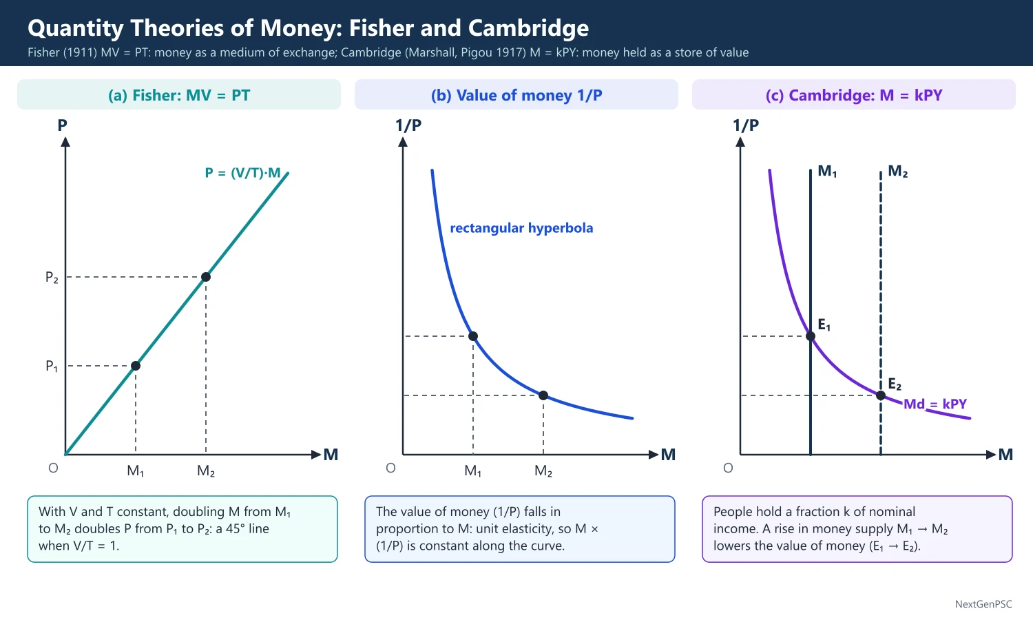
The quantity theory of money links the stock of money to the price level. Fisher's transactions version (MV = PT) treats money as a medium of exchange, the Cambridge version of Marshall and Pigou (M = kPY) treats it as a store of value people choose to hold, and Milton Friedman's 1956 restatement turns it into a stable theory of the demand for money. All three predict that, in the long run, money mainly moves prices, not output.
In simple words
The quantity theory of money says that if the amount of money in an economy grows much faster than the goods it produces, prices rise.
Think of a village fair with a fixed number of mangoes: if every buyer suddenly gets double the cash, the mangoes simply sell at about double the price.
This idea explains why printing money to pay bills causes inflation and why central banks watch money growth.
UPSC asks you to compare Fisher, Cambridge and Friedman versions and to say what each assumes.
1. Concepts and Definitions
Quantity theory of money (QTM): the proposition that, other things equal, the price level varies directly and proportionately with the quantity of money; its roots go back to Jean Bodin (1568), John Locke and David Hume (1752).
Velocity of circulation (V): the average number of times a unit of money changes hands in a period in buying goods and services.
Neutrality of money: a change in the money stock changes only nominal variables (prices, nominal wages) and leaves real variables (output, employment, relative prices) unchanged.
Classical dichotomy: the classical separation of the real sector (where relative prices, output and the real interest rate are set) from the monetary sector (where only the absolute price level is set).
Cash-balance (k): the fraction of annual nominal income that people wish to hold as money; k is the reciprocal of income velocity (k = 1/V).
2. Fisher's Transactions Approach
Source: Irving Fisher, The Purchasing Power of Money (1911).
Equation of exchange: MV + M'V' = PT, where M is currency, V its velocity, M' bank (demand) deposits, V' their velocity, P the average price level and T the volume of transactions.
Simple form: MV = PT, so P = MV/T; the equation is an identity (total money spent = total value of goods bought) until assumptions turn it into a theory.
Assumptions: V and V' are fixed in the short run by habits, banking practice and payment systems; T is fixed at full employment (Say's law); M' bears a stable ratio to M; P is passive, an effect and never a cause.
Result: with V and T constant, a 10% rise in M raises P by 10%; the value of money (1/P) falls in proportion.
Transition period: Fisher himself admitted that in the short run (his 'transition periods') a money increase can change interest rates, output and velocity, so strict proportionality is a long-run claim.
3. The Cambridge Cash-Balance Approach
Origin: Alfred Marshall's oral tradition at Cambridge, written up by A.C. Pigou, 'The Value of Money' (Quarterly Journal of Economics, 1917), and by D.H. Robertson and J.M. Keynes, A Tract on Monetary Reform (1923).
Marshall-Pigou equation: M = kPY, where Y is real income and k the proportion of nominal income held as cash; Pigou wrote it as P = kR/M, with P the value of money (purchasing power) and R total real resources.
Keynes' Tract version: n = p(k + rk'), where n is currency, p the price of a consumption unit, k units held as cash, k' units held as bank deposits and r the cash reserve ratio of banks.
Robertson's version: M = PkT, applying k to total transactions rather than income.
Mechanism: if M rises with k and Y given, people hold more money than they want; they spend the excess, which bids up P until M/P again equals kY.
Why it is an advance: it makes money demand a matter of choice (a demand function), points to wealth, interest and expectations as determinants of k, and uses income (Y) which is easier to measure than T.
4. Fisher and Cambridge Compared
Function of money: Fisher stresses medium of exchange (money on the wing), Cambridge stresses store of value (money sitting).
Nature: Fisher's is a flow analysis over a period; Cambridge is a stock analysis at a point of time.
Equivalence: formally k = 1/V (income velocity), so MV = PY and M = kPY are the same if Y replaces T; the economic content differs because k is a behavioural choice while V is a mechanical rate.
Shared weakness: both assume full employment and a stable k or V, and neither integrates the rate of interest, which Keynes later made central.
5. Friedman's Modern Quantity Theory
Source: Milton Friedman, 'The Quantity Theory of Money: A Restatement', in Studies in the Quantity Theory of Money (1956); evidence in Friedman and Anna Schwartz, A Monetary History of the United States, 1867–1960 (1963).
Key claim: the quantity theory is in the first instance a theory of the demand for money, not of output, prices or income.
Demand function: Md/P = f(Yp, w; rm, rb, re, (1/P)(dP/dt); u), where Yp is permanent income (wealth proxy), w the ratio of non-human to human wealth, rm the return on money, rb on bonds, re on equities, (1/P)(dP/dt) the expected inflation rate (return on goods) and u tastes.
Money as an asset: money is one way of holding wealth, like a durable consumer good yielding a flow of services; demand depends on total wealth and returns on rival assets.
Stability: the demand function is stable and interest-inelastic, so velocity is predictable (not constant); hence changes in M lead to predictable changes in nominal income.
Short run versus long run: money changes affect real output in the short run with 'long and variable lags'; in the long run they affect only prices; hence the famous claim (Friedman, 1963) that inflation is always and everywhere a monetary phenomenon.
Policy rule: because lags are long and variable, Friedman favoured a fixed rule of steady money growth (about 3–5% a year) over discretion (A Program for Monetary Stability, 1960).
6. Criticisms and Limitations
Keynes' critique: in The General Theory (1936) Keynes argued that below full employment a rise in M can raise output, that V is unstable, and that the link from M to P runs through the rate of interest and effective demand.
Velocity instability: financial innovation (credit cards, money market funds, digital payments such as UPI in India) has made velocity unstable; the US and UK abandoned monetary targets in the 1980s for this reason.
Causation: post-Keynesians (Kaldor, Moore) argue money is endogenous: prices and output drive bank lending and money, not the reverse (reverse causation).
Identity, not theory: MV = PT holds by definition; its predictive power depends wholly on the constancy assumptions.
Neglect of the real balance and interest channels: Patinkin, Money, Interest and Prices (1956), showed that the classical dichotomy is logically inconsistent and integrated money through the real balance effect.
7. Diagrams to Draw
Fisher's P–M line: draw M on the horizontal axis and P on the vertical; draw a straight line from the origin at 45° (P = M when V/T = 1), showing that doubling M from M1 to M2 doubles P from P1 to P2.
Value of money curve: plot 1/P on the vertical axis and M on the horizontal; draw a rectangular hyperbola, showing unit elasticity of the value of money with respect to M.
Cambridge demand curve: put M on the horizontal axis and 1/P on the vertical; the demand for money, kY, is a rectangular hyperbola; draw a vertical money supply line M1 and shift it to M2; the new intersection shows the lower value of money.
Friedman's lag diagram (optional): draw time on the horizontal axis; plot money growth peaking first and nominal income growth peaking several quarters later to show long and variable lags.
8. Examples and Applications
India: RBI's monetary targeting from 1985 to 1998, based on the Sukhamoy Chakravarty Committee (1985), used the QTM logic: target M3 growth = expected real GDP growth + tolerable inflation − expected change in velocity.
Hyperinflations: Germany 1923, Zimbabwe 2007–08 and Venezuela after 2016 show prices exploding with money printing, the strongest support for the QTM in extreme cases.
Long-run cross-country evidence: studies covering many countries (for example McCandless and Weber, 1995) find a correlation close to one between long-run money growth and inflation.
Counter-example: after 2008 the US, euro area and Japan expanded base money massively through quantitative easing with low inflation for years, as velocity and the money multiplier fell.
9. Using it in the Exam
10 marks (150 words): define QTM, write MV = PT and M = kPY, state the key assumptions and one point of difference.
15 marks (200 words): add the Fisher versus Cambridge comparison table and one diagram (45° line or rectangular hyperbola).
20 marks (250 words): Fisher, Cambridge, Friedman's demand function and its stability claim, Keynes' critique, and an Indian illustration (monetary targeting 1985–98, shift to inflation targeting in 2016).
Keywords: equation of exchange, velocity, cash balance k, neutrality, classical dichotomy, permanent income, stable demand function, long and variable lags.
Quotation: 'Inflation is always and everywhere a monetary phenomenon' – Milton Friedman.
| Feature | Fisher (1911) | Cambridge (Marshall, Pigou 1917) | Friedman (1956) |
|---|---|---|---|
| Equation | MV = PT | M = kPY | Md/P = f(Yp, w, rm, rb, re, expected inflation, u) |
| Function of money stressed | Medium of exchange | Store of value | Asset among many forms of wealth |
| Key variable | Velocity V (mechanical) | Cash balance k (choice) | Permanent income and asset returns |
| Nature of analysis | Flow, over a period | Stock, at a point of time | Portfolio demand, stable function |
| Role of interest rate | Ignored | Mentioned, not formalised | Included but weak effect |
| Prediction | P proportional to M | P proportional to M (k given) | Money affects output in short run, prices in long run |
Mains points
- Show that MV = PT is an identity and becomes a theory only with assumptions about V and T; examiners reward this distinction.
- Prove equivalence of the two versions (k = 1/V) and then explain why the Cambridge version is still considered superior.
- For Friedman, write the full demand function and state that he restated the QTM as a theory of money demand, not of prices.
- Bring in Keynes' critique (unemployment, unstable velocity, interest rate link) and Patinkin's real balance effect for balance.
- Indian angle: monetary targeting 1985–98 (Chakravarty Committee), multiple indicator approach 1998, flexible inflation targeting from 2016.
- Common mistake: saying Friedman assumed constant velocity; he assumed a stable, predictable demand function.
- Draw at least one diagram; a 45° P–M line or the rectangular hyperbola earns marks quickly.
Did you know?
- Memory trick: Fisher's money 'flies' (money on the wing), Cambridge money 'sits' (money sitting), and Friedman's money is 'one asset in a portfolio'.
Keynes and Post-Keynesian Theories of Demand for Money
Keynes, in The General Theory (1936), explained why people hold money through three motives: transactions, precautionary and speculative, giving L = L1(Y) + L2(r). The speculative motive makes money demand depend on the rate of interest and creates the possibility of a liquidity trap. Post-Keynesians refined it: Baumol (1952) and Tobin (1956) showed that even transactions demand is interest-elastic (the square-root rule), and Tobin (1958) explained speculative demand as diversification by risk-averse investors.
In simple words
Why keep cash at all when a bank fixed deposit or a bond pays interest? Keynes called this preference for cash liquidity preference.
You keep some cash for daily bills, some for emergencies like a hospital visit, and some waiting for a better chance to buy bonds or shares.
Because holding cash means giving up interest, people hold less money when interest rates are high, which links money to interest rates and policy.
UPSC asks you to explain the three motives, the liquidity trap and the Baumol-Tobin model with diagrams.
1. Concepts and Definitions
Liquidity preference: Keynes' term for the desire to hold wealth in the form of money, the most liquid asset; interest is the reward for parting with liquidity for a specified period (Keynes, The General Theory, 1936, chapters 13 and 15).
Transactions motive: money held to bridge the gap between receipt of income and payments; depends mainly on income and on the payment interval.
Precautionary motive: money held for unforeseen expenses and unexpected opportunities; Keynes made it depend on income too.
Speculative motive: money held to profit from knowing better than the market what the future will bring, that is, to avoid capital losses on bonds when interest rates are expected to rise.
Liquidity trap: a situation at a very low interest rate where everyone expects rates to rise (bond prices to fall), so the demand for money becomes perfectly elastic and extra money is simply hoarded; Keynes mentioned the possibility, the term was popularised later by D.H. Robertson and by Hicks' IS-LM work.
2. Keynes' Model Step by Step
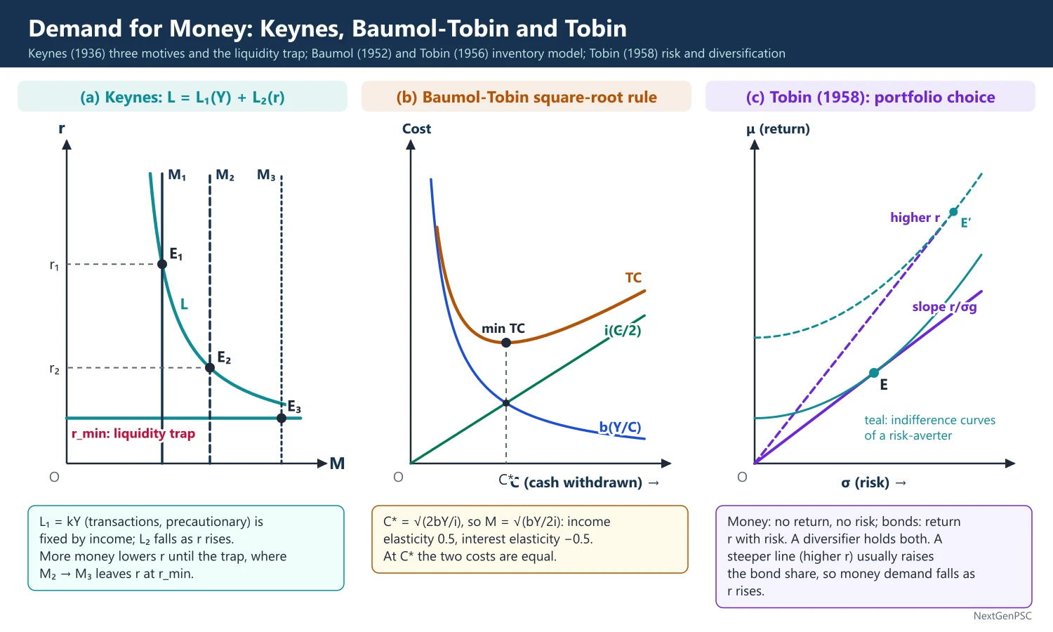
Total demand: L = L1 + L2, where L1 = kY (transactions plus precautionary demand, rising with income) and L2 = f(r) (speculative demand, falling with the interest rate).
Bond price and interest: the price of a perpetual bond (consol) is P_B = C/r, where C is the fixed coupon; so when r rises, bond prices fall and bondholders make capital losses.
Normal rate: each investor holds a view of the 'normal' or safe rate; if the current rate is below it, a rise is expected, so the investor holds money; if above, a fall is expected, so the investor holds bonds.
Critical rate: an investor holds all money when r is below r_c = r_n/(1 + r_n), where r_n is the expected rate, because at that point the expected capital loss just equals the interest earned; individual behaviour is all-or-nothing.
Aggregation: because investors differ in their normal rates, aggregate speculative demand is a smooth downward-sloping curve.
Equilibrium interest: r is set where total money demand L equals the money supply M fixed by the central bank; interest is a monetary phenomenon, not the classical reward for saving.
Comparative statics: a rise in M lowers r (along the liquidity preference curve); a rise in Y shifts L1 and the total demand curve right and raises r; in the liquidity trap a rise in M leaves r unchanged.
3. Criticisms of Keynes' Theory
Interest-inelastic transactions demand: Keynes treated L1 as dependent only on income; Baumol and Tobin later showed it also depends on r.
All-or-nothing behaviour: in reality investors hold diversified portfolios of money and bonds, which Keynes' theory cannot explain.
Regressive expectations: the theory needs a fixed normal rate; if expectations adjust to current rates, the speculative demand curve shifts and may disappear in the long run (Tobin's criticism).
Narrow choice of assets: only money and bonds; real assets, equities and other financial assets are ignored (Friedman's criticism).
Empirical evidence: the liquidity trap was rarely observed until Japan in the late 1990s and the advanced economies at the zero lower bound after 2008.
4. Baumol-Tobin Inventory-Theoretic Model
Sources: W.J. Baumol, 'The Transactions Demand for Cash: An Inventory Theoretic Approach' (Quarterly Journal of Economics, 1952); James Tobin, 'The Interest-Elasticity of Transactions Demand for Cash' (Review of Economics and Statistics, 1956).
Assumptions: income Y (in the model often written T) is received at the start of a period and spent evenly; the person keeps the rest in an interest-bearing asset at rate i and withdraws cash C each time at a fixed brokerage cost b.
Cost function: total cost TC = b(Y/C) + i(C/2), the number of withdrawals times b plus the interest forgone on the average cash balance C/2.
Optimisation: setting dTC/dC = 0 gives C* = √(2bY/i), so average money holding M = C*/2 = √(bY/2i).
Square-root rule: the income elasticity of money demand is 0.5 and the interest elasticity is −0.5; there are economies of scale in cash holding, so money demand rises less than in proportion to income.
Implications: transactions demand is interest-elastic; a doubling of all prices (b and Y) doubles nominal money demand, so there is no money illusion; and lower transaction costs (ATMs, UPI, online banking) reduce money demand.
5. Tobin's Portfolio Theory of Speculative Demand
Source: James Tobin, 'Liquidity Preference as Behavior Towards Risk' (Review of Economic Studies, 1958).
Idea: money has zero return but no risk; bonds have an expected return r but risky capital gains or losses; a risk-averse investor chooses a mix of both, so diversification replaces Keynes' all-or-nothing choice.
Opportunity locus: expected return μ = α·r and risk σ = α·σ_g, where α is the share of bonds and σ_g the standard deviation of capital gains; this gives a straight line from the origin in (σ, μ) space with slope r/σ_g.
Effect of a rise in r: the opportunity line becomes steeper; the substitution effect raises bond holding, the income effect can lower it; if the substitution effect dominates, money demand falls as r rises, giving a downward-sloping speculative demand without regressive expectations.
Types of investors: Tobin distinguished risk lovers, plungers (all bonds or all money) and diversifiers; diversifiers explain the observed mixed portfolios.
6. Other Post-Keynesian Refinements
Precautionary demand: E.L. Whalen (1966) modelled precautionary balances as rising with the variance of net payments and the cost of illiquidity, and falling with the interest rate.
Miller-Orr model (1966): firms let cash float between a lower limit and an upper limit and return it to a target point; the optimal spread rises with the variance of cash flows and transaction costs and falls with the interest rate.
Friedman's restatement (1956): treats money as one asset among many; often presented as a reformulation of the quantity theory but closer in method to the Keynesian portfolio approach (a point made by Patinkin and others; debated).
Post-Keynesian endogenous money: Kaldor and Basil Moore, Horizontalists and Verticalists (1988), argue that the central bank sets the interest rate and supplies whatever money is demanded at that rate.
7. Diagrams to Draw
Liquidity preference curve: draw r on the vertical axis and the quantity of money on the horizontal; draw L1 as a vertical line at kY; draw L2 sloping down and becoming horizontal at a low rate r_min (the liquidity trap); add them to get total L.
Money market equilibrium: draw a vertical money supply line M1 cutting L at E1 with rate r1; shift it to M2 to show a lower rate r2; then shift M again within the flat part to show no change in r (the liquidity trap).
Income shift: show L shifting right from L(Y1) to L(Y2) when income rises, raising r at a given M.
Baumol-Tobin cost curves: draw C on the horizontal axis and cost on the vertical; the brokerage cost b(Y/C) is a falling rectangular hyperbola, the interest cost i(C/2) a rising straight line; their sum is U-shaped with a minimum at C* where the two costs are equal.
Tobin's portfolio diagram: upper panel, σ on the horizontal and μ on the vertical, with the opportunity line from the origin and convex indifference curves of a risk-averter touching it; lower panel, σ against the bond share α, showing the share of bonds and money chosen; rotate the line upward to show a rise in r.
8. Examples and Applications
Liquidity trap: Japan from the late 1990s, and the US, UK and euro area after 2008, when policy rates near zero made conventional monetary policy weak and led to quantitative easing and forward guidance.
India and payment technology: the spread of UPI (launched 2016) and digital payments lowers the brokerage cost b in the Baumol-Tobin sense, which predicts lower transactions demand for cash; yet currency in circulation in India rebounded after demonetisation (November 2016), showing that cash demand also has precautionary and informal-economy motives.
COVID-19 shock (2020): households across countries increased cash and bank deposit holdings, a clear rise in precautionary demand for money.
9. Using it in the Exam
10 marks: the three motives, L = L1(Y) + L2(r), and the liquidity trap with a one-line diagram description.
15 marks: add the bond price–interest link and the normal rate argument, plus the liquidity preference diagram.
20 marks: Keynes, then the Baumol-Tobin square-root rule with derivation, Tobin's portfolio theory, and an assessment (empirical stability of money demand, financial innovation, Japan and 2008).
Keywords: liquidity preference, speculative motive, normal rate, liquidity trap, square-root rule, economies of scale, risk aversion, diversification.
Definition to quote: Keynes described interest as the reward for parting with liquidity for a specified period.
| Theory | Motive explained | Determinants | Key result |
|---|---|---|---|
| Keynes (1936) | Transactions, precautionary, speculative | Y for L1; r and normal rate for L2 | Liquidity trap; interest is a monetary phenomenon |
| Baumol (1952), Tobin (1956) | Transactions | Y, i, brokerage cost b | M = √(bY/2i); income elasticity 0.5, interest elasticity −0.5 |
| Tobin (1958) | Speculative (asset) | r, risk σ, risk aversion | Diversified portfolios; downward slope without regressive expectations |
| Friedman (1956) | Money as one asset | Permanent income, returns on bonds, equities, goods | Stable, interest-inelastic demand function |
Mains points
- Always connect the speculative motive to the inverse relation between bond prices and interest rates (P_B = C/r); without it the argument is incomplete.
- Explain why individual speculative demand is a step function but aggregate demand is smooth.
- Derive the Baumol-Tobin square-root formula in three lines and state its two elasticities; examiners expect the derivation in 15–20 mark questions.
- Use Tobin (1958) to answer questions on why people hold both money and bonds, and on the slope of the LM curve.
- Discuss the policy relevance of the liquidity trap: monetary policy ineffective, fiscal policy strong; cite Japan and post-2008 experience.
- Common mistake: writing that the liquidity trap means zero money demand; it means infinitely elastic money demand.
- Link financial innovation and digital payments in India to falling transactions demand and unstable velocity.
Did you know?
- Memory trick for the three motives: T-P-S, 'Tea, Pills and Shares': cash for tea (daily transactions), pills (emergencies) and shares (speculation).
Supply of Money and the Money Multiplier
The money supply is the stock of currency with the public plus bank deposits. It is built on high-powered (reserve) money H, created by the central bank, through the money multiplier: M = mH, where m = (1 + c)/(c + r), c being the currency-deposit ratio and r the reserve-deposit ratio. The exogenous view (Friedman-Schwartz, Brunner-Meltzer) treats money as set by the central bank; the endogenous view (Kaldor, Moore) says bank lending creates deposits and the central bank accommodates them.
In simple words
Most money in India is not notes but bank deposits; banks create these deposits when they give loans.
Like a well that refills: the RBI puts in the first bucket of cash (reserve money), and as people deposit and banks lend, the same rupee is counted again and again as deposits.
The number of times reserve money is stretched is the money multiplier; it decides how far RBI actions such as cutting CRR spread through the economy.
UPSC asks you to derive the multiplier, list its determinants and explain India's M0 to M3 measures.
1. Concepts and Definitions
Money supply (M): the total stock of money held by the public (non-bank sector) at a point of time; it excludes money held by the government, the central bank and commercial banks themselves.
High-powered money (H) or reserve money (M0): the monetary liabilities of the central bank: currency held by the public (C) plus reserves of banks (R), which include cash in vaults and deposits with the central bank; it is called high-powered because each rupee of it supports several rupees of deposits.
Currency-deposit ratio (c = C/D): chosen by the public; it rises with distrust of banks, festivals, harvest season, informal activity and falls with financial inclusion and digital payments.
Reserve-deposit ratio (r = R/D): set partly by law (the cash reserve ratio, CRR) and partly by banks' choice of excess reserves.
Money multiplier (m): the ratio of the money stock to high-powered money, m = M/H.
2. Deriving the Money Multiplier
Step 1: M = C + D (currency with the public plus deposits).
Step 2: H = C + R (currency plus bank reserves).
Step 3: divide: M/H = (C + D)/(C + R); divide numerator and denominator by D to get m = (c + 1)/(c + r).
Result: M = [(1 + c)/(c + r)]·H; since r is less than 1, m is greater than 1.
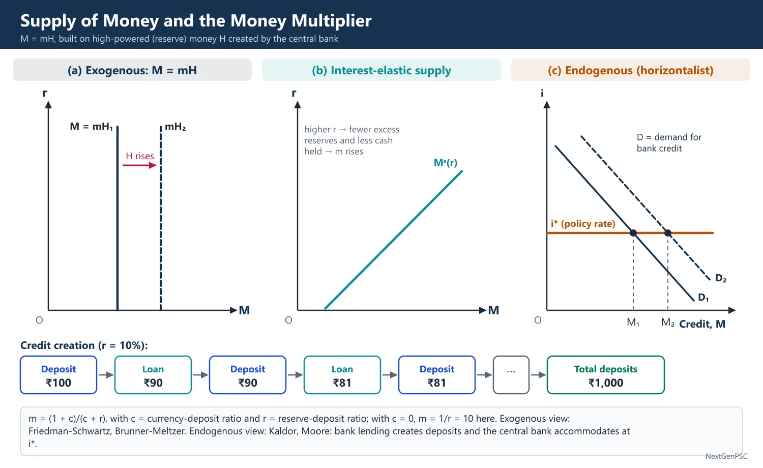
Simple deposit multiplier: if the public holds no currency (c = 0), m = 1/r; with a 10% reserve ratio one rupee of reserves supports ten rupees of deposits.
Comparative statics: ∂m/∂r is negative (a CRR cut raises m); ∂m/∂c is negative when r is less than 1 (more cash holding leaks out of the banking system and lowers m).
Worked example: with c = 0.2 and r = 0.05, m = 1.2/0.25 = 4.8; if CRR falls so that r = 0.04, m = 1.2/0.24 = 5.
3. Credit Creation by Banks
Textbook process: a fresh deposit of ₹100 with r = 10% lets the bank lend ₹90; the borrower spends it, it is redeposited, and the second bank lends ₹81, and so on; total deposits = 100/(1 − 0.9) = ₹1,000.
Leakages: cash drain to the public, excess reserves held by cautious banks, lack of creditworthy borrowers, and statutory liquidity requirements (in India the SLR locks part of deposits in government securities).
Early writers: the idea of deposit creation goes back to H.D. Macleod and was formalised by C.A. Phillips, Bank Credit (1920).
4. Determinants of the Money Supply
Friedman-Schwartz framework (1963): three proximate determinants: high-powered money (central bank), the deposit-reserve ratio (banks) and the deposit-currency ratio (public).
Sources of reserve money in India: net RBI credit to the government, RBI credit to banks and the commercial sector, net foreign exchange assets of the RBI, and government currency liabilities to the public, minus net non-monetary liabilities of the RBI.
Sources of broad money (M3) in India: net bank credit to the government, bank credit to the commercial sector, net foreign exchange assets of the banking sector, government currency liabilities to the public, minus net non-monetary liabilities of the banking sector.
Open-economy link: when the RBI buys dollars to stop the rupee rising, its foreign assets and reserve money rise; it may sterilise this by selling government securities (open market operations, or the Market Stabilisation Scheme introduced in 2004).
Fiscal link: before 1997 automatic monetisation through ad hoc Treasury bills made government deficits a major source of reserve money; this was ended by the 1994 agreement between the RBI and the government, effective April 1997.
5. Measures of Money in India
Second Working Group on Money Supply (1977): introduced M1 to M4.
M1 (narrow money): currency with the public + demand deposits with banks + 'other' deposits with the RBI.
M2: M1 + savings deposits with post office savings banks.
M3 (broad money): M1 + time deposits with banks; the main monetary aggregate used by the RBI.
M4: M3 + total post office deposits (excluding National Savings Certificates).
Working Group on Money Supply: Analytics and Methodology of Compilation (1998): chaired by Y.V. Reddy, introduced new aggregates NM1, NM2 and NM3 (NM2 includes short-term time deposits up to one year) and liquidity aggregates L1, L2, L3 that include post office deposits and deposits with financial institutions.
Liquidity order: M1 is most liquid and M4 least; the M3/M0 ratio is the broad money multiplier.
6. Exogenous versus Endogenous Money
Exogenous (monetarist) view: the central bank controls H and, with a stable multiplier, controls M; associated with Friedman and Schwartz, Karl Brunner and Allan Meltzer, and Phillip Cagan.
Endogenous (post-Keynesian) view: Nicholas Kaldor, The Scourge of Monetarism (1982), and Basil Moore, Horizontalists and Verticalists (1988): banks lend first and find reserves later; the central bank sets the interest rate and must supply reserves on demand to avoid financial instability, so the money supply curve is horizontal at the policy rate.
Bank of England view: the article 'Money creation in the modern economy' (Bank of England Quarterly Bulletin, 2014) stated that commercial banks create most money when they make loans, and that the money multiplier is not a mechanical description of how money is created.
Reconciliation: under an interest-rate operating target (as in India's liquidity adjustment facility since 2000 and the repo-based framework since 2011), money is largely endogenous in the short run; the multiplier identity still holds but its causation runs from demand for credit.
7. Criticisms and Limitations of the Multiplier Approach
Instability of c and r: after 2008 banks in the US held huge excess reserves, so base money tripled but broad money grew slowly; m collapsed.
Behavioural ratios: c and r depend on interest rates, income and confidence, so the multiplier is itself a function, not a constant (Brunner and Meltzer's money supply function).
Ignores non-bank finance: NBFCs, mutual funds and shadow banking create close substitutes for money.
8. Diagrams to Draw
Exogenous money supply: draw r on the vertical axis and M on the horizontal; draw a vertical money supply line at M = mH; show a rise in H shifting it right.
Interest-elastic money supply: draw an upward-sloping money supply curve, because higher interest rates lead banks to hold fewer excess reserves and the public to hold less cash, raising m.
Endogenous (horizontalist) money supply: draw a horizontal line at the policy rate i*; a downward-sloping credit demand curve determines the quantity of money; a rise in credit demand raises M without changing i*.
Credit creation flow chart: draw a chain of boxes, deposit ₹100 → loan ₹90 → deposit ₹90 → loan ₹81 …, ending in total deposits of ₹1,000 for r = 10%.
9. Examples and Applications
Demonetisation (8 November 2016): ₹500 and ₹1,000 notes, about 86% of currency in circulation by value, were withdrawn; c fell sharply, deposits surged, and the money multiplier rose temporarily before currency was remonetised; the RBI reported that about 99% of the withdrawn notes returned.
CRR changes: the RBI cut CRR from 4% to 3% in four steps between September and November 2025, releasing primary liquidity of about ₹2.5 lakh crore and raising the multiplier.
Digital currency: the RBI's e-rupee (CBDC) pilots began in 2022 (wholesale in November, retail in December); wide use could change c and the structure of reserve money.
Quantitative easing: the US Federal Reserve after 2008 shows that a large rise in H need not raise M proportionately when banks hoard reserves.
10. Using it in the Exam
10 marks: define H and m, derive m = (1 + c)/(c + r) and state its determinants.
15 marks: add the sources of reserve money in India and the M1–M4 measures.
20 marks: derivation, determinants, India's measures, the endogenous money critique and a current Indian example (CRR changes, demonetisation, sterilisation).
Keywords: high-powered money, reserve money, currency-deposit ratio, reserve ratio, credit creation, broad money, sterilisation, endogenous money.
Point to quote: Friedman and Schwartz identified three proximate determinants of the money stock: high-powered money, the deposit-reserve ratio and the deposit-currency ratio.
| Measure | Components | Liquidity |
|---|---|---|
| M0 (reserve money) | Currency in circulation + bankers' deposits with RBI + other deposits with RBI | Base of the system |
| M1 (narrow money) | Currency with public + demand deposits with banks + other deposits with RBI | Highest |
| M2 | M1 + savings deposits of post office savings banks | High |
| M3 (broad money) | M1 + time deposits with banks | Lower; main policy aggregate |
| M4 | M3 + total post office deposits (excluding NSCs) | Lowest |
Mains points
- Write the derivation in four lines (M = C + D, H = C + R, divide by D, m = (1 + c)/(c + r)); a derivation is expected even in 10-mark parts.
- Classify determinants by who controls them: central bank (H, CRR), banks (excess reserves), public (c).
- Explain the sources of reserve money in India; questions often ask how RBI forex intervention or government borrowing affects money supply.
- Add the endogenous money critique (Kaldor, Moore, Bank of England 2014) to show analytical depth.
- Common mistake: treating SLR as part of the multiplier formula; in the basic formula r is the cash reserve ratio plus excess reserves, while SLR affects credit available to the private sector.
- Use demonetisation 2016 and CRR changes as Indian illustrations of shifts in c and r.
Did you know?
- Banks lend money they never received as cash: in India broad money (M3) is several times reserve money, so most of the 'money' people hold exists only as entries in bank ledgers.
Goals and Instruments of Monetary Policy in Closed and Open Economies
Monetary policy is the central bank's control of money, credit and interest rates to achieve price stability, growth and employment, external balance and financial stability. It works through quantitative instruments (policy rate, open market operations, reserve ratios) and qualitative instruments (selective credit controls, moral suasion). In an open economy capital flows and the exchange rate add channels and constraints: a country cannot have a fixed exchange rate, free capital mobility and an independent monetary policy at the same time (the impossible trinity).
In simple words
Monetary policy is how the RBI changes interest rates and the amount of money to keep prices stable and the economy growing.
It is like the accelerator and brake of a car: cutting the repo rate presses the accelerator (cheaper loans), raising it presses the brake (to cool inflation).
In an open economy foreign money flows in and out, so the RBI must also watch the rupee and its forex reserves.
UPSC asks you to list goals and instruments, explain conflicts between goals and discuss how openness limits policy.
1. Concepts and Definitions
Monetary policy: the use by the monetary authority of instruments under its control (interest rates, reserves, credit) to influence aggregate demand, prices and financial conditions.
Goals (ultimate objectives): price stability, high growth and employment, balance of payments equilibrium, exchange rate stability and financial stability.
Targets and indicators: operating targets the central bank controls daily (in India the weighted average call rate, WACR), intermediate targets linked to goals (money supply, interest rates, exchange rate or the inflation forecast), and final goals.
Tinbergen rule: Jan Tinbergen, On the Theory of Economic Policy (1952): to achieve n independent targets a government needs at least n independent instruments.
Mundell's assignment principle: Robert Mundell (1962): each instrument should be assigned to the target on which it has the greatest relative effect (the principle of effective market classification).
2. Goals and the Conflicts among Them
Price stability versus growth: the short-run Phillips curve (A.W. Phillips, 1958) implies a trade-off between inflation and unemployment; Friedman (1968) and Phelps (1967) argued the trade-off vanishes in the long run (vertical long-run Phillips curve at the natural rate).
Internal versus external balance: a tight policy to cut inflation may attract capital inflows and appreciate the currency, hurting exports; a loose policy to support growth may widen the current account deficit.
Price stability versus financial stability: low inflation can coexist with asset bubbles (US housing before 2008), so many central banks now add macroprudential tools.
Modern consensus: make price stability the primary goal through flexible inflation targeting, while giving weight to growth (Svensson's 'flexible' inflation targeting); India adopted this in 2016.
3. Quantitative (General) Instruments
Bank rate: the rate at which the central bank rediscounts bills or lends to banks; Henry Thornton and the Bank of England's 19th-century practice made it the classic tool; in India it is now aligned to the MSF rate.
Policy (repo) rate: the rate at which the RBI lends overnight to banks against government securities under the liquidity adjustment facility (LAF, introduced 2000); it is decided by the Monetary Policy Committee.
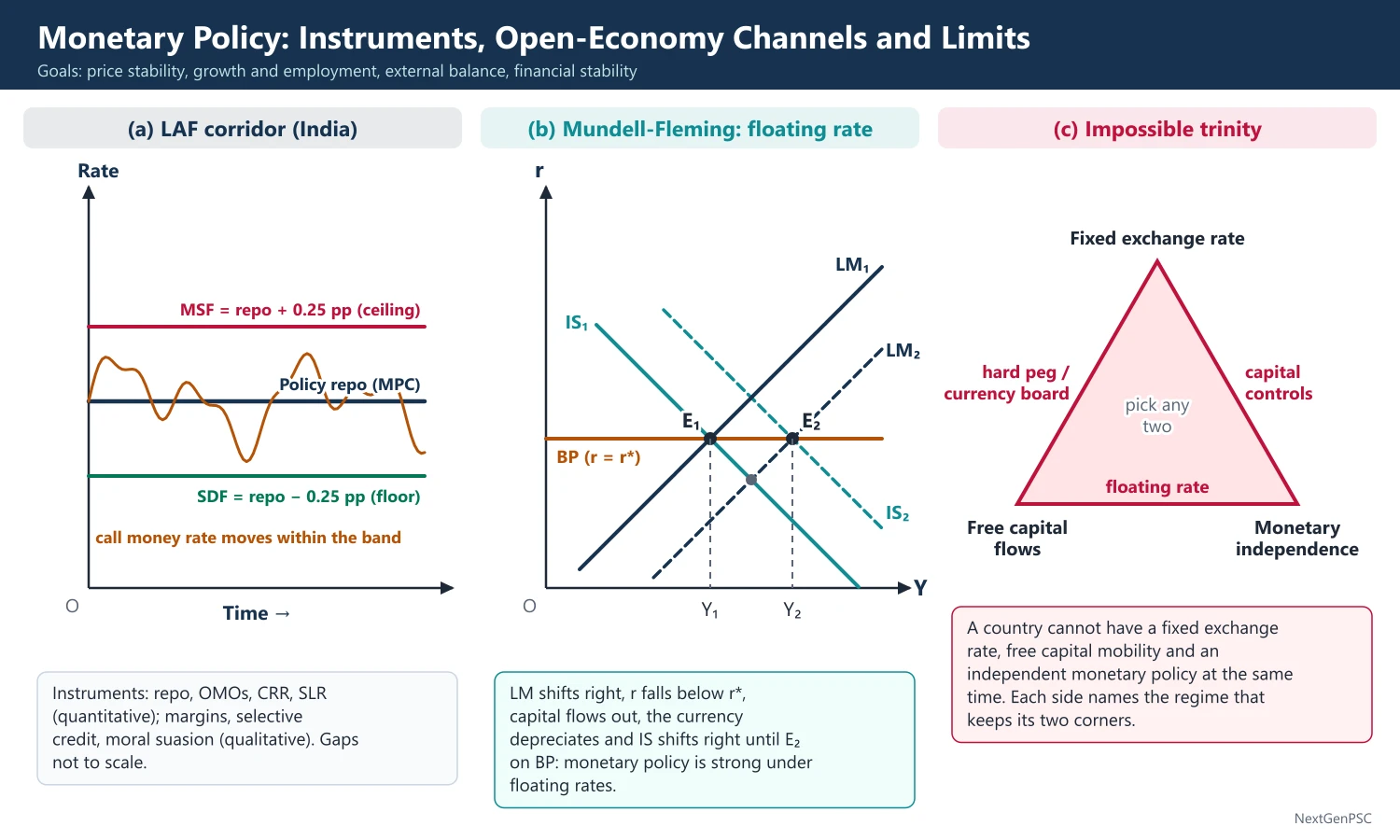
Corridor: the Standing Deposit Facility (SDF, introduced April 2022, a collateral-free absorption window) forms the floor and the Marginal Standing Facility (MSF, 2011) the ceiling, each 25 basis points from the repo rate.
Open market operations (OMOs): outright purchase or sale of government securities to inject or absorb durable liquidity; variable rate repo and reverse repo auctions manage short-term liquidity.
Cash reserve ratio (CRR): share of net demand and time liabilities banks must keep with the RBI (Section 42 of the RBI Act, 1934); unremunerated.
Statutory liquidity ratio (SLR): share of deposits banks must hold in liquid assets such as government securities (Section 24 of the Banking Regulation Act, 1949).
Market Stabilisation Scheme (2004): issue of special government securities to sterilise the liquidity created by forex purchases.
4. Qualitative (Selective) Instruments
Margin requirements: the share of a loan's collateral value that cannot be lent; raised to curb speculative lending against shares or commodities.
Selective credit controls: ceilings or higher costs on credit for particular sectors or commodities (used in India for sensitive commodities such as foodgrains and sugar in the past).
Directed credit: priority sector lending targets (40% of adjusted net bank credit for domestic scheduled commercial banks), which channel credit to agriculture, MSMEs and weaker sections.
Moral suasion and direct action: persuasion through meetings and letters; penalties or restrictions on banks that do not comply.
Macroprudential tools: higher risk weights, countercyclical capital buffers and loan-to-value limits, used by the RBI on consumer credit and NBFC lending (for example the higher risk weights of November 2023).
5. Transmission Channels
Interest rate channel: policy rate → money market rates → bank lending and deposit rates → investment and consumption (the Keynesian channel of IS-LM).
Credit channel: Ben Bernanke and Mark Gertler (1995), Bernanke and Blinder (1988): tight money reduces bank loan supply (bank lending channel) and weakens borrowers' balance sheets (balance sheet channel).
Asset price channel: lower rates raise share and property prices, raising Tobin's q (investment) and household wealth (consumption).
Exchange rate channel: in an open economy a rate cut lowers returns on domestic assets, the currency depreciates, net exports rise and imported inflation rises.
Expectations channel: credible commitments and forward guidance shape inflation expectations and long-term rates.
Lags: Friedman's inside lag (recognition and decision) and outside lag (effect on the economy); the RBI's estimates suggest the full effect on inflation takes several quarters.
India's transmission reforms: Base Rate (2010), Marginal Cost of Funds based Lending Rate (MCLR, April 2016), and the external benchmark-based lending rate (EBLR, October 2019) linking new floating-rate retail and MSE loans to the repo rate or similar benchmarks.
6. Choice of Target: Money or Interest Rate
William Poole (1970): in an IS-LM model with shocks, if money demand (LM) shocks dominate, an interest rate target stabilises output better; if spending (IS) shocks dominate, a money supply target is better.
Practice: most central banks moved from money targets (1970s–80s) to interest rate operating targets as money demand became unstable with financial innovation; India moved from monetary targeting (1985–98) to a multiple indicator approach (1998) and to flexible inflation targeting (2016).
7. Monetary Policy in an Open Economy
Impossible trinity (trilemma): from the Mundell-Fleming model: a country can choose only two of fixed exchange rate, free capital mobility and monetary autonomy.
Sterilised intervention: the central bank buys foreign exchange (raising reserve money) and sells domestic bonds to absorb the extra liquidity; costly because domestic interest exceeds returns on reserves (quasi-fiscal cost) and hard to sustain under large inflows.
Mundell-Fleming results: with perfect capital mobility, monetary policy is powerful under floating exchange rates (through depreciation and net exports) and powerless under fixed rates (any money expansion leaks out as reserves fall).
Global spillovers: Hélène Rey (2013) argued that a global financial cycle driven by US monetary policy reduces the trilemma to a 'dilemma' for open economies: independent policy is possible only with capital flow management.
India's middle path: a managed float, partial capital account convertibility, large forex reserves and inflation targeting; the RBI intervenes to curb excess volatility, not to defend a level.
8. Diagrams to Draw
IS-LM closed economy: draw IS sloping down and LM sloping up in (Y, r) space; an expansionary monetary policy shifts LM to the right, lowering r and raising Y; show the weak effect when LM is flat (liquidity trap) and the strong effect when IS is flat.
LAF corridor: draw time on the horizontal axis and interest rate on the vertical; draw three horizontal lines, MSF at the top, repo in the middle, SDF at the bottom; plot the call money rate moving within the band.
Mundell-Fleming under floating rates: draw IS, LM and a horizontal BP line at the world rate r*; an LM shift right lowers r below r*, capital flows out, the currency depreciates, IS shifts right until it meets the new LM on the BP line at a higher Y.
Impossible trinity triangle: draw a triangle with vertices labelled fixed exchange rate, free capital flows and monetary independence; mark each side with the regime that results (for example, side between free capital and monetary independence = floating rate).
9. Examples and Applications
India 2022–23: the MPC raised the repo rate from 4.0% (May 2022) to 6.5% (February 2023) to bring CPI inflation back towards target.
India 2025–26: with inflation low, the repo rate was cut from 6.5% to 5.5% between February and June 2025 and to 5.25% in December 2025, and CRR was cut to 3% in steps up to November 2025; on 7 October 2026 the MPC raised it to 5.50% and moved its stance to calibrated tightening.
Taper tantrum (2013): the US Federal Reserve's signal of reduced bond purchases caused capital outflows and a sharp rupee fall; the RBI used higher short-term rates, swap windows and FCNR(B) deposit schemes.
2007–08 inflows: large capital inflows forced the RBI to buy dollars and sterilise through the MSS and CRR increases, a classic trilemma case.
10. Using it in the Exam
10 marks: list goals and classify instruments (quantitative and qualitative) with one Indian example each.
15 marks: add goal conflicts (Phillips curve, internal versus external balance) and transmission channels.
20 marks: closed versus open economy contrast with the impossible trinity, sterilisation, Mundell-Fleming results and India's managed float plus inflation targeting.
Keywords: Tinbergen rule, repo rate, LAF corridor, OMO, CRR, SLR, transmission, sterilisation, trilemma, flexible inflation targeting.
Statement to quote: Tinbergen's rule that the number of instruments must at least equal the number of targets.
| Aspect | Closed economy | Open economy |
|---|---|---|
| Goals | Price stability, growth, employment | Also BoP equilibrium and exchange rate stability |
| Channels | Interest rate, credit, asset prices | Adds exchange rate and capital flow channels |
| Constraint | Liquidity trap, lags | Impossible trinity; global financial cycle |
| Source of reserve money | Mainly credit to government and banks | Also net foreign assets; needs sterilisation |
| Effectiveness (Mundell-Fleming, perfect capital mobility) | Depends on IS and LM slopes | Strong under floating, weak under fixed rates |
| Rate | Relation to repo | Role |
|---|---|---|
| MSF rate and Bank Rate | Repo + 0.25 percentage point | Ceiling; emergency borrowing by banks |
| Policy repo rate | Set by MPC | Signals the stance of policy |
| Standing Deposit Facility (since April 2022) | Repo − 0.25 percentage point | Floor; absorbs surplus liquidity without collateral |
Mains points
- Structure answers as goals → targets → instruments → channels → constraints; this sequence signals mastery.
- Explain at least one goal conflict with a diagram (short-run Phillips curve, or internal versus external balance).
- For open economies, the impossible trinity and sterilisation are almost always expected; add its costs (quasi-fiscal cost, rising interest rates).
- Use current Indian instruments correctly: SDF as floor since April 2022, MSF ceiling, CRR under Section 42, EBLR from October 2019.
- Add Poole's (1970) analysis when asked about the choice between money and interest rate targets.
- Common mistake: calling CRR a qualitative instrument; it is quantitative (general), while margin requirements and moral suasion are qualitative.
- Conclude with the modern consensus of flexible inflation targeting plus macroprudential policy.
Did you know?
- Memory trick for the trilemma: 'You can have any two of the three F's: Fixed rate, Free capital, Free (independent) monetary policy.'
Central Bank and Treasury; Rules versus Discretion and Money Growth Ceilings
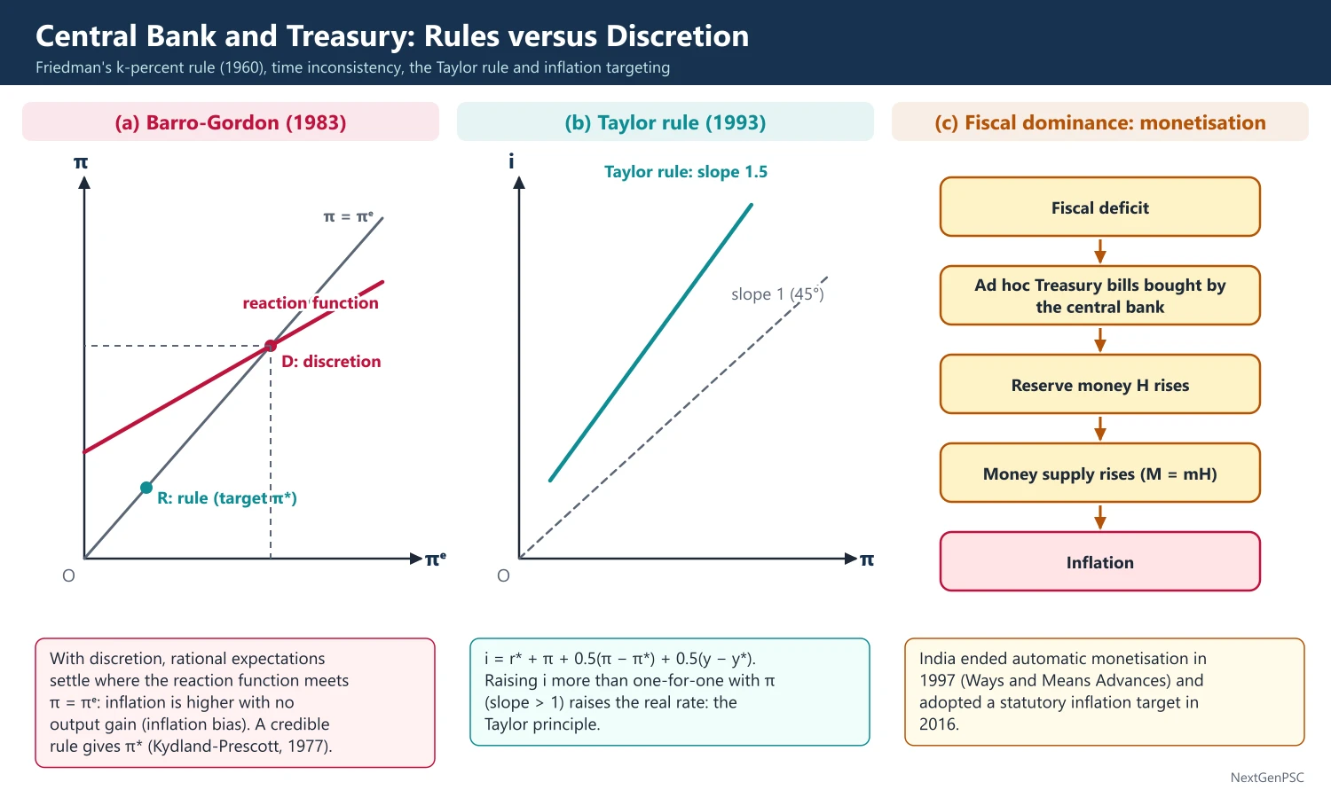
The relation between the central bank and the treasury decides whether monetary policy can control inflation: when deficits are automatically financed by the central bank, money supply follows the budget (fiscal dominance). The rules versus discretion debate asks whether policy should follow a fixed rule, such as Friedman's k-percent money growth ceiling or the Taylor rule, or be left to judgement; Kydland and Prescott (1977) and Barro and Gordon (1983) showed that discretion creates an inflation bias. India ended automatic monetisation in 1997 and adopted a statutory inflation target in 2016.
In simple words
The government (treasury) spends and borrows; the central bank controls money. If the government can simply ask the central bank to print money for its deficit, prices rise.
It is like giving a teenager a credit card with no limit: rules such as a fixed spending cap protect against temptation.
So economists debate fixed rules (grow money by a set percent) versus letting the central bank use judgement.
UPSC asks about central bank independence, Friedman's money growth rule and India's shift from ad hoc treasury bills to inflation targeting.
1. Concepts and Definitions
Monetisation of deficit: financing a government deficit by borrowing from the central bank, which creates reserve money.
Fiscal dominance: a regime in which fiscal policy is set first and monetary policy must accommodate it; the opposite is monetary dominance.
Central bank independence: the freedom of the central bank to set its instruments (instrument independence) and sometimes its goals (goal independence) without government direction; in India the government sets the inflation target and the RBI has instrument independence.
Rule: a pre-announced formula for setting the policy instrument (for example money growth of k% a year); discretion: period-by-period choice of the best policy given current conditions.
Time inconsistency: a policy that is optimal when announced ceases to be optimal later, so a rational policymaker will deviate, and rational agents anticipate it (Finn Kydland and Edward Prescott, 'Rules Rather than Discretion', Journal of Political Economy, 1977).
2. Central Bank and Treasury: Theory
Government budget constraint: G − T = ΔB + ΔH, where ΔB is new bonds sold to the public and ΔH new reserve money; any deficit not covered by bonds must be monetised.
Seigniorage and inflation tax: the real revenue from money creation, ΔH/P = (ΔH/H)·(H/P); beyond a point higher money growth reduces real balances so much that revenue falls (Phillip Cagan, 1956, study of hyperinflations).
Sargent and Wallace, 'Some Unpleasant Monetarist Arithmetic' (1981): if fiscal policy is dominant and debt cannot grow faster than the economy indefinitely, tight money today means more debt and more monetisation later, so tight money can even raise inflation; monetary control requires fiscal discipline.
Fiscal theory of the price level: Leeper (1991), Sims and Woodford argued that the price level adjusts to make the real value of government debt equal the present value of surpluses (debated).
Conflict of debt management: as debt manager, the central bank wants low interest rates on government debt; as inflation fighter, it may need high rates; hence proposals to move debt management out of the central bank.
3. Central Bank and Treasury in India
RBI Act, 1934: the RBI is banker and debt manager to the Central Government (Sections 20 and 21) and to states by agreement (Section 21A); Section 7 allows the government to give directions to the RBI after consultation, in the public interest.
Ad hoc Treasury bills (1955–1997): the Centre automatically replenished its cash balance by issuing ad hoc bills to the RBI at a low rate (4.6%), leading to large monetisation in the 1980s.
Sukhamoy Chakravarty Committee (1985): recommended monetary targeting and coordination between fiscal and monetary policy, with limits on RBI credit to government.
1994 agreement: the Government and the RBI agreed in September 1994 to phase out ad hoc bills by 1997; from 1 April 1997 they were replaced by Ways and Means Advances (WMA) with limits.
FRBM Act, 2003: barred the RBI from subscribing to primary issues of central government securities from 1 April 2006, except in specified circumstances (for example under the escape clause).
RBI Act amendment (Finance Act, 2016): Section 45ZA lets the government set the inflation target in consultation with the RBI, Section 45ZB creates a six-member Monetary Policy Committee (three from the RBI including the Governor, who has a casting vote, and three appointed by the government).
Inflation target: 4% CPI with a band of 2% to 6%, first for 2016–21, retained for 2021–26 and, by notification of 25 March 2026, for 1 April 2026 to 31 March 2031.
Surplus transfer: the Bimal Jalan Committee (2019) set the economic capital framework that governs how much RBI surplus goes to the government; the RBI transferred about ₹2.69 lakh crore for 2024–25.
Debt management debate: the 2015–16 Budget proposed a Public Debt Management Agency; it has not been set up, and the RBI continues to manage government debt.
4. Rules versus Discretion
Early rule advocates: Henry Simons, 'Rules versus Authorities in Monetary Policy' (1936), proposed a fixed rule to reduce uncertainty.
Friedman's k-percent rule: Milton Friedman, A Program for Monetary Stability (1960), proposed that the money stock grow at a constant rate (about 3–5% a year, roughly the trend growth of real output), regardless of the cycle; this is the 'ceiling on the growth rate of money' in the syllabus.
Case for the money rule: long and variable lags make fine-tuning destabilising; a rule prevents political pressure and inflationary monetisation; it anchors expectations.
Barro-Gordon model (1983): the policymaker's loss L = a(π − π*)² − b(π − πᵉ) (or a gap-based variant); under discretion, the temptation to create surprise inflation leads to equilibrium inflation above target with no output gain (inflation bias); a credible rule removes the bias.
Solutions to inflation bias: rules, reputation in repeated games, a conservative central banker who weights inflation more (Kenneth Rogoff, 1985), and performance contracts for central bankers (Carl Walsh, 1995).
Taylor rule (John Taylor, 1993): i = r* + π + 0.5(π − π*) + 0.5(y − y*), where r* is the neutral real rate and (y − y*) the output gap; the Taylor principle requires the nominal rate to rise more than one-for-one with inflation.
Constrained discretion: Ben Bernanke and Frederic Mishkin (1997) described inflation targeting as a framework that combines a firm long-run commitment with short-run flexibility.
Case for discretion: shocks are varied (supply shocks, pandemics, financial crises); a rigid rule cannot respond to them, as shown by the large emergency actions of 2008 and 2020.
5. Criticisms of the Money Growth Ceiling
Unstable velocity: financial innovation made money demand unstable in the 1980s, so money targets gave misleading signals; the US Federal Reserve abandoned money targets after the 1979–82 experiment.
Goodhart's law (Charles Goodhart, 1975): paraphrased, any statistical regularity tends to break down once it is used as a target for control.
Lucas critique (1976): policy rules change behaviour, so relations estimated under old policy may not hold under the new rule.
Endogenous money: post-Keynesians argue the central bank cannot control broad money directly, only the interest rate.
India's experience: under monetary targeting (1985–98) M3 targets were often overshot because of fiscal deficits; the RBI moved to a multiple indicator approach in April 1998 because financial liberalisation made money demand less predictable.
6. Diagrams to Draw
Barro-Gordon diagram: draw expected inflation πᵉ on the horizontal axis and actual inflation π on the vertical; draw a 45° line (π = πᵉ) and the policymaker's reaction function sloping up but flatter than 45°; the discretionary equilibrium is where they cross, at inflation above the target; the rule equilibrium is at the target on the 45° line.
Short-run and long-run Phillips curves: draw unemployment on the horizontal axis and inflation on the vertical; show a short-run curve and a vertical long-run curve at the natural rate; a surprise inflation moves along the short-run curve temporarily, then expectations shift it up.
Taylor rule line: draw inflation on the horizontal axis and the policy rate on the vertical; a line steeper than 45° (slope 1.5) satisfies the Taylor principle.
Monetisation flow chart: fiscal deficit → ad hoc T-bills → reserve money rises → money supply rises (M = mH) → inflation.
7. Examples and Applications
India: monetised deficits in the 1980s contributed to inflation and the 1991 crisis; the 1997 WMA system and FRBM 2003 created monetary dominance; during COVID-19 (2020–21) the RBI's large OMO purchases (G-SAP in 2021) were debated as indirect monetisation.
Germany and the Bundesbank: post-war monetary targeting and independence, influenced by the 1923 hyperinflation, shaped the European Central Bank's design (Maastricht Treaty, 1992).
New Zealand: the Reserve Bank of New Zealand Act, 1989, introduced the first formal inflation target, with a policy targets agreement between the Governor and the Finance Minister.
US 1979–82: the Volcker Fed targeted reserves to control money growth, brought inflation down but at the cost of a deep recession and volatile interest rates.
8. Using it in the Exam
10 marks: define fiscal dominance and the k-percent rule; give India's end of ad hoc bills (1997) and FRBM (2006 ban).
15 marks: rules versus discretion with the time-inconsistency argument and the Taylor rule equation.
20 marks: Friedman's case for a money growth ceiling, its criticisms (velocity, Goodhart, Lucas, endogenous money), and India's path from monetary targeting to flexible inflation targeting under the MPC.
Keywords: fiscal dominance, monetisation, seigniorage, ad hoc T-bills, WMA, time inconsistency, inflation bias, conservative central banker, k-percent rule, Taylor rule.
Point to quote: Kydland and Prescott (1977) showed that discretion, even by a benevolent policymaker, can produce worse outcomes than a credible rule.
| Approach | Proponent and year | Rule or idea | Main criticism |
|---|---|---|---|
| Money growth rule | Friedman (1960) | Money stock grows at constant k% (about 3–5%) | Unstable velocity; Goodhart's law |
| Time inconsistency | Kydland-Prescott (1977); Barro-Gordon (1983) | Discretion produces inflation bias; credible rules better | Rules cannot handle unusual shocks |
| Conservative central banker | Rogoff (1985) | Delegate to an inflation-averse banker | Output may become more volatile |
| Interest rate rule | Taylor (1993) | i = r* + π + 0.5(π − π*) + 0.5(y − y*) | Neutral rate and output gap hard to measure |
| Inflation targeting | Bernanke-Mishkin (1997): constrained discretion | Numerical inflation target, flexible in short run | Neglects asset prices and supply shocks |
| Year | Event |
|---|---|
| 1985 | Chakravarty Committee recommends monetary targeting and fiscal-monetary coordination |
| 1994 | Agreement to phase out ad hoc Treasury bills |
| 1997 | Ad hoc bills replaced by Ways and Means Advances (1 April) |
| 2003 / 2006 | FRBM Act; RBI barred from primary subscription to G-secs from 1 April 2006 |
| 2016 | RBI Act amended: inflation target (Section 45ZA) and MPC (Section 45ZB) |
| 2026 | 4% CPI target (2–6% band) notified for 2026–31 |
Mains points
- Interpret 'proposal for a ceiling on the growth rate of money' as Friedman's k-percent rule; state the rule, its rationale and its critics.
- Use the government budget constraint (G − T = ΔB + ΔH) to explain why fiscal discipline is a precondition for monetary control.
- Explain time inconsistency with the Barro-Gordon diagram; it lifts a rules-versus-discretion answer above a descriptive one.
- Indian institutional facts score well: ad hoc bills (ended 1997), WMA, FRBM ban from 2006, MPC 2016, target renewed till 2031.
- Present inflation targeting as 'constrained discretion', a middle path between rigid rules and full discretion.
- Common mistake: confusing goal independence with instrument independence; the RBI has instrument independence only.
- Mention Sargent-Wallace to show that tight money without fiscal discipline can fail.
Did you know?
- Ulysses tied himself to his ship's mast to resist the Sirens' song; economists use this image for rules that tie central bankers' hands against the temptation of surprise inflation.
UPSC Previous Year Questions: Money and Monetary Management
UPSC asked 33 question parts worth 455 marks on money and monetary management between 2014 and 2026, all in Paper I. Money supply and the money multiplier lead with 12 parts, followed by quantity theories (8) and monetary policy instruments (8); Keynesian money demand appears 4 times and the Taylor rule once. Every question below has a model answer written to the UPSC word limit.
In simple words
Write your own answer first, and for multiplier questions derive m = (1 + c)/(c + r) on paper before reading on.
Then compare with the model answer: check the formula, the economist and year, the Indian example (RBI tools, data) and the diagram.
Note any RBI fact you did not know and update it from the latest Monetary Policy Statement before the exam.
1. Quantity Theories of Money: Fisher, Cambridge (Pigou) and Friedman
Example 1 (UPSC 2026, 15 marks): Discuss the major difference of Friedman's restatement of quantity theory of money from the Keynesian demand for money.
Paper and question: Paper I, Q4(c)
Approach: Set out Friedman's 1956 money demand function, then contrast it point by point with Keynes' liquidity preference (asset menu, income concept, interest elasticity, stability, policy conclusion).
Milton Friedman ('The Quantity Theory of Money: A Restatement', 1956) treated money as one asset in a portfolio and wrote real money demand as M/P = f(yₚ, w; rₘ, r_b, r_e, (1/P)(dP/dt); u), where yₚ is permanent income, w the ratio of non-human to human wealth, r the yields on money, bonds and equities, the next term expected inflation and u tastes.
Differences from Keynes: (i) asset menu: Keynes divided money demand into transactions, precautionary and speculative motives, with bonds the only alternative asset; Friedman includes bonds, equities and physical goods, so money substitutes for a wide range of assets. (ii) Income: Keynes used current income; Friedman used permanent income, so money demand is smooth over the cycle. (iii) Interest elasticity: Keynes' speculative demand makes money demand highly interest-elastic, infinitely so in the liquidity trap; Friedman found it low, since yields on assets tend to move together. (iv) Stability: Keynes held that money demand shifts with expectations about the 'normal' rate; Friedman held it a stable function of a few variables. (v) Expected inflation, ignored by Keynes, is the return on holding goods.
Policy conclusion: for Keynes, money affects income only through the interest rate, often weakly; for Friedman, a stable money demand means changes in the money supply produce predictable changes in nominal income, so money matters and should grow by a steady rule.
Diagram: money demand against the interest rate: a flat, shifting Keynesian curve and a steep, stable Friedman curve; correspondingly a flat and a steep LM curve.
Example 2 (UPSC 2025, 10 marks): What are the determinants of velocity of money in Fisher's equation? How does it differ from the Cambridge version of velocity of money?
Paper and question: Paper I, Q1(e)
Approach: List the institutional determinants of V in Fisher's MV = PT, then contrast with the Cambridge k (= 1/V) as a behavioural choice about holding money.
In Irving Fisher's equation of exchange (The Purchasing Power of Money, 1911), MV + M′V′ = PT, V is the transactions velocity: the average number of times a unit of money changes hands in a period.
Determinants of V: payment habits and the frequency of income receipts (weekly wages raise V); the development of banking and credit, which economises on cash; the degree of vertical integration of firms; density of population and speed of transport and communication; and expectations of price changes.
Since these change slowly, Fisher treated V as constant in the short run.
Cambridge version (Marshall; Pigou, 1917): M = kPY, where k is the share of income people wish to hold as money, so k = 1/V. But Fisher's V is a mechanical, institutional turnover rate applied to all transactions T, while k is a behavioural demand for money relative to final income, depending on wealth, interest rates and expectations, and stresses money as a store of value.
Example 3 (UPSC 2024, 15 marks): What is the difference between Fisher's theory and Cambridge cash balance approach to quantity theory of money? What is the criticism of each? Which one is more relevant in present context? Justify.
Paper and question: Paper I, Q4(c)
Approach: Contrast Fisher's transactions approach and the Cambridge cash-balance approach, give the criticisms of each, and argue which is more relevant today (Cambridge, as the basis of modern money-demand theory, with caveats).
Fisher (1911): MV = PT; with V and T constant in the short run (full employment, slowly changing institutions), the price level varies proportionately with M. Cambridge (Marshall, Pigou 1917, Keynes' early work): M = kPY, where k is the proportion of income people choose to hold as money.
Differences: (i) Fisher stresses the supply and flow of money (medium of exchange), Cambridge the demand for money as a stock (store of value); (ii) V is institutional, k behavioural; (iii) T includes all transactions, Y only final output; (iv) Cambridge allows k to vary with interest rates, wealth and expectations, and so explains short-run changes in the value of money.
Criticisms of Fisher: it is a truism (an identity) unless V and T are assumed constant; assuming full employment it ignores output changes; it neglects the interest rate and the store-of-value function; and T is hard to measure. Criticisms of Cambridge: it too assumes Y fixed and k stable; it does not specify the determinants of k precisely; and it ignores the speculative demand for money that Keynes later stressed.
More relevant today: the Cambridge approach, since modern theory (Keynes, Friedman) treats money demand as behavioural and central banks analyse income velocity. Yet digital payments such as UPI have made velocity unstable, which is why RBI moved to flexible inflation targeting in 2016.
Diagram: (Y, P) space with AD from M = kPY drawn as a rectangular hyperbola; a rise in k (more money held) shifts AD inward, lowering P at fixed Y.
Example 4 (UPSC 2023, 15 marks): Discuss Friedman's restatement of Quantity Theory of Money. Under what conditions, it reduces to classical Quantity Theory of Money? Explain.
Paper and question: Paper I, Q4(c)
Approach: Set out Friedman's restatement (money demand function and its properties), then state the conditions under which it collapses to MV = PY with P proportional to M.
Restatement: Friedman (1956) recast the quantity theory as a theory of the demand for money, an asset among bonds, equities and goods: M/P = f(yₚ, w, r_b, r_e, πᵉ, u), depending on permanent income, the wealth ratio, asset yields, expected inflation and tastes.
Properties: the function is homogeneous of degree one in prices and income (no money illusion); it is stable; its interest elasticity is low; hence velocity V = Y/f(·) is a stable, predictable function of a few variables rather than a constant.
Transmission: if the money supply rises, people hold excess balances and spend them on a wide range of assets and goods, raising nominal income until money demand equals the new supply.
Reduction to the classical theory: the restatement yields MV = PY with P proportional to M when (i) velocity is constant, i.e. the interest rates and expected inflation in the demand function do not change, or money demand is interest-inelastic; (ii) real output Y is fixed at full employment by real factors (vertical AS), as in the long run; (iii) the money supply is exogenous, determined by the central bank independently of demand. Then a doubling of M doubles nominal income, all of it as prices.
Diagram: (Y, P) space with a vertical long-run AS at Yf; a rise in M shifts AD (MV = PY) outward and raises only P.
Example 5 (UPSC 2022, 10 marks): In demand for money, what are the major differences between 'transaction approach' and 'cash balance approach'?
Paper and question: Paper I, Q1(c)
Approach: Contrast Fisher's transactions approach and the Cambridge cash-balance approach on the equation, nature of money, velocity versus k, scope of transactions and determinants.
Both approaches belong to the quantity theory of money, but they look at money from different angles.
(i) Equation: Fisher (1911): MV = PT; Cambridge (Marshall, Pigou, 1917): M = kPY. (ii) Function of money: Fisher stresses money as a medium of exchange, a flow spent on transactions; Cambridge stresses money as a store of value, a stock that people choose to hold. (iii) Key variable: Fisher's velocity V is fixed by institutions and habits; Cambridge k reflects individuals' preference for holding cash and is a demand concept.
(iv) Scope: T covers all transactions, including intermediate and financial ones; Y covers only final output, so Cambridge uses income velocity. (v) Determinants: V depends on payment practices and banking; k depends on income, wealth, interest rates and expectations, so it can change in the short run. (vi) Price-level explanation: Fisher's is mechanical, Cambridge's psychological.
Since k = 1/V the equations are formally equivalent, but the Cambridge demand-for-money view led directly to Keynes' liquidity preference and Friedman's restatement.
Example 6 (UPSC 2019, 10 marks): In what sense is Friedman's quantity theory said to be a 'restatement' of Fisher's theory? Explain.
Paper and question: Paper I, Q5(b)
Approach: Explain what Friedman retained from the quantity theory (stable velocity, money drives nominal income, long-run neutrality) and what he changed (a theory of money demand as an asset, variable but predictable velocity, short-run real effects).
Friedman called his 1956 essay 'The Quantity Theory of Money: A Restatement' because it re-expresses the old theory in modern terms while keeping its central message.
What is restated (retained): (i) the core proposition that changes in the money supply are the main cause of changes in nominal income and, in the long run, of the price level ('inflation is always and everywhere a monetary phenomenon', Friedman, 1970); (ii) the stability of the relation between money and income, now expressed as a stable demand for money and hence a predictable velocity; (iii) long-run neutrality of money.
What is new: (i) the theory becomes a theory of the demand for money, derived from portfolio choice: M/P = f(yₚ, w, r_b, r_e, πᵉ, u); (ii) velocity is not a constant fixed by institutions, as in Fisher, but a stable function of permanent income and yields;
(iii) it applies to the short run too, allowing money to affect output as well as prices; (iv) interest rates and expected inflation enter explicitly.
Example 7 (UPSC 2016, 15 marks): Discuss in brief Friedman's restatement of the quantity theory of money and find its similarity/difference with the classical quantity theory.
Paper and question: Paper I, Q2(c)
Approach: Outline Friedman's money demand function briefly, then list the similarities with the classical theory (money drives nominal income, stable velocity, long-run neutrality) and the differences (asset theory, variable velocity, short-run output effects, no full-employment assumption).
Restatement: Friedman (1956) treated the quantity theory as a theory of the demand for money. Wealth holders choose among money, bonds, equities, physical goods and human capital; real money demand depends on permanent income, the non-human/human wealth ratio, the yields on alternative assets including expected inflation, and tastes: M/P = f(yₚ, w, r_b, r_e, πᵉ, u). The function is stable and has a low interest elasticity.
Similarities with the classical theory: (i) money is the main determinant of nominal income, and in the long run of the price level; (ii) the relation between money and spending is stable, so velocity is predictable; (iii) money is neutral in the long run; (iv) the policy conclusion favours controlling money growth.
Differences: (i) Fisher's theory is a mechanical identity with constant V and T, while Friedman's is a behavioural theory of money demand derived from portfolio choice; (ii) velocity is not constant but a stable function of a few variables; (iii) the classical theory assumes full employment, so money affects only prices, whereas Friedman allows money to affect output in the short run, with long and variable lags; (iv) Friedman uses permanent income and includes interest rates and expected inflation; (v) the transmission mechanism works through a broad range of assets.
Diagram: velocity over time: constant in the classical view, varying but predictable (tracking interest rates and expected inflation) in Friedman's.
Friedman's version is thus a more general theory that yields the classical result as a long-run special case.
Example 8 (UPSC 2015, 10 marks): "If the interest elasticity of demand for money is low, the monetarists could predict the real GNP simply by the use of money supply." Explain this statement.
Paper and question: Paper I, Q1(d)
Approach: Show that a low interest elasticity of money demand makes velocity stable and LM steep, so nominal (and, with sticky prices, real) GNP follows the money supply; add the caveats.
Money market equilibrium is M/P = kY − hr, where h measures the interest elasticity of money demand. If h is low (close to zero), the interest rate hardly affects money demand.
Implication: money demand then depends essentially on income alone, M/P = kY, so velocity V = 1/k is stable and nominal income PY = M/k. The LM curve is steep or vertical at Y = (M/P)/k: wherever the IS curve lies, income is pinned down by the money supply. Fiscal shocks or changes in investment mainly change the interest rate (crowding out), not income.
Prediction: monetarists (Friedman) argued that since money demand is stable and interest-inelastic, knowing the money supply allows one to predict nominal GNP; with prices sticky in the short run, it also predicts real GNP: ΔY ≈ ΔM/(kP).
Diagram: a steep LM crossing IS₁ and IS₂ at almost the same income; shifts of LM change income a lot.
Caveats: the prediction fails if velocity becomes unstable (financial innovation in the 1980s) or prices adjust quickly; for this reason central banks, including RBI since 2016, target inflation rather than money.
2. Keynes and Post-Keynesian Theories of Demand for Money
Example 9 (UPSC 2021, 20 marks): Explain how the weaknesses of Keynesian speculative demand for money have been identified in Regressive Expectations model.
Paper and question: Paper I, Q3(c)
Approach: Set out Keynes' speculative demand as a regressive-expectations model (normal rate, critical rate rc = rn/(1 + rn), all-or-nothing choice, aggregation), then identify its weaknesses and Tobin's portfolio-balance answer.
Keynes' speculative demand for money (General Theory, 1936) was formalised by Tobin ('Liquidity Preference as Behavior Towards Risk', 1958) as a regressive expectations model: each wealth holder has a firm idea of the 'normal' interest rate rₙ and expects the actual rate to move back towards it.
Model: for a perpetual bond (consol) the price is 1/r. If the expected rate is rₙ, the expected capital gain per rupee is r/rₙ − 1, so the expected total return on bonds is r + r/rₙ − 1. Bonds are preferred to money if this is positive, i.e. if r exceeds the critical rate r_c = rₙ/(1 + rₙ). Above r_c the individual holds all wealth in bonds; below it, all in money.
Aggregate demand: since different individuals hold different normal rates, the aggregate speculative demand is a smooth, downward-sloping function of the interest rate; if everyone holds the same normal rate and r is very low, demand becomes perfectly elastic: the liquidity trap.
Weaknesses identified: (i) all-or-nothing portfolios: each individual holds either only bonds or only money, which contradicts the observed diversification of portfolios; (ii) the downward slope of aggregate demand depends entirely on differences of opinion about the normal rate, not on individual behaviour; (iii) the normal rate is taken as given; if expectations adapt to actual rates, as they will over time, the speculative demand disappears in the long run and there is no stable money-demand relation; (iv) expected returns are treated as certain, ignoring risk; (v) the liquidity trap requires near-unanimity of expectations.
Example 10 (UPSC 2020, 20 marks): Explain how Keynesian speculative demand for money is restated in regressive expectation model. Point out its limitations.
Paper and question: Paper I, Q6(c)
Approach: Restate Keynes' speculative demand as the regressive-expectations model (normal rate, capital gains, critical rate), show individual and aggregate demand curves, then list its limitations.
Keynes (1936) explained the speculative demand for money by uncertainty about future interest rates. Tobin (1958) showed that Keynes' argument can be restated as a model of regressive expectations: every investor believes there is a normal rate rₙ to which the current rate r will return.
Restatement: a bond paying ₹1 a year forever is priced at 1/r. If the rate is expected to return to rₙ, the expected capital gain or loss per rupee invested is g = r/rₙ − 1. The investor compares the expected return on bonds, r + g, with zero, the return on money. Bonds are held if r + r/rₙ − 1 is positive, i.e. if r exceeds the critical rate r_c = rₙ/(1 + rₙ); otherwise money is held. For example, with rₙ = 5 per cent, r_c ≈ 4.76 per cent.
Demand curves: each individual's speculative demand is a step function: zero money above r_c and all wealth in money below it. Because normal rates differ across individuals, aggregating the steps gives Keynes' smooth, downward-sloping speculative demand; when nearly everyone's critical rate is above the current rate, demand becomes perfectly elastic (the liquidity trap).
Diagram: left panel, an individual's step-shaped demand for money with the step at r_c; right panel, the aggregate demand curve, smooth and flattening at low rates into the liquidity trap.
Limitations: (i) individuals hold undiversified, all-or-nothing portfolios, contrary to evidence; (ii) the slope of aggregate demand rests on dispersion of expectations, not on individual behaviour; (iii) normal rates are assumed fixed; if they adjust to experience, speculative demand vanishes in the long run, and the relation between r and money demand becomes unstable; (iv) risk is ignored, since expectations are held with certainty; (v) it cannot explain why people hold money rather than short-term, capital-certain assets such as savings deposits or Treasury bills.
Example 11 (UPSC 2019, 15 marks): Keynesian demand for money is one of the key concepts of Keynesian theory of unemployment. Illustrate.
Paper and question: Paper I, Q7(b)
Approach: Set out Keynes' three motives and L = L₁(Y) + L₂(r), then show how liquidity preference fixes the interest rate, links money to investment and income, and through the liquidity trap can prevent full employment.
In the General Theory (1936), Keynes made the demand for money, which he called liquidity preference, a central element of his theory of employment, replacing the classical view that the interest rate equates saving and investment.
Demand for money: people hold money for (i) transactions and (ii) precautionary motives, both depending on income, L₁(Y); and (iii) the speculative motive, holding money in place of bonds when they expect interest rates to rise, which depends inversely on the interest rate, L₂(r). Total demand L = L₁(Y) + L₂(r).
Role in the theory of unemployment: (i) the interest rate is determined by liquidity preference and the money supply, not by thrift; (ii) investment depends on the interest rate relative to the marginal efficiency of capital, and income depends on investment through the multiplier; so money affects employment only indirectly, through the rate of interest. (iii) When unemployment lowers wages and prices, real balances rise and the interest rate should fall, stimulating investment (the Keynes effect). But if speculative demand is highly elastic, the interest rate falls little, and in the liquidity trap not at all, so investment cannot rise enough and an underemployment equilibrium persists. (iv) Shifts in liquidity preference caused by uncertainty can raise interest rates and depress investment in a slump.
Diagram: left panel, money demand curve with a flat section at r_min and money supply lines; right panel, IS-LM with a flat LM cutting IS below full-employment income.
Example 12 (UPSC 2017, 15 marks): "Transaction demand for money is not always interest rate inelastic." Discuss.
Paper and question: Paper I, Q4(b)
Approach: Contrast Keynes' interest-inelastic transactions demand with the Baumol-Tobin inventory model: derive M = √(bY/2i), giving interest elasticity −1/2 and income elasticity 1/2, and note implications.
Keynes (1936) treated the transactions demand for money as a function of income only, insensitive to the interest rate. William Baumol ('The Transactions Demand for Cash: An Inventory Theoretic Approach', 1952) and James Tobin (1956) showed that it is in fact interest-elastic, because holding cash for transactions has an opportunity cost.
Model: an individual receives income Y at the start of a period and spends it evenly. Instead of holding all of it as cash, he keeps it in interest-bearing bonds or deposits paying i and withdraws cash C at a time, paying a fixed brokerage (transaction) cost b per withdrawal. Number of withdrawals = Y/C; average cash holding = C/2.
Step 1: total cost TC = b·(Y/C) + i·(C/2) (brokerage cost plus interest forgone).
Step 2: minimising, dTC/dC = −bY/C² + i/2 = 0, so C* = √(2bY/i).
Step 3: average money demand M = C*/2 = √(bY/2i).
Result: the transactions demand for money falls as the interest rate rises, with an interest elasticity of −1/2; it rises with income, but less than proportionately (income elasticity 1/2), showing economies of scale in cash management. It also rises with the brokerage cost b.
Implications: (i) even without speculative demand, total money demand is interest-elastic, so the LM curve is not vertical and fiscal policy can raise income; (ii) because income elasticity is below 1, money demand grows more slowly than income, and velocity rises with income; (iii) technology that lowers b, such as ATMs, UPI and digital wallets in India, lowers cash holdings and raises velocity.
Diagram: cash holdings against time as a saw-tooth pattern falling from C to zero before each withdrawal; and a cost diagram where the falling brokerage-cost curve and rising interest-cost line give a U-shaped total cost minimised at C*.
3. Supply of Money and the Money Multiplier
Example 13 (UPSC 2025, 15 marks): Define money multiplier and discuss its determinants. Explain in terms of money multiplier, how the banking system of an economy can control money supply.
Paper and question: Paper I, Q4(c)
Approach: Define m = M/H and derive m = (1 + c)/(c + r), discuss the determinants (public's currency ratio, required and excess reserves), then explain how the central bank controls M through H and the reserve ratio.
The money multiplier m is the ratio of the money stock to high-powered money (the monetary base): m = M/H. It shows how many rupees of money are supported by each rupee of reserve money.
Derivation: M = C + D (currency with the public plus deposits) and H = C + R (currency plus bank reserves). With c = C/D and r = R/D, M/H = (C + D)/(C + R) = (c + 1)/(c + r).
Determinants: (i) the currency-deposit ratio c, set by the public's payment habits, banking access, interest on deposits and confidence in banks; a higher c lowers m. (ii) The reserve ratio r, made up of the required ratio (CRR) set by the central bank and excess reserves held by banks, which depend on interest rates, lending opportunities and uncertainty; a higher r lowers m. (iii) Indirectly, the interest rate, which lowers both c and excess reserves.
Control of money supply: since M = m·H, the central bank controls money through (i) H: open market operations, repo lending to banks and foreign exchange operations change the monetary base; (ii) r: changing the CRR changes the multiplier; RBI cut the CRR from 4 per cent to 3 per cent in stages during 2025 to release liquidity. Commercial banks influence M through credit creation and excess reserves; the public through c.
Example 14 (UPSC 2024, 20 marks): Describe the mechanism of credit creation by commercial banks and its implications on multiplier effect. Analyse some of the limitations that can jeopardise the implications on multiplier effect.
Paper and question: Paper I, Q4(a)
Approach: Explain fractional-reserve credit creation step by step with a numerical example (deposit multiplier 1/r), relate it to the money multiplier (1 + c)/(c + r), then analyse the leakages and limitations that reduce the multiplier.
Credit creation is the process by which commercial banks, keeping only a fraction of deposits as reserves, lend the rest and thereby create new deposits; loans create deposits.
Mechanism: suppose the reserve ratio is r = 10 per cent and a customer deposits ₹1,000 of new cash in Bank A. Bank A keeps ₹100 and lends ₹900; the borrower pays a supplier who deposits ₹900 in Bank B, which keeps ₹90 and lends ₹810, and so on. Total deposits = 1,000 + 900 + 810 + … = 1,000/(1 − 0.9) = 1,000/0.1 = ₹10,000; total new credit = ₹9,000.
Multiplier effect: the simple deposit multiplier is ΔD = ΔR/r, i.e. 1/r = 10. When the public also holds currency in proportion c to deposits, part of each loan leaks into cash, and the money multiplier becomes m = (1 + c)/(c + r). With c = 0.2 and r = 0.1, m = 1.2/0.3 = 4, much smaller than 10.
Limitations: (i) currency drain: a higher c (as with cash-intensive economies) reduces the multiplier; (ii) excess reserves: in uncertain times banks hold more than the required reserves; (iii) lack of demand for credit or of creditworthy borrowers and collateral, as in a recession, so banks cannot lend; (iv) bad loans: high NPAs erode capital and make banks risk-averse, as in India in 2016–19; (v) capital adequacy norms (Basel III) cap lending relative to capital; (vi) statutory liquidity ratio (SLR) requirements divert funds into government securities; (vii) central bank policy, such as a higher CRR.
Diagram: a flow chart of successive deposit rounds (1,000, 900, 810 …) converging to 10,000, beside a bar showing m falling from 10 to 4 as currency drain is added.
Example 15 (UPSC 2022, 15 marks): Compare the deposit multiplier with the money multiplier. Is there any impact on the money multiplier arising out of massive use of credit and debit cards? Justify your answer.
Paper and question: Paper I, Q3(b)
Approach: Define the deposit multiplier (1/r) and money multiplier ((1 + c)/(c + r)), compare them, then argue yes: cards and digital payments lower the currency ratio (raising m) and economise on balances (raising velocity), with caveats.
Deposit multiplier: the ratio of the change in total bank deposits to a change in bank reserves when there is no currency drain: ΔD/ΔR = 1/r, where r is the reserve ratio. With r = 0.1 it is 10.
Money multiplier: the ratio of the money stock (currency plus deposits) to high-powered money: m = M/H = (1 + c)/(c + r), where c is the currency-deposit ratio. With c = 0.2 and r = 0.1, m = 4.
Comparison: (i) the deposit multiplier concerns deposits and reserves, the money multiplier money and the whole monetary base; (ii) the money multiplier allows for the public's currency holdings, a leakage from the banking system, so it is smaller whenever c is positive; (iii) the two coincide only if c = 0; (iv) the deposit multiplier is a banking concept, the money multiplier the basis of the H-theory of money supply.
Effect of cards: yes. (i) Debit cards (and UPI) replace cash with deposit payments, so c falls; since dm/dc = (r − 1)/(c + r)² is negative, m rises: c falling from 0.2 to 0.15 raises m from 4 to 4.6. (ii) Credit cards economise on transaction balances, raising velocity, and the card credit itself creates deposits. (iii) Less vault cash lowers excess reserves, raising m further.
Example 16 (UPSC 2021, 15 marks): Describe high powered theory of money supply in brief. State the assumptions made in its construction.
Paper and question: Paper I, Q4(b)
Approach: Define high-powered money and its sources, derive M = mH with m = (1 + c)/(c + r), explain how changes in H and m change M, and list the assumptions.
The high-powered money (H) theory of money supply, developed by Friedman and Schwartz (1963) and Cagan (1965), explains the money stock as a multiple of the monetary base created by the central bank.
High-powered money: H = C + R, currency with the public plus bank reserves; in India, reserve money (M0), created through RBI's credit to government, banks and the commercial sector and its net foreign assets.
Theory: money supply M = C + D. Dividing by H and using c = C/D and r = R/D gives M = [(1 + c)/(c + r)]·H = mH. Money supply changes if H changes (open market operations, central bank credit, foreign exchange purchases) or if m changes (CRR, the public's currency preference, banks' excess reserves). For example, with c = 0.2 and r = 0.1, m = 4, so a rise of ₹1,000 crore in H raises M by ₹4,000 crore.
Assumptions: (i) H is exogenous, controlled by the central bank; (ii) c and r are stable and predictable behavioural ratios, independent of H; (iii) banks are fully loaned up or hold a stable proportion of excess reserves; (iv) there is enough demand for credit for banks to lend their excess reserves; (v) the public's division of money between currency and deposits does not change with the volume of money; (vi) closed economy, or foreign flows are part of H.
Diagram: an inverted pyramid: a narrow base H (C + R) supporting a wider top M (C + D), with the width ratio m = (1 + c)/(c + r).
Example 17 (UPSC 2020, 10 marks): Distinguish between post-Keynesian approaches to horizontalist and structuralist theory of endogenous money supply.
Paper and question: Paper I, Q1(b)
Approach: Explain the shared post-Keynesian idea that loans create deposits, then distinguish horizontalists (Kaldor, Moore: full accommodation, flat money supply at the policy rate) from structuralists (Pollin, Palley, Minsky: partial accommodation and liability management, upward-sloping supply).
Post-Keynesians hold that money supply is endogenous: banks make loans in response to demand for credit, and loans create deposits; reserves follow rather than precede lending.
Horizontalists (Nicholas Kaldor, The Scourge of Monetarism, 1982; Basil Moore, Horizontalists and Verticalists, 1988): the central bank sets the short-term interest rate and must supply whatever reserves banks need at that rate to protect the payments system. Credit money supply is therefore perfectly elastic, a horizontal line at the policy rate plus a mark-up; the quantity of money is determined by demand.
Structuralists (Robert Pollin, 1991; Thomas Palley; drawing on Minsky): the central bank accommodates only partly; banks meet loan demand by liability management (raising non-reservable funds, selling securities), which becomes costlier as lending expands, and banks' own liquidity preference and rising borrower risk push rates up. The money supply curve therefore slopes upward.
Diagram: interest rate against money: a horizontal supply at the policy rate (horizontalist) and an upward-sloping supply (structuralist), each meeting a credit-demand curve.
RBI's practice of targeting the repo rate and supplying liquidity through its liquidity adjustment facility is closer to the horizontalist description, though liquidity conditions still affect market rates.
Example 18 (UPSC 2020, 10 marks): Mention the classification of assets held by a commercial bank. Discuss the problems faced by commercial bank due to rise in NPAs.
Paper and question: Paper I, Q1(d)
Approach: Give RBI's asset classification (standard and non-performing: sub-standard, doubtful, loss; 90-day rule), then the problems that rising NPAs cause for banks and the economy, with data and remedies.
Classification (RBI norms): a loan is a non-performing asset when interest or principal is overdue for more than 90 days. Assets are standard, sub-standard (NPA up to 12 months), doubtful (sub-standard over 12 months) or loss (uncollectible), with provisioning rising to 100 per cent.
Problems from rising NPAs: (i) profitability falls as interest income stops and provisions rise; (ii) capital erosion weakens capital adequacy under Basel III, needing recapitalisation (public sector banks received over ₹3 lakh crore between 2016–17 and 2020–21); (iii) credit crunch: banks become risk-averse and cut lending, especially to industry and MSMEs;
(iv) weak transmission of monetary policy; (v) higher lending rates for good borrowers; (vi) the 'twin balance sheet' problem of stressed banks and over-leveraged firms (Economic Survey 2016–17) slows investment.
Indian experience: the gross NPA ratio of scheduled commercial banks peaked at about 11.2 per cent in March 2018 and fell to about 2.3 per cent by March 2025 (RBI Financial Stability Report), helped by the IBC (2016) and recapitalisation.
Example 19 (UPSC 2019, 10 marks): Explain how money multiplier will be affected if there happens to be partial hoarding by public in each round as well as excess cash reserve holding by banks over the minimum required.
Paper and question: Paper I, Q5(a)
Approach: Derive the multiplier with a currency drain c and excess reserves e: m = (1 + c)/(c + r + e); show each leakage lowers m, with a numerical comparison.
Partial hoarding by the public: in each round of lending, the public keeps a fraction of the new money as currency, so that currency C = cD. This cash does not return to banks as reserves, so it is a leakage from the credit-creation process.
Excess reserves: banks keep reserves above the minimum, in proportion e of deposits, because of uncertainty or lack of creditworthy borrowers. Total reserves R = (r + e)D.
Derivation: H = C + R = (c + r + e)D and M = C + D = (1 + c)D, so m = M/H = (1 + c)/(c + r + e). Both c and e appear in the denominator, so each lowers m (since r + e is less than 1, a higher c also lowers m).
Illustration: with r = 0.1 alone, the deposit multiplier is 10; adding c = 0.2 gives 1.2/0.3 = 4; adding e = 0.05 as well gives 1.2/0.35 ≈ 3.43.
Example 20 (UPSC 2018, 10 marks): What is high-powered money? Explain how changes in short-term monetary policy affect high-powered money and money multiplier.
Paper and question: Paper I, Q1(e)
Approach: Define high-powered money (H = C + R) and M = mH, then explain how short-term policy tools (OMOs, repo/LAF, CRR, forex intervention) change H or m.
High-powered money (reserve money, M0) is the monetary liability of the central bank: currency held by the public plus banks' reserves, H = C + R. Money supply M = mH, where m = (1 + c)/(c + r).
Effects on H: (i) open market purchases of government securities pay banks with reserves and raise H, while sales lower it; (ii) repo operations under the liquidity adjustment facility inject reserves for the term of the repo, and the standing deposit facility or reverse repo absorbs them; (iii) forex purchases to prevent rupee appreciation add to H, unless sterilised by OMO sales.
Effects on m: (i) a cut in the cash reserve ratio lowers r and raises m without changing H much; (ii) a cut in the policy (repo) rate lowers market rates, reducing the opportunity cost of holding cash (c may rise slightly) but encouraging banks to hold fewer excess reserves, so the net effect on m is usually small.
Diagram: M = mH as a line through the origin in (H, M) space with slope m: OMO purchases move along it, a CRR cut rotates it upward.
Example 21 (UPSC 2017, 15 marks): Demonetisation is expected to result in a fall in the ratio of currency to deposit. Using the money multiplier theory explain its possible impact on supply of money.
Paper and question: Paper I, Q3(b)
Approach: Use m = (1 + c)/(c + r) to show that a fall in c raises m (with the derivative and a numerical example), then bring in the simultaneous fall in H and the remonetisation reversal to assess the net effect on money supply in 2016–17.
Demonetisation on 8 November 2016 withdrew the ₹500 and ₹1,000 notes, about 86 per cent of currency by value; people deposited them in banks while new notes came slowly, so the currency-deposit ratio c fell sharply.
Money multiplier: M = mH with m = (1 + c)/(c + r). Since dm/dc = (r − 1)/(c + r)², which is negative because r is less than 1, a fall in c raises the multiplier. For example, with r = 0.1, a fall in c from 0.2 to 0.15 raises m from 1.2/0.3 = 4 to 1.15/0.25 = 4.6; deposits that replace cash can be lent out, creating further deposits.
Possible impact on money supply: (i) if H had been unchanged, the higher multiplier would have raised broad money; (ii) but H itself fell, because currency in circulation is the largest component of reserve money and was extinguished faster than it was replaced; (iii) RBI also absorbed the surge in bank liquidity through reverse repos, a temporary 100 per cent incremental CRR (from 26 November to 10 December 2016) and Market Stabilisation Scheme bonds, limiting the rise in m; (iv) banks with large deposits and weak loan demand held excess liquidity. Hence the net effect was a sharp fall in M0 and only a modest change in M3, with deposits rising and currency falling.
Diagram: the multiplier curve m against c (r = 0.1), with the move from c = 0.2 to 0.15 raising m; beside it, H falling, so M = mH changes little.
Example 22 (UPSC 2015, 10 marks): Derive money multiplier when a part of money supply is exogenous and the other part is endogenous.
Paper and question: Paper I, Q3(c)
Approach: Write money supply as M = mH, make the base partly exogenous (non-borrowed reserves) and partly endogenous (borrowed reserves responding to the rate spread), and let c and e depend on the interest rate; derive the upward-sloping money supply function.
In the H-theory, M = mH with m = (1 + c)/(c + r + e). Money supply is exogenous to the extent that the central bank fixes part of H, and endogenous to the extent that banks and the public respond to interest rates.
Exogenous part: non-borrowed reserves Hₙ, created by the central bank's open market operations, are set by policy.
Endogenous part: (i) borrowed reserves H_b = b(i − i_d), which banks obtain from the central bank when the market rate i exceeds the central bank's lending rate i_d (b positive); (ii) excess reserves e(i) fall as i rises, since idle reserves cost more; (iii) the currency ratio c(i) falls as deposit rates rise.
Derivation: M = m(i)·[Hₙ + b(i − i_d)], with m(i) = [1 + c(i)]/[c(i) + r + e(i)]. Since m rises with i (lower c and e) and borrowed reserves rise with i, dM/di is positive: money supply is an upward-sloping function of the interest rate, shifted by Hₙ, r and i_d.
Diagram: interest rate on the vertical and money on the horizontal axis; an upward-sloping money supply curve instead of the vertical exogenous line; a rise in Hₙ shifts it right.
Example 23 (UPSC 2014, 10 marks): Explain H-theory of money supply.
Paper and question: Paper I, Q1(b)
Approach: Define H, derive M = [(1 + c)/(c + r)]H, explain the roles of the central bank, banks and public, and note the main assumption and criticism.
The H-theory (high-powered money theory) of money supply, associated with Friedman and Schwartz (1963), explains the money stock as the product of the monetary base and a money multiplier.
High-powered money H is currency held by the public plus bank reserves, H = C + R; it is created by the central bank through credit to government, banks and the commercial sector, and purchase of foreign exchange.
Derivation: with M = C + D, c = C/D and r = R/D, M = [(1 + c)/(c + r)]·H = mH. For example, c = 0.2 and r = 0.1 give m = 4.
Three actors: the central bank determines H and the required reserve ratio; banks determine excess reserves; the public determines c. Money supply changes with any of them.
Assumption and criticism: it assumes H is exogenous and c and r stable; post-Keynesians argue that money is endogenous because central banks supply reserves on demand at the policy rate.
Example 24 (UPSC 2014, 20 marks): Compare the deposit multiplier with money multiplier. Is there any impact on money multiplier arising out of massive use of credit and debit cards?
Paper and question: Paper I, Q4(a)
Approach: Derive both multipliers from balance-sheet identities, compare them with a numerical illustration, then analyse the effect of cards on the currency ratio, reserve behaviour and velocity, with Indian context.
Deposit multiplier: in a banking system with reserve ratio r and no currency drain, a new reserve of ΔR supports deposits of ΔD = ΔR/r, as each bank lends out the excess of deposits over required reserves. The multiplier 1/r (for example 10 with r = 0.1) measures deposit expansion only.
Money multiplier: the money supply M = C + D is supported by high-powered money H = C + R. With currency ratio c = C/D and reserve ratio r = R/D, m = M/H = (1 + c)/(c + r). It differs from the deposit multiplier in three ways: it measures total money rather than deposits; it includes the currency leakage; and it applies to the monetary base, which the central bank controls.
Effect of credit and debit cards: (i) cards substitute deposit payments for cash, so c falls; as dm/dc = (r − 1)/(c + r)² is negative, m rises: with r = 0.1, c falling from 0.2 to 0.1 raises m from 4 to 5.5. (ii) Banks need less vault cash and face less uncertainty, so excess reserves fall, raising m. (iii) Credit cards let people buy now and pay later, economising on transaction balances, so money demand falls and velocity rises. (iv) Card borrowing is itself bank credit, which creates deposits. In India, card and UPI use has grown fast since 2016, though cash remains a store of value, so the fall in c is gradual.
Diagram: m plotted against c for r = 0.1: a downward-sloping curve from m = 10 at c = 0 towards 1 as c rises; a move from c = 0.2 to c = 0.1 moves up the curve from 4 to 5.5.
4. Goals and Instruments of Monetary Policy in Closed and Open Economies
Example 25 (UPSC 2024, 10 marks): Examine the role of treasury bills in controlling money supply.
Paper and question: Paper I, Q1(d)
Approach: Define treasury bills, then explain how their issue and sale or purchase by the central bank (OMOs, MSS, repo collateral, SLR) absorbs or injects liquidity, with Indian examples.
Treasury bills are short-term, zero-coupon government securities issued at a discount and redeemed at face value; in India they are issued by RBI on behalf of the Centre in 91-, 182- and 364-day maturities, along with cash management bills.
Role in controlling money supply: (i) open market operations: when RBI or the government sells T-bills to banks, banks pay from their reserves, high-powered money falls and the money supply contracts; purchases do the reverse. (ii) Market Stabilisation Scheme (2004): T-bills and dated securities were issued specifically to absorb, or sterilise, the liquidity created by RBI's foreign exchange purchases; MSS was used again after demonetisation in 2016. (iii) T-bills are the main collateral in repo operations, through which RBI injects or absorbs reserves under the liquidity adjustment facility. (iv) They count towards the SLR, so banks' demand for them affects lendable resources. (v) Their yields signal short-term market rates and help transmit the policy rate.
Diagram: a T-bill sale shifts the money supply line left and raises the short-term interest rate.
Being short, liquid and nearly riskless, T-bills are the most flexible instrument for fine-tuning liquidity.
Example 26 (UPSC 2023, 10 marks): Explain why it is considered difficult for open market operations to affect both the availability and cost of credit at the same time.
Paper and question: Paper I, Q1(e)
Approach: Explain that OMOs work on the supply of reserves against a given demand, so the central bank can fix either the quantity of reserves (availability) or the interest rate (cost), not both independently; add Poole's instrument choice and the effect of shifting demand.
Open market operations are the central bank's purchases and sales of government securities, which change the reserves of banks.
The difficulty: the demand for reserves (and for money and credit) slopes downward against the interest rate and is set by banks and the public. Through OMOs the central bank controls only the supply. It can therefore choose a point on the demand curve: either a quantity of reserves and credit (availability), letting the interest rate settle where demand meets supply; or an interest rate (cost), supplying whatever quantity is demanded at that rate. It cannot independently fix both.
Shifting demand: if credit demand rises in a boom, holding the quantity fixed makes rates rise, while holding the rate fixed requires OMO purchases that expand availability. Poole (1970) showed that the better target depends on whether shocks come mainly from the money market or the goods market.
Diagram: interest rate against reserves; a downward demand curve D₁ shifting to D₂; a vertical supply (quantity target) gives a higher rate, a horizontal supply (rate target) gives a larger quantity.
RBI, like most central banks, now targets the cost (the repo rate) and uses OMOs to manage liquidity around it.
Example 27 (UPSC 2022, 10 marks): Explain the quantitative methods of credit control adopted by the central bank.
Paper and question: Paper I, Q5(b)
Approach: Define quantitative (general) credit control and explain each instrument briefly (bank rate, repo/LAF corridor, OMO, CRR, SLR, MSS), with the direction of use and Indian practice.
Quantitative methods regulate the total volume and cost of credit, unlike selective methods.
(i) Policy repo rate and the LAF corridor: RBI lends to banks overnight against government securities at the repo rate; the standing deposit facility (since 2022) forms the floor and the marginal standing facility the ceiling. Raising the repo rate raises the cost of credit. (ii) Bank rate: the rate at which RBI rediscounts bills or lends long term; now aligned with the MSF rate. (iii) Open market operations: sale of government securities absorbs reserves; purchase injects them.
(iv) Cash reserve ratio: the share of deposits banks must keep with RBI; a higher CRR reduces lendable funds and the multiplier. (v) Statutory liquidity ratio: the share of deposits banks must hold in liquid assets such as government securities (18 per cent since 2020). (vi) Market Stabilisation Scheme securities for absorbing surplus liquidity.
To check inflation RBI raises rates and reserve ratios and sells securities; to stimulate it does the reverse.
Example 28 (UPSC 2017, 15 marks): What is financial repression? Mention some of its consequences.
Paper and question: Paper I, Q4(a)
Approach: Define financial repression (McKinnon and Shaw, 1973) with its instruments, list its consequences (savings, allocation, growth, informal markets, fiscal side), and illustrate with pre-1991 India and the liberalisation that followed.
Financial repression, a term introduced by Ronald McKinnon (Money and Capital in Economic Development, 1973) and Edward Shaw (Financial Deepening in Economic Development, 1973), refers to government policies that hold interest rates below market levels and channel savings to the state or favoured sectors.
Instruments: ceilings on deposit and lending rates; high reserve and liquidity requirements that force banks to hold government debt cheaply; directed and priority-sector credit; state ownership of banks; restrictions on entry and on capital flows. India before 1991 is an example: the SLR peaked at 38.5 per cent and the CRR at 15 per cent in the early 1990s, and interest rates were administered.
Consequences: (i) low or negative real interest rates discourage saving in financial form, and people shift to gold, real estate or informal lenders; (ii) credit rationing: with excess demand at controlled rates, credit goes to connected or politically favoured borrowers rather than the most productive projects, lowering the efficiency of investment; (iii) shallow financial markets and weak price discovery; (iv) fragmented markets, with high-cost informal credit for those excluded; (v) cheap financing of fiscal deficits, which weakens fiscal discipline; (vi) lower growth: McKinnon and Shaw argued that financial liberalisation raises saving, investment quality and growth.
Diagram: loanable funds with saving rising and investment demand falling in the real interest rate; a ceiling r̄ below equilibrium gives saving S₁ less than investment demand I₁; investment is limited to S₁ and the excess demand is rationed.
Example 29 (UPSC 2016, 15 marks): Should inflation targeting be main plank of monetary policy of a central bank in emerging market economies like India? Show its implications on investment and growth.
Paper and question: Paper I, Q3(b)
Approach: Explain inflation targeting and India's flexible version, argue for it in EMEs (credibility, anchoring, poverty) and against (supply shocks, food weight, exchange-rate and growth concerns), then analyse the short-run and long-run effects on investment and growth and conclude with flexible IT.
Inflation targeting commits the central bank to a numerical inflation target pursued through its policy rate. India adopted flexible inflation targeting by amending the RBI Act in 2016, after the Urjit Patel Committee (2014): 4 per cent CPI inflation within 2–6 per cent, set by a six-member Monetary Policy Committee.
Case for EMEs like India: (i) inflation hurts the poor most; (ii) a clear target anchors expectations and gives credibility after periods of high inflation (around 10 per cent in 2010–13); (iii) it reduces discretion and fiscal dominance; (iv) Indian CPI inflation averaged lower and was more stable after 2016.
Concerns: (i) food and fuel supply shocks, which monetary policy cannot control, carry a large weight in CPI; (ii) exchange-rate volatility and capital flows may require attention to other goals; (iii) weak transmission through banks; (iv) a narrow focus may neglect growth, employment and financial stability.
Implications for investment and growth: in the short run, raising rates to meet the target increases the cost of capital and lowers investment and output (the sacrifice ratio); critics argued that high real rates in 2015–19 hurt investment. In the long run, low and stable inflation lowers uncertainty and risk premia, raises financial saving and lengthens planning horizons, which supports investment and growth; there is no long-run trade-off if the Phillips curve is vertical.
Diagram: AD-AS: a contractionary policy shifts AD left, lowering inflation and output temporarily; over time expectations adjust, SRAS shifts down and output returns to potential at lower inflation.
Example 30 (UPSC 2015, 10 marks): Explain repo rate and reverse repo rate. How do changes in the repo rate affect EMIs of borrowers?
Paper and question: Paper I, Q1(e)
Approach: Define repo and reverse repo (and their place in the LAF corridor), then trace transmission from a repo change to lending rates and EMIs on floating-rate loans, with a numerical illustration.
The repo rate is the rate at which the RBI lends to banks for short periods against government securities, under an agreement to repurchase; it is the policy rate set by the Monetary Policy Committee. The reverse repo rate is the rate at which the RBI absorbs surplus liquidity by borrowing from banks; since 2022 the standing deposit facility has replaced it as the floor of the corridor.
Effect on EMIs: a rise in the repo rate raises banks' cost of funds and money-market rates; banks raise lending rates. Since October 2019 new floating-rate retail loans are linked to an external benchmark, usually the repo rate, so the change passes through quickly. The equated monthly instalment EMI = P·i(1 + i)ⁿ/[(1 + i)ⁿ − 1] rises, or the loan tenure is extended.
Illustration: on a ₹50 lakh, 20-year home loan, the EMI is about ₹44,986 at 9 per cent; a 25 basis-point cut to 8.75 per cent lowers it to about ₹44,186, a saving of roughly ₹800 a month.
Diagram: a transmission chain: repo rate → bank funding cost → lending rate → EMI and borrowing demand.
Example 31 (UPSC 2015, 20 marks): In the event of persistent inflation in an economy, what changes the Central Bank will bring about in (i) reserve ratios, (ii) bank rate and (iii) open market operations?
Paper and question: Paper I, Q4(a)
Approach: For each instrument state the direction of change (raise CRR/SLR, raise bank rate/repo, sell securities), explain the mechanism on reserves, multiplier, cost and availability of credit, give Indian examples, and note limits when inflation is supply-driven.
Persistent inflation calls for a contractionary (tight) monetary policy: the central bank reduces the growth of money and credit and raises interest rates to curb aggregate demand and anchor inflation expectations.
(i) Reserve ratios: the central bank will raise the cash reserve ratio (CRR), the share of deposits banks must keep with it, and if necessary the statutory liquidity ratio (SLR), the share they must hold in government securities and other liquid assets. A higher CRR lowers the money multiplier m = (1 + c)/(c + r) and impounds lendable reserves; a higher SLR diverts funds from private credit to government securities. Both reduce the availability of credit. For example, RBI raised the CRR from 4 to 4.5 per cent in May 2022 to withdraw liquidity.
(ii) Bank rate: the central bank will raise the bank rate (in India, now the repo rate as the operative policy rate, with the bank rate aligned to the marginal standing facility rate). Banks' cost of borrowing from the central bank rises, so they raise lending and deposit rates; borrowing for consumption and investment falls, and higher deposit rates encourage saving. This works mainly on the cost of credit. RBI raised the repo rate by 250 basis points, from 4.0 to 6.5 per cent, between May 2022 and February 2023.
(iii) Open market operations: the central bank will sell government securities. Buyers pay from their bank deposits, banks' reserves fall, high-powered money contracts, and bond prices fall, so yields rise. OMO sales affect both availability (reserves) and cost (yields).
Diagram: AD-AS with AD shifting left from AD₁ to AD₂, lowering the price level; in IS-LM, LM shifts left, raising r and lowering Y.
Example 32 (UPSC 2014, 20 marks): Compare the various instruments of monetary policy with respect to influencing the cost and availability of credit.
Paper and question: Paper I, Q4(b)
Approach: Classify the instruments, then compare each (bank rate/repo, OMO, CRR, SLR, selective controls, moral suasion) on whether it acts mainly on the cost or the availability of credit, with strengths, weaknesses and Indian practice.
Monetary policy instruments influence either the cost of credit (interest rates) or the availability of credit (the volume banks can lend), or both. They are classified as quantitative (general) and qualitative (selective).
Bank rate and repo rate: these act mainly on cost. A higher policy rate raises banks' cost of funds and, through transmission, lending rates; it affects availability only indirectly, by reducing demand. Strengths: flexible, signals the policy stance; weaknesses: transmission is incomplete if banks have surplus liquidity or high NPAs.
Open market operations: act on both. Sales of securities reduce bank reserves (availability) and raise bond yields (cost); purchases do the reverse. They are precise and reversible, but need deep government securities markets, and a central bank cannot independently fix both the quantity of reserves and the rate.
Cash reserve ratio: acts mainly on availability: it impounds a share of deposits and lowers the money multiplier; it is powerful but blunt, and since reserves earn no interest it acts as a tax on banks, which can raise lending rates. Statutory liquidity ratio: also acts on availability, by locking funds in government securities, and lowers private credit; it has a fiscal dimension (captive demand for government debt).
Selective controls (margin requirements, sectoral limits, risk weights) act on the availability of credit to particular sectors, such as RBI's higher risk weights on unsecured consumer loans in November 2023. Moral suasion influences both through persuasion but lacks force.
Diagram: loanable funds market: a rise in the policy rate shifts the supply of credit up (higher cost at each quantity); a rise in CRR shifts it left (less availability at each rate); OMO sales do both.
5. Central Bank and Treasury; Rules versus Discretion and Money Growth Ceilings
Example 33 (UPSC 2018, 15 marks): What is interest rate targeting? Explain using the concept of Taylor rule.
Paper and question: Paper I, Q4(a)
Approach: Define interest-rate targeting (the central bank sets a short-term rate and supplies reserves accordingly), state the Taylor rule with its coefficients and the Taylor principle, give a numerical example, and note its use and limits (India).
Interest-rate targeting means that the central bank chooses a target for a short-term interest rate (the overnight rate) as its operating instrument and adjusts the supply of reserves through repo and open market operations to keep the market rate close to it; the money supply then becomes endogenous. It replaced monetary targeting in most countries because money demand became unstable.
Taylor rule (John Taylor, 1993): a guide to setting the policy rate: i = r* + π + 0.5(π − π*) + 0.5(y − y*), where r* is the neutral real interest rate, π current inflation, π* the inflation target and (y − y*) the percentage output gap. Taylor used r* = 2 and π* = 2 for the US.
Taylor principle: the nominal rate rises by 1.5 points for each 1 point rise in inflation, so the real rate rises and demand is restrained; a coefficient below 1 would let inflation become self-reinforcing.
Example: with r* = 2, π* = 4, inflation 6 per cent and an output gap of −1 per cent, i = 2 + 6 + 0.5(2) + 0.5(−1) = 8.5 per cent.
Diagram: the policy rate against inflation as an upward line with slope 1.5, steeper than the 45-degree line i = r* + π.
Mains points
- Multiplier questions recur almost every year: derive m = M/H = (1 + c)/(c + r) from balance-sheet identities and show the effect of c, required and excess reserves with numbers.
- Quantity-theory answers score with a crisp Fisher versus Cambridge contrast (V institutional, k behavioural) and Friedman's 1956 money demand function with its conditions for reducing to the classical result.
- Money-demand answers should cover Keynes' three motives, the regressive-expectations critique and Tobin's portfolio theory, and Baumol-Tobin's square-root formula.
- Policy answers must separate cost and availability of credit, name the instrument's mechanism and give current Indian practice: repo rate set by the MPC, SDF floor, CRR, SLR, OMOs, flexible inflation targeting since 2016.
- Examiners reward correct dates and figures (RBI Act amendment 2016, 4 per cent ± 2 target, demonetisation 2016, external benchmark lending from 2019) and penalise outdated ones.
Did you know?
- Friedman's 'k per cent rule' asked the central bank to grow money at a fixed rate of about 3 to 5 per cent a year, so that a machine, he joked, could replace the monetary authority.
Economics Optional: All chapters
- Exam Pattern, Syllabus and Strategy
- Price Determination and Theories of Distribution
- Market Structures
- Welfare Economics
- Theories of Employment, Income and Interest
- Money and Monetary Management
- Public Finance
- Theories of International Trade
- Trade Policy, Protection and the WTO
- Balance of Payments and Exchange Rates
- Theories of Growth
- Economic Development
- Indian Economy in the Pre-Independence Era
- Planning in India
- Agriculture before Liberalisation
- Industry before Liberalisation
- National Income, Poverty and Inequality
- Agriculture after Liberalisation
- Industry after Liberalisation
- External Sector after Liberalisation
- Public Finance and Fiscal Federalism in India
- Monetary System and the RBI
- Employment, Wages and Poverty Alleviation